Packet Error Probability Prediction for System Level Simulations of MIMO-OFDM Based 802.11n WLANs Bjørn A. Bjerke, John Ketchum, Rod Walton, Sanjiv Nanda, Irina Medvedev, Mark Wallace, and Steven Howard Qualcomm, Inc. 5775 Morehouse Drive San Diego, CA 92121, USA E-mail:
[email protected] Abstract — A method for predicting packet error rates in MIMO-OFDM WLAN systems is presented. The method is based on using post-detection SNRs as an abstraction of the physical layer, and is motivated by the need for a simple and efficient way of modelling the physical layer in system level simulation scenarios involving multiple stations. The physical layer abstraction is sufficient for generating error processes in the system simulations that accurately reflect the interaction between the MIMO-OFDM physical layer and the underlying wireless channel. We validate the abstract model by comparing packet error rates predicted by the model with packet error rates obtained through full link simulations for two different approaches to MIMO processing, referred to as Spatial Spreading and Eigenvector Steering. Keywords: MIMO, OFDM, Eigenvector Steering, Spatial Spreading, packet error rate prediction, WLAN, 802.11n
I. Introduction The emerging IEEE 802.11n standard for high throughput Wireless Local Area Networks (WLANs) seeks to improve significantly upon the data rates experienced by end users of current WLAN systems, e.g., 802.11a, b, g. Specifically, 802.11n has set out to create a standard in which the data throughput, as measured at the top of the medium access control (MAC) layer, exceeds 100 Mbps [1]. Due to throughput limitations in both the physical layer (PHY) and the MAC layer of current WLAN standards, technology proposals brought forward to 802.11n may address enhancements to both layers to accomplish the 100 Mbps goal. The final 802.11n standard, expected to be ratified in the 2005-2006 time frame, will very likely employ some kind of spatial multiplexing, made possible by the use of multiple antennas at both the transmitter and the receiver. Multiple antenna signal processing techniques known as multiple input, multiple output (MIMO) techniques enable multiple data streams to be transmitted in parallel, i.e., simultaneously and in the same frequency band [2]. Qualcomm’s 802.11n proposal [3] addresses both MAC and PHY layers, and includes a high throughput MIMO-based PHY which employs orthogonal frequency division multiplexing (OFDM) and up to four antennas at each end of the link. In order to facilitate efficient simulation of system level performance, we have developed a MIMO propagation module (MPM) that simulates the effects of the underlying PHY and the wireless channel for each link in a system deployment scenario involving multiple stations. The MPM is not a full PHY link simulator, but rather an abstraction of the PHY. This ab-
stract model is sufficient for generating error processes in the system simulations that accurately reflect the interaction between the MIMO-OFDM PHY and the wireless channel. In this paper, we provide details of the abstract PHY model. We start out in Section II by giving a brief introduction to MIMOOFDM. In Sections III and IV, we describe the abstract PHY model and how error processes are generated in the system simulations. In Section V, we focus on two approaches to spatial multiplexing, referred to as Spatial Spreading and Eigenvector Steering, respectively, and present simulation results obtained using these approaches that validate the PHY abstraction. Finally, conclusions are given in Section VI.
II. MIMO-OFDM System Overview A MIMO system employs multiple antennas at both the transmitter and receiver in order to create multiple parallel, spatially segregated channels. Each of these channels may support a separate data stream. When used in conjunction with OFDM, a wideband MIMO channel representing the coupling between NT transmit antennas and NR receive antennas may be characterized at discrete frequencies k∆f , k1 ≤ k ≤ k2 , by a set of NR × NT channel matrices, H(k). The elements of H(k) are complex channel coefficients representing the gains between each pair of transmit and receive antennas. The subcarrier spacing ∆f is chosen to be much smaller than the coherence bandwidth of the channel, so that individual subchannels may be considered to be flat fading subchannels. In mathematical terms, the received signal in a MIMO-OFDM system may be represented (in subcarrier k) by r(k) = H(k)T [s(k)] + n(k), (1) where r(k) is the NR -element receive vector, H(k) is the MIMO channel matrix, n(k) is an NR -element additive white Gaussian noise (AWGN) vector, and T [·] is a transformation on the transmitted modulation symbol vector representing transmit spatial processing (if any). Up to Nm spatial streams may be transmitted, where Nm = min{NT , NR }. In addition to the use of MIMO-OFDM, the PHY portion of Qualcomm’s 802.11n proposal includes separate encoding, interleaving and modulation per spatial data stream. Adaptive data rate selection based on observed receive SNRs is also proposed, as well as efficient methods for estimating the time division duplex (TDD) MIMO channel through the use of steered and unsteered MIMO training sequences [3]. A simplified diagram of the system is shown in Figure 1.
III. PHY Abstraction: Post-Detection SNRs A MIMO propagation module has been developed that mimics the behavior of the MIMO-OFDM PHY when operating in fading conditions. Rather than building a full link
0-7803-8939-5/05/$20.00 (C) 2005 IEEE
Encoding, interleaving, modulation Data bits
SNRs, the rate adaptation algorithm decides on the number of spatial streams to be used, Ns ≤ Nm , and the per-stream data rates that can be supported under the current channel conditions.
IFFT Tx spatial proc.
Demux
Encoding, interleaving, modulation
IV. Error Process Generation
IFFT
Having obtained the post-detection SNRs as well as the number of active spatial streams, Ns , and the per-stream data rate selections, the packet error probability can be calculated using the following steps. First we define the effective SNR per stream, SNRef f (i) = 10X(i) , (4)
a) Transmitter
Demodulation, deinterleaving, decoding
FFT Rx spatial proc. FFT
Mux
Data bits
Demodulation, deinterleaving, decoding
X(i) =
b) Receiver
Figure 1: Simplified system diagram. simulator into the system level simulator, which would have been prohibitively complex given the number of links in a typical multi-station simulation scenario, we opted for an abstract model to capture the interaction between the PHY and the underlying wireless channel. The MPM generates the channel coefficients between each pair of stations in accordance with the 802.11n channel models [4], and is queried by the system simulator to obtain the instantaneous post-detection SNRs associated with a specific link’s channel state at the time of a packet arrival. Post-detection SNRs are estimates of the receive SNRs that include the effects of transmitter and receiver spatial processing. These SNRs are an abstract model of the PHY, and provide means for computing packet error probabilities upon which error processes are based. The post-detection SNRs are also used for rate control purposes, i.e., for determining the number of spatially segregated streams and the associated per-stream data rates that can be reliably supported by the channel at a given time. Specifically, the rate decisions are based on estimates of the SNR in each OFDM subcarrier of each spatial stream computed at the output of the receive MIMO spatial processing. Since the 802.11n channel models are slowly fading channels relative to typical packet durations, the simulator assumes that the channel is static over each individual packet. Each OFDM subcarrier may therefore be treated as if it were an AWGN subchannel with a fixed SNR over the course of a packet. Let the received signal vector in subcarrier k be represented by (1), as before. The output of the receive spatial processing may then be represented as ˜ ˜ (k), r(k) = R[r(k)] = s(k) + n
(2)
where R[·] is a transformation on the received signal vector ˜ (k) is a noise representing receive spatial processing, and n vector consisting of both AWGN and residual self-interference due to imperfect isolation of the spatial streams. The postdetection SNR in subcarrier k of stream i is γ(k, i) = F [H(k), n(k)],
where
(3)
where F [·] is determined by the spatial processing performed at the transmitter and receiver. Based on the post-detection
1 N
N −1
log γ(k, i) − avar(log γ(k, i)).
(5)
k=0
SNRef f (i) is simply the geometric mean of the subcarrier SNRs in stream i, adjusted by the variance. The constant a is used to fit the model to simulation results obtained with the actual PHY link simulator. The effective SNR for stream i is then used to look up the coded bit error probability Pb (i) for the data rate used in stream i from a table containing the bit error rate vs SNR in AWGN. Next, the error event probability Pe (i) is approximated by Pe (i) ≈ Pb (i)/dmin (i),
(6)
where dmin (i) is the minimum distance of the code used in stream i. This is based on the assumption that the number of bit errors per error event is approximately equal to the minimum distance. The probability of an error event in stream i is approximated by Ni
Pi ≈ 1 − (1 − Pe (i)) Di ,
(7)
where Ni is the number of coded bits in stream i, Di = K/Ri , K is the constraint length of the code, and Ri is the code rate in stream i. This approximation is based on the assumption that a single error event can occur within the window spanned by the constraint length K, i.e., within each sequence of Di coded bits. There are Ni /Di such sequences in a stream of Ni bits. Finally, the overall packet error probability with Ns spatial streams is given by Ps = 1 − (1 − P0 )(1 − P1 ) . . . (1 − PNs −1 ).
(8)
The packet error probability estimate is the basis for the error processes in the system simulation. Each time a packet arrives at a receiver, the packet error probability is calculated based on the post-detection SNRs as described above. A weighted coin toss, where the weight is simply the packet error probability, is then performed in order to decide whether the packet is received in error.
V. PHY Model Validation In order to validate the PHY model, full PHY link simulations were conducted in which simulated packet error rates were compared to predicted packet error rates, i.e., packet error rates obtained with the MPM. Operation at 5.25 GHz was assumed, and IEEE 802.11n channel models B, D, and E were used. In these models, the scatterers are modelled as being concentrated in a small number of clusters. The main characteristics of the channel models are summarized in Table
0-7803-8939-5/05/$20.00 (C) 2005 IEEE
1. The simulated system is a 20 MHz MIMO-OFDM system with 64 subcarriers, 48 of which are used for data. A constraint length 7, rate-1/2 convolutional code is used as base code, and code rates higher than 1/2 are achieved through puncturing. The OFDM symbol duration is 4.0 µs, including a 0.8 µs cyclic prefix. The link simulations were run using perfect timing and frequency synchronization, as well as perfect channel estimation, but included impairments such as quantization noise, phase noise and distortion due to power amplifier nonlinearities. 10000 channel realizations were generated, with a single 1000-byte data packet transmitted per channel realization. Two distinct approaches to spatial multiplexing transmission were simulated: • Spatial Spreading - employed when the transmitter has partial channel characterization and is not able to compute optimal transmit steering vectors. • Eigenvector Steering - employed when the transmitter has full channel characterization and is able to compute optimum transmit steering vectors.
RMS delay spread 15 ns 50 ns 100 ns
Total delay 80 ns 390 ns 730 ns
At the receiver, various spatial processing techniques can be used to extract the modulation symbols from the crosstalk induced by the channel and the transmit processing. As an example, let us consider a minimum mean squared error (MMSE) receiver. Referring back to (1), T [s(k)] = W(k)s(k). The receive spatial processing is given by R[r(k)] = Γ−1 (k)M(k)r(k),
(13)
where M(k) is the MMSE spatial filter given by H −1 M(k) = HH e (k)[He (k)He (k) + N0 I]
(14)
Γ(k) = diag M(k)H(k) .
(15)
and N0 is the variance of the AWGN and I denotes the identity matrix. HH e (k) denotes the conjugate transpose of He (k). Defining the matrix Ω(k) = M(k)H(k), with diagonal elements ωii (k), it can be shown that the post-detection SNR of the i-th element of ˜s(k) is
Both approaches are discussed below. Channel model B D E
randomly distributed, isotropic coupling of the transmit signal into the channel, which reduces the outage probability under most conditions when the transmitter does not have sufficient knowledge of the channel to use Eigenvector Steering.
No. of clusters 2 3 4
γ(k, i) =
ωii (k) 1 − ωii (k)
(16)
Table 1: IEEE 802.11n channel models used in simulations. A
Spatial Spreading
Spatial Spreading (SS) is used when the transmitter has only partial characterization of the channel. The transmitter can send at most Nm = min{NT , NR } data streams. In SS mode, the vector of modulation symbols to be transmitted is transformed by a matrix W(k) whose columns are orthonormal. Thus, the transmitted symbol vector for the OFDM subcarrier with frequency k∆f is: x(k) = W(k)s(k).
Figures 2 and 3 compare simulated and predicted average packet error rates obtained with a 4 × 4 system operating in Spatial Spreading mode in channels B and E, respectively. Results are shown for one, two, and three active spatial streams with data rates as given by Table 2. In SS mode, all streams are assigned the same data rate. The results were obtained with a fitting constant value of a = 0.6 (obtained empirically), and show good agreement between predicted and simulated packet error rates.
(9)
1 stream 2 streams 3 streams
The resulting received signal is given by r(k) = He (k)s(k) + n(k),
(11)
ˆ consists of the first Ns columns of the Hadamard where W or Fourier matrix. To make W(k) a function of frequency, each antenna is assigned a cyclic delay that introduces a linear phase shift. This cyclic transmit diversity has a simple time domain implementation, but can be represented in the frequency domain by C(k) = diag 1, e−j2πk∆f δt , . . . , e−j2πk∆f (NT −1)δt ,
Data rate 18 Mbps 48 Mbps 108 Mbps
(10)
where He (k) = H(k)W(k) represents the effective channel as seen by the receiver, and n(k) is AWGN. The spatial spreading matrix varies with subcarrier frequency k∆f in order to maximize the transmit diversity order. The matrix used here employs a single frequency-independent unitary matrix such as a Hadamard matrix or a Fourier matrix in combination with cyclic transmit diversity (CTD), so that the resulting spatial spreading matrix is ˆ W(k) = C(k)W,
Code rate/mod. R=3/4, QPSK R=1/2, 16-QAM R=3/4, 16-QAM
(12)
ˆ is comwhere δt is the delay interval. The steering matrix W pletely independent of the channel and results in an essentially
Table 2: SS mode data rates. B
Eigenvector Steering
Eigenvector Steering (ES) is used when the transmitter has sufficient information about the channel to compute optimum transmit steering vectors. A station operating in ES mode is able to characterize the MIMO channel due to the channel reciprocity inherent in a TDD system. The transmitter then employs optimal transmit steering using the eigenvectors associated with the MIMO channel. Using eigenvector-based transmission, data is separated into multiple independent data streams and coded, interleaved, and modulated separately on each of the available spatial channels. The combination of spatial processing employed at the transmitter and receiver effectively renders these streams orthogonal at the output of the receiver’s spatial processor. Both the data rate and range of the system are maximized using ES. With ES, the MIMO channel associated with a single OFDM subcarrier can be decomposed into orthogonal spatial channels commonly referred to as eigenmodes, by performing
0-7803-8939-5/05/$20.00 (C) 2005 IEEE
in the OFDM subcarrier at frequency k∆f by the conjugate transpose of the matrix of left singular vectors UH (k) to recover the modulation symbols scaled by the matrix of singular values and corrupted by noise. Thus, the receiver processing may be represented by
4x4 SS Mode, Ch. B 0
10
Simulation Prediction
PER
R[r(k)] = D−1 (k)UH (k)r(k).
(20)
−1
10
−2
10
2 spatial streams
1 spatial stream 5
10
15 E /N (dB) s 0
3 spatial streams 20
25
30
Figure 2: Simulated and predicted PERs in SS mode, channel model B, 4 × 4 system.
Figure 4 compares simulated and predicted average packet error rates obtained with a 4 × 4 system operating in ES mode in channel B. Results are shown for one, two and three active spatial streams with per-stream data rates as given by Table 3. Code rate/mod. Data rate 1 stream R=3/4, QPSK 18 Mbps 2 streams 0: R=3/4, 16-QAM 1: R=3/4, QPSK 54 Mbps 3 streams 0: R=7/8, 256-QAM 1: R=3/4, 64-QAM 2: R=1/2, 16-QAM 162 Mbps
Table 3: ES mode data rates. 4x4 SS Mode, Ch. E 0
10
Simulation Prediction
4x4 ES Mode, Ch. B
0
10
Simulation Prediction
−1
10
−1
PER
PER
10
−2
10
−2
10
1 spatial stream
3 spatial streams
2 spatial streams
−3
10
0
1 spatial stream
5
10
15 E /N (dB) s 0
20
25
30
2 spatial streams
3 spatial streams
−3
10 −10
−5
0
5
10
15
20
25
30
E /N per Rx (dB) s
Figure 3: Simulated and predicted PERs in SS mode, channel model E, 4 × 4 system. a singular value decomposition (SVD) on each channel matrix, H(k), as follows: H(k) = U(k)D(k)VH (k),
(17)
where U(k) and V(k) are matrices whose columns are orthonormal and are left and right singular vectors, respectively, of H(k), and D(k) is a diagonal matrix containing the singular values of H(k). The modulation symbol vector is transformed by the matrix of right singular vectors to generate the vector of transmitted symbols: x(k) = V(k)s(k).
0
Figure 4: Simulated and predicted PERs in ES mode, channel model B, 4 × 4 system. Figure 5 shows the distributions of the packet error rates per channel realization for a single SNR point (8 dB) for the case of two active streams discussed above. The distributions reflect 100 channel realizations and 1000 packets per realization. Figure 6 shows simulated and predicted average packet error rates obtained with two and three active spatial streams in channel D. The results were all obtained with a fitting constant value of a = 0 (obtained empirically). As in the case of Spatial Spreading, the results show good agreement between predicted and simulated packet error rates.
(18)
The steering matrix V(k) maximizes the coupling of the transmitted signal into the natural modes of the channel. The resulting received signal is given by r(k) = H(k)x(k) + n(k) = U(k)D(k)s(k) + n(k).
(19)
Receiver processing for Eigenvector Steering, in its simplest form, consists of multiplying the vector of received symbols
VI. Conclusions A method has been presented for predicting packet error rates in MIMO-OFDM systems based on using post-detection SNRs as a physical layer abstraction. The method is motivated by the need for a simple and efficient model of the PHY to generate error processes in system simulations that accurately reflect the interaction between the MIMO-OFDM PHY
0-7803-8939-5/05/$20.00 (C) 2005 IEEE
ES, 802.11n Ch. B, 4x4, 2 streams, ES/N0=8 dB
References
1
[1] IEEE 802.11 WG, “Draft PAR for High Throughput Study Group,” IEEE 802.11-02-798r7, May 2002.
Simulation Prediction
0.9
[2] G. J. Foschini and M. J. Gans, “On Limits of Wireless Communications in a Fading Environment When Using Multiple Antennas,” Wireless Personal Commun., pages 311–335, June 1998.
0.8
Pr(PER