DOBSON & SHUMSKY Web-based Simulations for Teaching Queueing, Little's Law, and Inventory Management
Web-based Simulations for Teaching Queueing, Little's Law, and Inventory Management Gregory Dobson Simon School of Business University of Rochester
[email protected]
Robert Shumsky Tuck School of Business Dartmouth College
[email protected]
Abstract We describe and make available three web-based simulations that help to teach concepts related to process flow and variability. These programs simulate, (i) a G/G/1 queue, (ii) a single-stage process to demonstrate the long-run validity of Little's Law and (iii) a continuous-time reorder point/reorder quantity inventory system. All of the simulations are interactive, for they allow users to change system parameters by moving simple sliders. The simulations do not require specialized software to run and are available through any web browser. We offer evidence of how the simulations have helped the students to learn, including documentation from a web-based exercise with the queueing simulation that was completed by 74 students. This document describes three web-based simulations that help students understand the dynamics of continuoustime systems subject to variability. The simulations have been useful in introductory MBA operations management courses, and they would also be appropriate for undergraduate courses in operations research and operations management. Given that the simulations are simple to use and entertaining to watch, they may also be appropriate for high school students to motivate the study of operations research. This document describes the simulations, the pedagogical goals that motivated their development, alternate teaching tools that are available to instructors, and how we have used the simulations in the classroom. We end with a description of how the models helped our students to learn the concepts, including a summary of the students' answers to a set of web-based exercises with one of the simulations.
1. The Simulations The simulations themselves are self-explanatory and can be run in any web browser. Here we provide brief descriptions of each. To run a simulation, just click on the name of each simulation model in the next three paragraphs. Information on downloading the simulations and making them available to your class is also included below. The last three pages of this document show screen shots of the simulations. The Airport Security Simulation(1) simulates a singleserver queue. Using sliders, users control the arrival (1)
and service rates of customers to the queue. Another set of sliders control the variability (coefficient of variations, or CV's) of the inter-arrival and the service times. As the queue evolves, individual queue times are plotted, along with the average waiting time for all customers so far. Users can also choose from among three simulation speeds. The slowest speed allows users to watch each customer arrive, wait, and be served. The fastest simulation speed allows users to see how queue lengths and waiting times evolve over long periods of simulation time. Note: this simulator requires the Macromedia Shockwave Plug-In, which is already installed in most web
http://ite.pubs.informs.org/Vol7No1/DobsonShumsky/security_simulation.php
INFORMS Transactions on Education 7:1(106-123)
106
© INFORMS ISSN: 1532-0545
DOBSON & SHUMSKY Web-based Simulations for Teaching Queueing, Little's Law, and Inventory Management
browsers but can also be downloaded from >Macromedia's website(2). The Little's Law Simulation(3) demonstrates that Little's Law is satisfied over the long-run, despite the presence of variability in the system. In this simulation, a series of stick-figures enter a room and stay in the room for a random length of time. While in the room, the stick figures wander and complete whimsical 'tasks' (some break apart and re-assemble, some spin, some discodance, and some drink coffee). Users control the mean and CVs of the inter-arrival times and the time-of-stay. As the stick figures leave, they turn green and a counter that indicates their total time in the room is frozen. The simulation plots running averages of three quantities: (i) the actual 'inventory' of people in the room, (ii) the product of the actual rate of arrivals and the actual time spent in the room, and (iii) the expected value of these quantities according to Little's Law, calculated from the mean values chosen by the user. As long as the parameter values are kept constant, these three quantities eventually converge, as predicted by Little's Law. This simulator is run by the Macromedia Flash player, which is available in most web browsers. The Inventory Simulation(4) displays a continuous-review reorder point/reorder quantity system. Stickfigure customers remove products (boxes) from inventory in a store, while trucks arrive to replenish the inventory. Users can use sliders to change the arrival rate of customers and the lead-time of trucks, as well as the variability of these processes. Users can also change the reorder quantity (the "Truck load") and the reorder point ("ROP"). The simulation plots the inventory position, the on-hand inventory, and the long-run average on-hand inventory calculated from the parameter values chosen by the user. The simulation also dynamically updates the realized number of lost sales and the percentage of inventory cycles without a stockout (the "Average service level"). This simulator is run by the Macromedia Flash player, which is available in most web browsers.
(2) (3) (4)
2. Software Attributes and Pedagogical Goals These tools can be used to run experiments to illustrate the impact of utilization and variability on the three systems. We developed the simulations to introduce particular concepts, and each tool is followed in the syllabus by more sophisticated software tools and mathematical models.
2.1. Common Attributes of the Software Because these tools provide the students with their first exposure to these concepts, we designed them 1) to allow students to be in control of the simulation and thus to be more engaged in the learning, and 2) to be easy to use so students would not become frustrated using the software, and 3) to be inexpensive and easily accessible. In particular, we designed all three simulations to, •
build intuition, by observing simulated people versus interpreting static graphs and formulas,
•
allow the students to conduct hands-on experimentation, rather than passively watching a professor demonstrate queueing phenomenon with his/her single copy of the software,
•
be less expensive in time and money than having every student own and learn animated simulation software.
2.2. Pedagogical Goals of the Queueing Simulation The objective of the queueing simulation is to help students generate, through experimentation, answers to the following questions: •
why does queueing occur when utilization < 1?
•
why does wait increase with utilization in systems with variability?
•
why does wait increase when the inter-arrival and/or service variability increase?
http://www.macromedia.com/shockwave/download/ http://ite.pubs.informs.org/Vol7No1/DobsonShumsky/little.php http://ite.pubs.informs.org/Vol7No1/DobsonShumsky/inventory.php
INFORMS Transactions on Education 7:1(106-123)
107
© INFORMS ISSN: 1532-0545
DOBSON & SHUMSKY Web-based Simulations for Teaching Queueing, Little's Law, and Inventory Management
•
what is the difference between steady state and transient results (e.g., starting from an empty system versus an equilibrium start, having arrival rate increase for a short period, or having service rate decrease for a short period)?
•
what is the difference between the actual customers' experiences (which can vary from customer to customer) vs. the steady-state analytical results calculated by spreadsheet add-ins or formulas?
•
how long must an 'actual' system run before the observed average is likely to approach the steadystate average?
The last question can be particularly important for managers. The simulation demonstrates that the average wait in the queue over one day of simulated time need not be close to the long-run, steady-state average. Therefore, a manager who concludes that a queueing system will provide sufficiently good service based on steady-state averages may be surprised by the actual, day-by-day service that is actually provided. This observation also emphasizes the importance of the distribution of waiting times (e.g., Prob{wait ≤ 20 sec.}), rather than the average. To ensure ease of use we limited the queueing simulator's functionality to modeling only a G/G/1 system and displaying only a few performance measures. It will be useful to develop additional simulators for finite queues (with balking) and queues with impatient customers (with reneging), for these types of queues are common in practice. However, because we use the simulator to introduce the first qualitative insights about queues, and not as a tool for modeling real systems, the limitation to a single G/G/1 queue was appropriate.
2.3. Pedagogical Goals of the Little's Law Simulation Little's Law (Little,1961) states that for a stable system, average inventory = average throughput X average time in system. This relationship is useful when conducting any process analysis. We introduce this equation during the first days of our introductory operations management course and return to it when discussing queueing INFORMS Transactions on Education 7:1(106-123)
108
systems, inventory control, and supply chain management. The Little's Law Simulation was developed to demonstrate the Law and to clear up misunderstandings about when Little's Law holds. When told that Little's Law is based on system averages, many students interpret this statement to mean that Little's Law will not hold when there is variability in the system. For example, one student team completed a project during which they took frequent measurements of arrival rates, wait-times, and queue lengths for a cash register in a supermarket. They collected the data over a half-hour period and used the data to check Little's Law. When Little's Law did not seem to hold (average inventory was significantly higher than average throughput X average time in system), the students explained that "Little's Law does not hold because there was large variations in check-out times. Some customers bought only milk while other customers had full carts." The students would have been correct if they had gone on to say that a larger sample size would have removed the discrepancy because the variability in the underlying random variables implies high variability in the sample means that had been collected. However, our experience is that students often have a more fundamental misunderstanding of Little's Law: they believe that if there is a lot of variability, then the 'Law' is violated, no matter how long the system runs. The simulation helps students to see that if a system is observed long enough, Little's Law will hold, no matter how much the inter-arrival times or system times vary. The variety of 'tasks' completed by the stick figures and their time-labels emphasize this point. We also tell students that Little's Law may not hold when a system is not in 'steady-state', e.g., when a significant number of units have gone into the system but have not yet come out (this was probably the reason for the supermarket team's violation of Little's Law). Again, the simulation can be useful in demonstrating this point: Little's Law will be violated, temporarily, during the initial warm-up period (when the room is empty) and whenever the system parameters are abruptly changed.
© INFORMS ISSN: 1532-0545
DOBSON & SHUMSKY Web-based Simulations for Teaching Queueing, Little's Law, and Inventory Management
2.4. Pedagogical Goals of the Inventory Simulation Inventory management and reorder point/reorder quantity systems are often introduced using static pictures of on-hand inventory and inventory position. A simulation has many advantages over static pictures, for it helps the students to understand, •
how an order is triggered
•
the difference between on-hand inventory and inventory position
•
the meaning of "service level" (stock-outs that can occur at any time during the order cycle)
•
the importance of the notion of demand during lead time, i.e., that demand variation before the reorder point is reached does not affect the service level
•
the impact of changing reorder points on the service level, the number of lost orders, and the longrun average on-hand inventory
•
the 'EOQ trade-off' between large orders with more inventory and small orders with more frequent deliveries
•
the impact of increasing variability in demand or order lead-times.
We have observed that students are particularly confused when presented with inventory plots in which the on-hand inventory and the inventory position always diverge. By experimenting with the simulation, the students can see that this divergence (with small reorder quantities and/or long order lead times) implies that at least one 'truck' is always in transit.
3. What else is available? Faculty have a wide range of options available to them to teach students the fundamental qualitative insights from queueing theory, to give them experience modeling queueing systems, and to solve quantitative decision problems involving queueing systems. There seem to be fewer options for demonstrating Little's Law and for experimenting with inventory systems. Options for teaching queueing include 1) observing real systems, e.g., going to the local coffee shop or bank and watching customers arrive and queue, 2) using INFORMS Transactions on Education 7:1(106-123)
109
some simulation software, 3) using analytic queueing models. For this discussion we break option 2 into two categories: 2a) animated simulations, e.g., Arena or Extend, and 2b) spreadsheet simulations, e.g., Ingolfsson and Grossman (2002) and Ashley (2002). Option 3 can be broken into 3a) purely analytic formulas, and 3b) software that does the calculations for analytic models, i.e., spreadsheet add-ins such as Queueing Toolpak (Ingolfsson and Gallop, 2003) and QMacros (Groenevelt,2002). Whether we are teaching queueing or inventory theory, each of these educational tools has its place (Ingolfsson and Grossman,2002, also discuss the relative advantages of these techniques, with a focus on spreadsheet simulation packages for queues). One dimension on which they differ is their level of abstraction. At one end of this spectrum we have the observation of a real system, followed closely by the use of an animated simulation. Next, a spreadsheet or similar software is used to provide graphical output in the form of charts, which must be interpreted by the student. Finally, there is a focus on analytic results, which requires a comfort level with mathematical models. A second dimension is the level of detail that the user can see. When teaching queueing, one insight that we want students to understand is why queues form in systems even though utilization is less than 1. While all the methodologies give that conclusion, real systems, animated simulations and spreadsheet simulations, provide enough detail for students to understand intuitively why some customers wait even though at some point the server becomes idle, and thus utilization must be less than one. Another valuable attribute to aid student understanding is an ability to manipulate the parameters of the system to understand the sensitivity of, say waiting time, to those parameters. The ability to use these tools to model new situations is also desirable. Finally, if there is software involved, there is cost per student for buying it and the time spent learning to use it. Of course none of the methodologies represents a panacea, excelling in all the criteria listed above. For example, a real system requires no ability to abstract yet usually has no parameters that are adjustable (or at least under student control). On the other hand, the M/M/1 formula for waiting time in queue can be graphed to see the sensitivity of that measure to arrival
© INFORMS ISSN: 1532-0545
DOBSON & SHUMSKY Web-based Simulations for Teaching Queueing, Little's Law, and Inventory Management
rate yet it provides little intuitive understanding of why queues actually form with utilization less than 1.
pre-loaded on the students' laptops (see Section 6 for a list of files).
An analytical model as a spreadsheet add-in has the advantage of providing essentially instantaneous calculations for many analytic queueing models, thus eliminating the drudgery of calculation. Yet it has the disadvantage of being a black box to the students; they are given no feeling for why the system should perform as the numerical outputs suggest. Finally, as pointed out by Ingolfsson and Grossman (2002) steadystate analytical results cannot model transient situations.
4.1. The Airport Security Simulation in class
We have found that a combination of these tools is best. When teaching about queues, we use the following activities in sequence: (i) observations of a real system, (ii) observations of, and experimentation with, the simulation, (iii) discussion of the M/M/1 formula, and (iv) queueing problems and cases that require modeling queues or networks of queues with a spreadsheet add-in of an analytical model, QMacros in our case. We use similar sequences of activities for teaching Little's Law and Inventory Theory: observations of real systems, followed by simulation, analytical models, and applications to more complex problems. Again, we found little publicly-available simulation software that is designed for teaching these topics, so we developed our own. Ingolfsson and Grossman (2002) point out that the "customer graph" in a spreadsheet queueing simulation can be used to motivate an informal derivation of Little's Law. Other authors have developed spreadsheet simulations for a more generic process under variability (Hill, 2002),'Goldratt's Game' to demonstrate the effects of statistical fluctuations and dependent events (Johnson and Drougas, 2002), and even a golf course (Tiger and Salzer, 2004).
We use the following sequence of demonstrations to introduce the queueing simulation: a. Run the simulation in slow mode with utilization close to but less than one and with both CVs equal to 0. b. Change the CV of arrivals to 1 - the arrival variability is most obvious as the passengers cross the screen - and observe a queue form. c. Increase the CV of service to 1 and observe that the queue gets longer. d. Now reset the simulation and place it in "fast" mode and continue with the same scenario with both CVs equal to 1. e. Increase the arrival CV even further to two, f.
Finally have the security guard take a 10-minute 'break' by moving the "Service rate" slider down to a very low number, e.g., 0.1 passengers/min (moving the slider down to its very lowest setting will produce an "Error" message but will have essentially the same effect). The queue length builds rapidly, but we want to demonstrate how long it takes, after the security guard has returned, to have the system return to a normal state.
4.2. The Little's Law Simulation in class The Little's Law simulation can be started at the beginning of class with parameters set for a high arrival CV and a high time-of-stay CV. As Little's Law is introduced, the students can watch the three values converge. Transitory deviations among the values can be used to motivate class discussions about what constitutes a "stable" system.
4. Using the Simulations 4.3. The Inventory Simulation in class We first introduce each simulation with a classroom demonstration, and students conduct hands-on experimentation later. The simulators are accessible wherever there is web access. If an instructor plans to have students use a simulator in class, and if in-class web access is not available, then the instructor can distribute the simulator files in advance so that they are INFORMS Transactions on Education 7:1(106-123)
110
We have also run the inventory simulation in-class while introducing reorder point/reorder quantity systems. While the simulator is running, the instructor can point out when an order is triggered and when one arrives.
© INFORMS ISSN: 1532-0545
DOBSON & SHUMSKY Web-based Simulations for Teaching Queueing, Little's Law, and Inventory Management
Instructors may want to begin with both the Arrival CV=0 and the Lead-time CV=0, and then change the "Truck load" parameter to demonstrate the EOQ tradeoff: large truck-loads are associated with higher 'triangles' and more inventory while smaller truck-loads imply more frequent deliveries. Once the instructor adds variability to the simulation, there is always some excitement in the class every time the on-hand inventory approaches zero. The instructor might then welcome suggestions for parameter values from the class. Be sure to try the combination of long Lead-times and small Truck loads, to show that for some parameters the on-hand inventory will never be equal to the inventory position.
The solution discusses the reasons why the observed average may differ significantly from the average predicted by the formula. The first author also used (5) to make the exercises available to an MBA core Operations Management class as an on-line survey, and the survey was completed by 74 students. The following three links provide details about the survey: 1. The original survey questions (survey_questions.pdf(6)) 2. a summary of the results (survey_answers_summary.pdf(7)(compiled automatically by zoomerang)
4.4. Using the simulations outside of class
3. a spreadsheet with the details of every answer and comment survey_answers_details.xls(8).
After an in-class demonstration the students may then, as a homework exercise, use the software. Three possible levels of this activity are
In the next section we discuss what we observed during the in-class demonstrations and from the survey results.
1. unguided play
5. Evidence of Learning
2. guided play 3. answer specific exercises possibly to be submitted and graded. The fact that any output of the simulation will necessarily vary from trial to trial, makes grading student answers somewhat problematic. Another option would be, 4. prepare answers to specific questions to be followed by a class discussion the next day about what people observed to be sure that the main points were all covered. For the queueing simulation, we have prepared a document with a series of exercises, and another with suggested solutions. The first 7 exercises replicate and elaborate upon the sequence of demonstration exercises described above. (See Appendix for the exercises and solutions) Exercise 8 asks the students to compare the observed average wait in queue from the simulation with the average predicted by the M/M/1 formula. (5) (6) (7) (8)
We have used all three simulations in introductory Operations Management classes for both full-time and executive MBAs, although we have used the queueing simulation in many more classes than the other two because the queueing simulator was developed a few years earlier. Unfortunately, we have no empirical evidence from controlled experiments to demonstrate that the simulations have improved learning. Instead we present the results of student surveys completed after working with the queueing simulation as well as additional supporting anecdotes. Measuring the effectiveness of a simulation as a teaching tool can be fiendishly difficult, for outcomes can depend on the characteristics of the subject matter, the students, the learning environment, the simulation, and the choice of alternate learning methods. De Jong and Wouter (1998) discuss the challenges of performance assessment for simulations in science education and, after reviewing the literature conclude "there is no clear and univocal outcome in favor of simulations." (pg. 181) Within the business education community
http://info.zoomerang.com/ http://ite.pubs.informs.org/Vol7No1/DobsonShumsky/survey_questions.pdf http://ite.pubs.informs.org/Vol7No1/DobsonShumsky/survey_answers_summary.pdf http://ite.pubs.informs.org/Vol7No1/DobsonShumsky/survey_answers_details.xls
INFORMS Transactions on Education 7:1(106-123)
111
© INFORMS ISSN: 1532-0545
DOBSON & SHUMSKY Web-based Simulations for Teaching Queueing, Little's Law, and Inventory Management
specialists in Systems Dynamics have been particularly active in developing "flight simulators" for teaching about complex systems to managers (Lane, 1995). There have been few studies that attempt to establish the value of this approach. One example is Pfahl et al. (2004), who attempt to measure whether a simulation can improve students' understanding of behavior patterns in large software projects. Their results are mixed, with relative improvements in some areas of knowledge and none in others. Größler (2004) discusses the barriers to reliable performance assessment of Systems Dynamics simulators and concludes that for advocates of simulators, "the effectiveness of their favorite tool has not been proven, and will never be in a general and situation independent way." (pg. 271)
higher than when we demonstrate our spreadsheet add-in. The zoomerang summary(10) and individual results(11) provide additional information about how students initially understand queueing and how the simulation affects their understanding. Here are a few observations:
However, we are convinced that our simulations did help our MBA students to build intuition about systems subject to variability, and we provide evidence here. We will focus on the queueing simulation, because we have more experience, and the zoomerang survey data (survey_answers_summary.pdf(9)), for that model.
Question 9: We ask students to note whether the queue length grows larger or smaller when the service CV is increased. A few students observe smaller queues. In class we emphasize that, because this is a random process, there are times when short-term results may not be in the 'expected' direction - purely by chance.
We often begin our study of queueing just after we have finished a unit on basic process analysis: the calculation of capacity and resource utilization which, we emphasize, are performance measures based on long-run averages. To introduce the simulation we often ask the class, "if utilization is 0.9, will anyone have to wait?" A significant portion of the class (sometimes half) will answer, "no." Then we start the simulation with CV=0 for both inter-arrival and service times, and these students feel vindicated as the customers move smoothly in and out of the server. However, as we raise the arrival CV values, there is often some confusion as the students see queues start to build (we emphasize that we are not changing the utilization of the server). The confusion is resolved as they see how variability causes temporary congestion. During the demonstration, students are often surprised by the extreme fluctuations in queue sizes when utilization is still significantly below 1 (e.g., at 0.9). In class they often ask us to change parameters to see the impact on the queue - a level of involvement that is
(9)
Questions 5 and 8: In these questions we ask if changing the arrival or service variability will change the server's utilization. In the survey, almost 10% of students thought that raising a CV would change the utilization. Therefore, in classroom discussion we emphasize that utilization is based on average rates and does not change if the CVs change.
Questions 12 and 13: Here we ask whether the average wait time is a good description of the time an individual tourist must wait in queue. 93% of students answer "no", and their individual comments may be the most interesting output from the survey (see column Q in the individual result spreadsheet(12)). Many students write something like the student in row 29, "No because there are a lot more observations above and below this mean then [sic] there are close to the mean. So most people are not waiting the average time." This may be the first time that students understand that virtually no one experiences the average. Before seeing the simulation, most students view the mean wait time as a reasonable measure of system performance - perhaps the most reasonable measure. After seeing the simulation, many students are vocal in their dislike of the mean as a representation of the system. The first author actually had to argue hard in classes as to why the mean might still be useful. Questions 18-20: We ask the students to simulate a 10minute surge in demand so that the load factor is temporarily greater than 1. 86% of the students observe that the waiting time does not return quickly to its
http://ite.pubs.informs.org/Vol7No1/DobsonShumsky/survey_answers_summary.pdf
(10) http://ite.pubs.informs.org/Vol7No1/DobsonShumsky/survey_answers_summary.pdf (11) http://ite.pubs.informs.org/Vol7No1/DobsonShumsky/survey_answers_details.xls (12) http://ite.pubs.informs.org/Vol7No1/DobsonShumsky/survey_answers_details.xls
INFORMS Transactions on Education 7:1(106-123)
112
© INFORMS ISSN: 1532-0545
DOBSON & SHUMSKY Web-based Simulations for Teaching Queueing, Little's Law, and Inventory Management
original (low) level after the surge. Their comments (in column Y of the individual result spreadsheet(13)) demonstrate that many now have an understanding of an important phenomenon in nonhomogeneous queues: that the longest waits occur after the peak arrival period (see, for example, Green and Kolesar, 1998). For example, one student writes, "After the surge there was a backlog of customers in the queue, so these increased the average waiting time dramatically." Questions 21-26: These questions ask the students to compare the simulation output with the mean wait in queue predicted by an analytical model. Most students see that the simulation, when run for a short period of time, is unlikely to produce a sample mean that matches the analytical result. They also see that the average wait in queue can vary significantly, even when the average is taken over an entire simulated day. Questions 28-29: We ask how students might calculate "Prob{Wait ≤ 1 minute}" from the simulation output. Most students see that the observations from the simulation can be used to build a distribution (see the comments in column AH). However, a significant number of students suggest using the normal distribution to find the desired probability. For example, the student writing in row 75 states, "mean is given then in each step of the process we could calculate variation from the mean and then we could calculate Probability using normal dist." These results are consistent with Ingolfsson and Zalkind (1999), who found that approximately a quarter of their undergraduate students believed that "all distributions are bell-shaped." Therefore, it is important to emphasize in class that waitingtime distributions can be very non-normal, with long right tails.
little.php(15) inventory.php(16) The simulation code, web-page 'wrappers,' and supporting documentation are also included in a downloadable zip file (simulations.zip(17)). The zip file contains 9 files. The first 5 are related to the Security Simulator. 1. security_simulation.dcr: the animation program for the security simulator, 2. security_simulation.html: the html 'wrapper' for the security simulator. To start up the program, open this file using a browser. The file may be opened from a hard disk, or over the web. 3. instructions.html: a help file for the security simulator. Note: these three program files (security_sim.dcr, security_sim.html, and instructions.html) should all be placed in the same directory. 4. experiments.mht: a set of exercises designed to help students see a variety of queueing phenomena. 5. experiments_results.mht: suggested results from the experiments. 6. The remaining four files control the other two simulations. 7. little.swf: the animation program for the Little's Law simulation 8. little.html: the html 'wrapper' for the Little's Law simulation 9. inventory.swf: the animation program for the Inventory simulation 10. inventory.html: the html 'wrapper' for the Inventory simulation
6. Download Information Anyone can run the simulations directly from the following three web pages:
7. Technical Details
security_simulation.php(14)
The Security Simulator was developed using Macromedia Director and the Lingo programming language,
(13) http://ite.pubs.informs.org/Vol7No1/DobsonShumsky/survey_answers_details.xls (14) http://ite.pubs.informs.org/Vol7No1/DobsonShumsky/security_simulation.php (15) http://ite.pubs.informs.org/Vol7No1/DobsonShumsky/little.php (16) http://ite.pubs.informs.org/Vol7No1/DobsonShumsky/inventory.php (17) http://ite.pubs.informs.org/Vol7No1/DobsonShumsky/simulations.zip
INFORMS Transactions on Education 7:1(106-123)
113
© INFORMS ISSN: 1532-0545
DOBSON & SHUMSKY Web-based Simulations for Teaching Queueing, Little's Law, and Inventory Management
while the Little's Law and Inventory Simulations were written in ActionScript for the Macromedia Flash player. Both languages contain a uniform random number generator and we used this to generate random service times and random inter-arrival times. These times are distributed according to the Gamma distribution, with mean and coefficient of variation specified by the user (these two parameters are sufficient to fully specify the appropriate Gamma distribution). A standard rejection method is used to generate samples from the Gamma distribution. Changes in the slider positions (parameter values) only affect the probability distributions of subsequent events. For example, in the queueing simulation each customer is assigned a service time that is distributed according to the "service rate" and service "CV" parameters specified by the sliders at the time that the customer enters service. If the service rate slider is moved while a customer is in service, the new service rate affects the next customer to enter service but not the one in service. In the inventory simulation, the long-run average "Predicted on hand" inventory is = Truck load/2 + ROP - (Arrival Rate)*(Lead-time).
References Ashley, D.W.(2002), "An Introduction to Queueing Theory in an Interactive Text Format," INFORMS Transactions on Education, Vol. 2, No. 3, http://ite.pubs.informs.org/Vol2No3/Ashley/index.php De Jong, T. and R. Wouter (1998), "Scientific Discovery Learning with Computer Simulations of Conceptual Domains," Review of Educational Research, Vol. 68, No. 2. Green, L. and P. Kolesar, (1998), "A Note on Approximating Peak Congestion in Mt/G/infinity Queues with Sinusoidal Arrivals," Management Science, Vol. 44, No. 11S. Größler, A. (2004), "Don't Let History Repeat Itself Methodological Issues Concerning the Use of Simulators in Teaching and Experimentation," Systems Dynamics Review, Vol. 20, No. 3. Groenevelt, H., (2002),QMacros Version 5.7 User Guide, Manuscript from the William E. Simon School of Business Administration, University of Rochester, Rochester, NY.Contact
[email protected] for more information.
To install Shockwave and run the Airport Security Simulator, ActiveX controls must be enabled in the browser's settings (see Microsoft Help and Support website with KB #816702(18) , if there are problems).
Hill, R. (2002), "Process Simulation in Excel for a Quantitative Management Course," INFORMS Transactions on Education," Vol. 2, No. 3, http://ite.pubs.informs.org/Vol2No3/Hill/index.php
8. Acknowledgements
Ingolfsson, A. and T. A. Grossman (2002), "Graphical Spreadsheet Simulation of Queues," INFORMS Transactions on Education, Vol. 2, No. 2, http://ite.pubs.informs.org/Vol2No2/IngolfssonGrossman/index.php
Thanks to Sheldon Tetewsky, of The Center for Health and Social Research at Buffalo State College, who assisted with the design and development of the first version of the Security Simulator. Thanks also to Nathan Dobson who helped to code the Little's Law and Inventory Simulators. We are grateful to two anonymous referees and Denise Troxell for their careful reading of the manuscript and their editorial suggestions.
Ingolfsson, A. and F. Gallop (2003), Queueing Toolpack 4.0. Software and documentation available at, http://www.bus.ualberta.ca/aingolfsson/QTP/ Ingolfsson, A. and D. Zalkind (1999),"The Teachers' Forum: Two Looks at the Spinner Experiment,"Interfaces, Vol. 29, No. 6. Johnson, A. C. and A. M. Drougas (2002), "Using Goldratt's Game to Introduce Simulation in the Introductory Operations Management Course,"
(18) http://support.microsoft.com/kb/816702/en-us
INFORMS Transactions on Education 7:1(106-123)
114
© INFORMS ISSN: 1532-0545
DOBSON & SHUMSKY Web-based Simulations for Teaching Queueing, Little's Law, and Inventory Management
INFORMS Transactions on Education, Vol. 3, No. 1. http://ite.pubs.informs.org/Vol3No1/JohnsonDrougas/index.php Lane, D. C. (1995), "On a Resurgence of Management Simulations and Games,"The Journal of the Operational Research Society, Vol. 46, No. 5. Little, J. D. C. (1961), "A Proof of the Queueing Formula L = λ W," Operations Research, Vol. 9, pp. 383387. Pfahl, D., O. Laitenberger, G. Ruhe, J. Dorsch, and T. Krivobokova (2004), "Evaluating the Learning Effectiveness of Using Simulations in Software Project Management Education: Results from a Twice Replicated Experiment," Information and Software Technology, Vol. 46, pp. 127-147. Tiger, A. A. and D. Salzer (2004), "Daily Play at A Golf Course: Using Spreadsheet Simulation to Identify System Constraints," INFORMS Transactions on Education, Vol. 4, No. 2, http://ite.pubs.informs.org/Vol4No2/TigerSalzer/index.php
INFORMS Transactions on Education 7:1(106-123)
115
© INFORMS ISSN: 1532-0545
DOBSON & SHUMSKY Web-based Simulations for Teaching Queueing, Little's Law, and Inventory Management
Appendix experiments.php Suggested Experiments with the Airport Security Simulator Profs. Gregory Dobson and Robert Shumsky While a good method for learning from the simulator is to open it up and begin 'playing,' the following experiments provide some structure for learning. Part I Experiments 1-3 should be done with Simulation speed = slow. 1) Set the following parameters: Arrival rate = 9/min. Arrival CV = 0 Service rate = 10/min. Service CV = 0 Before starting the simulation, answer these questions: What is the utilization of the resource? What do you expect to happen to the queue length? Now press 'Reset/Start'. What happens? 2) As the simulation runs, move the Service CV up to 1.0. Now what is the utilization? What happens to the queue length? Why? 3) As the simulation runs, leave the Service CV at 1.0, and move the Arrival CV to 1.0 as well. Now what is the utilization? What happens to the queue length? Why? Part II Experiments 4-7 should be done with Simulation speed = medium (if you are patient and want to watch the queues closely) or fast (if you like to see results more quickly). 4) Set the following parameters: Arrival rate = 9/min. Arrival CV = 1 Service rate = 10/min. Service CV = 1 Press 'Reset/Start' and observe the simulation for at least 60 minutes of simulated time. What is the mean waiting time? Is this average a good description of the time an individual tourist must wait in queue? Why or why not? 5) With the simulation still running, set the Arrival rate=10/min. and keep the Service rate=10/min. (this is a very slight increase in the arrival rate). What is the new utilization? Watch the simulation for a least 60 more simulated minutes. How does the behavior of the queue compare with the behavior you saw in experiment 4? What do you think would happen if you watched the queue for a much, much longer time? 6) 'Stop' the simulation. Now set Arrival rate=10/min. and Service rate=9/min. (leave the CV's alone, with both equal to '1'). What is the new utilization? What is the load factor? Press 'Reset and Start', and watch for at least
INFORMS Transactions on Education 7:1(106-123)
116
© INFORMS ISSN: 1532-0545
DOBSON & SHUMSKY Web-based Simulations for Teaching Queueing, Little's Law, and Inventory Management
60 additional simulated minutes. How does the behavior of the queue compare with the behavior you saw in experiments 4 and 5? What do you think would happen if you watched the queue for a much longer time? 7) 'Stop' the simulation. Now we will see what happens when there is a temporary, 10-minute, surge in the arrival rate. Set the simulation speed to 'fast', the Arrival rate = 5.0/min., Service rate = 6.0/min., and both CVs = 1.0. Before starting the simulation read the following instructions (things will move fast, and you should be prepared). After you have prepared yourself, press 'Reset and Start.' When the Simulation time reaches 10 minutes, move the Arrival rate slider to 8.0/min. (that's the arrival 'surge') and do not change any other parameters. Watch the simulation, and 10 minutes later (when the Simulation time reaches 20 minutes), move the Arrival rate slider back down to 5.0/min. Watch the simulation and press 'Stop' just before it reaches 60 minutes. What happens to the Waiting time during the 10-minute surge? After the 10-minute surge? How do you explain this? Part III When both CVs = 1.0, the security simulator is a model of an M/M/1 queue. Let λ= the arrival rate and μ=the service rate. Queueing theory predicts that, for an M/M/1 queue, We will compare this prediction with results from the simulation. The following experiments should be done with Simulation speed = fast. 8) Given the parameters from experiment 4, what is the predicted average wait in queue (in seconds)? Now run the simulation with the same parameters. After 10 minutes of simulated time, how closely does the simulator's wait in queue match the formula's prediction? Would you expect the two to match after 10 minutes? Why or why not? Let the simulation continue to run. After 60 minutes, how does the simulation average compare to the formula? After 120 minutes? If you have the patience and time, let the simulation run, and make the comparison after an eight-hour day (480 simulated minutes). From this experiment, what can you conclude about the formula for the 'steady-state average wait in queue'? 9) A statistic of interest is often the probability that the waiting time is less than or equal to a certain quantity, e.g., "Pr{Wait ≤ 1 minute}". How might you calculate this number using the simulation? Propose a general method - you cannot actually perform the calculation using this simulation.
INFORMS Transactions on Education 7:1(106-123)
117
© INFORMS ISSN: 1532-0545
DOBSON & SHUMSKY Web-based Simulations for Teaching Queueing, Little's Law, and Inventory Management
INFORMS Transactions on Education 7:1(106-123)
118
© INFORMS ISSN: 1532-0545
DOBSON & SHUMSKY Web-based Simulations for Teaching Queueing, Little's Law, and Inventory Management
INFORMS Transactions on Education 7:1(106-123)
119
© INFORMS ISSN: 1532-0545
DOBSON & SHUMSKY Web-based Simulations for Teaching Queueing, Little's Law, and Inventory Management
INFORMS Transactions on Education 7:1(106-123)
120
© INFORMS ISSN: 1532-0545
DOBSON & SHUMSKY Web-based Simulations for Teaching Queueing, Little's Law, and Inventory Management
(1) For a description of the waiting-time distribution of an M/M/1 queue, see Section 2.2.4 of the book Fundamentals of Queueing Theory, 2nd Edition, by D. Gross and C.M. Harris, Wiley, New York, 1985.
INFORMS Transactions on Education 7:1(106-123)
121
© INFORMS ISSN: 1532-0545
DOBSON & SHUMSKY Web-based Simulations for Teaching Queueing, Little's Law, and Inventory Management
INFORMS Transactions on Education 7:1(106-123)
122
© INFORMS ISSN: 1532-0545
DOBSON & SHUMSKY Web-based Simulations for Teaching Queueing, Little's Law, and Inventory Management
INFORMS Transactions on Education 7:1(106-123)
123
© INFORMS ISSN: 1532-0545
DOBSON & SHUMSKY Web-based Simulations for Teaching Queueing, Little's Law, and Inventory Management
INFORMS Transactions on Education 7:1(106-123)
124
© INFORMS ISSN: 1532-0545