This work explores computer vision applications of the Map-. Reduce framework
... low level implementation for several computer vision algo- rithms: classifier ...
Web-Scale Computer Vision using MapReduce for Multimedia Data Mining Brandyn White, Tom Yeh, Jimmy Lin, and Larry Davis University of Maryland College Park, MD 20742
[email protected] ABSTRACT This work explores computer vision applications of the MapReduce framework that are relevant to the data mining community. An overview of MapReduce and common design patterns are provided for those with limited MapReduce background. We discuss both the high level theory and the low level implementation for several computer vision algorithms: classifier training, sliding windows, clustering, bagof-features, background subtraction, and image registration. Experimental results for the k-means clustering and single Gaussian background subtraction algorithms are performed on a 410 node Hadoop cluster.
Categories and Subject Descriptors I.4.0 [Image Processing and Computer Vision]: General; D.1.3 [Programming Techniques]: Concurrent Programming
General Terms Algorithms, Performance, Experimentation.
Keywords MapReduce, computer vision, background subtraction, image registration, clustering, bag-of-features, cloud computing.
1.
INTRODUCTION
The amount of available image and video data is increasing dramatically due to the prevalence of social networks, surveillance cameras, and satellite imagery. The current challenge is how to effectively manage the computation and storage requirements imposed by the influx of data. The trend towards many-core processors and multi-processor systems is thwarted by the complexity in developing applications that effectively utilize them. A classic solution is to develop a distributed application using the message passing interface (MPI), which provides fine-grained control over
Permission to make digital or hard copies of all or part of this work for personal or classroom use is granted without fee provided that copies are not made or distributed for profit or commercial advantage and that copies bear this notice and the full citation on the first page. To copy otherwise, to republish, to post on servers or to redistribute to lists, requires prior specific permission and/or a fee. MDMKDD’10, July 25, 2010, Washington, DC, USA Copyright 2010 ACM 978-1-4503-0220-3 ...$10.00.
the execution of parallel applications. However, this level of abstraction adds verbosity and complexity that can exceed that of the desired computation. The MapReduce [5] framework provides a higher level of abstraction than MPI while being applicable to many data-intensive batch processing problems. MapReduce provides a simple programming model, a distributed file system [8], job management, and cluster management. Developing and maintaining a computer cluster is a costly undertaking with a multitude of considerations: power, cooling, support, physical space, hardware, and software. The “utility computing” [18] model replaces these complexities with a fixed cost for the resources used, reducing the barrier to entry for researchers and small companies. Moreover, vendor support is available for virtualized MapReduce clusters, further increasing their accessibility. The use of large datasets to ‘let the data do the work’ has been gaining popularity. In the field of computational linguistics, Banko and Brill [1] showed that the most effective algorithms for natural language disambiguation for large datasets need not be the most effective for small datasets. Brants et al. [2] proposed the “Stupid Backoff” smoothing method that approaches the quality of Kneser-Ney given a large input set and was evaluated on 2 trillion tokens. Torallba et al. [20] reported similar findings that by increasing the number of available images, simple nearest neighbor algorithms can produce results comparable to the traditional Viola & Jones method on the person detection task. In this paper, we explore various MapReduce algorithms for computer vision tasks. To our knowledge, this is the first explication of MapReduce algorithms in this domain. This work is organized as follows. Section 3 gives an overview of the MapReduce framework and common design patterns are provided for those with limited MapReduce background. Issues related to posing computer vision algorithms as MapReduce jobs are discussed in Section 4. Both the high-level theory and the low-level implementation for several computer vision algorithms are discussed: classifier training, sliding windows, clustering, bag-of-features, background subtraction, and image registration. Section 5 shows experimental results for the k-means clustering and single Gaussian background subtraction algorithms.
2.
RELATED WORK
There is recent work in the computer vision community that makes use of MapReduce. Liu et al. [14] proposed a face tracking algorithm that uses multiple cues and a particle filtering algorithm. The map-
pers were applied in parallel over the particle predictions and the reducers computed the updated parameters. Experiments were performed on a shared-memory implementation of MapReduce [25]. Li et al. [12] developed a landmark classification system that uses bag-of-feature [3] vectors and structured SVMs [22] to classify landmarks visually in each photo in a user’s photostream (i.e., temporal sequence of photos). They used a dataset of 6.5 million images taken from Flickr and ran experiments using MapReduce. Though the MapReduce algorithm was not described, feature computation was mentioned to be the primary bottleneck. Kennedy et al. [11] explored a method to generate image tags similar to those found in the ESP game [23] while producing more specific tags. Their approach was to find nearest visual neighbors of photos from different authors and accept annotations that agree. The nearest neighbor search was implemented on MapReduce directly and 19.6 million Flickr images were used. Yan et al. [24] proposed a scalable concept detection system using robust subspace bagging. The provided MapReduce algorithm consisted of a mapper to train a set of base models, a mapper to compute predictions on a validation set, and a reducer to build composite classifiers. The dataset used consisted of 0.26 million images taken from various sources.
3.
BACKGROUND
MapReduce [5] builds on the observation that many information processing tasks have the same basic structure: a computation is applied over a large number of records (e.g., web pages, nodes in a graph) to generate partial results, which are then aggregated in some fashion. Taking inspiration from higher-order functions in functional programming, MapReduce provides an abstraction for programmerdefined “mappers” (that specify the per-record computation) and “reducers” (that specify result aggregation). Key/value pairs form the processing primitives. The mapper is applied to every input key/value pair to generate an arbitrary number of intermediate key/value pairs. The reducer is applied to all values associated with the same intermediate key to generate an arbitrary number of final key/value pairs as output. This two-stage processing structure is illustrated in Figure 1. Under the MapReduce programming model, a developer needs only to provide implementations of the mapper and reducer. On top of a distributed file system [8], the execution framework (i.e., “runtime”) transparently handles all other aspects of execution on clusters ranging from a few to a few thousand cores. It is responsible, among other things, for scheduling (moving code to data), handling faults, and the large distributed sorting and shuffling problem between the map and reduce phases whereby intermediate key/value pairs must be grouped by key. As an optimization, MapReduce supports the use of “combiners”, which are similar to reducers except that they operate directly on the output of mappers; one can think of them as “mini-reducers”. Combiners operate in isolation on each node in the cluster and cannot use partial results from other nodes. Since the output of mappers (i.e., the key/value pairs) must ultimately be shuffled to the appropriate reducer over a network, combiners allow a programmer to aggregate partial results, thus reducing network traffic. In cases where
A α
B β
mapper
a 1
D δ
mapper
b 2
c 3
combiner
a 1
C γ
b 2
F ζ
mapper
c 6
a 5
combiner
c 6
partitioner
E ε
partitioner
mapper
c 2
b 7
c 8
combiner
combiner
a 5
b 7
c 2
partitioner
c 8
partitioner
Shuffle and Sort: aggregate values by keys a
1 5
b
2 7
c
6 2 8
reducer
reducer
reducer
X 5
Y 7
Z 8
Figure 1: Illustration of MapReduce: mappers are applied to input records, which generate intermediate results that are aggregated by reducers. Local aggregation is accomplished by combiners, and partitioners determines to which reducer intermediate data is shuffled.
an operation is both associative and commutative, reducers can directly serve as combiners, although in general they are not interchangeable. The final component of MapReduce is the “partitioner”, which is responsible for dividing up the intermediate key space and assigning intermediate key/value pairs to reducers. The default partitioner computes the hash value of the key and then taking the mod of that value with the number of reducers. This assigns approximately the same number of keys to each reducer. The notation used for algorithms throughout this work is now described. The job input can come from various sources, though it is commonly stored on a distributed file system. The input key/value pairs are split and distributed among the available Map tasks. The Mapper class has a Map method that is called once for each input key/value pair, an optional Configure method that is called once before the first Map call, and an optional Close method that is called once after the last Map call. Each Map task maintains a Mapper instance. The MapReduce framework distributes Map task keys and associated values among the available Reduce tasks, sorts the Map task outputs by their keys, groups those that have the same key, and presents them to the reducer. The Reducer class has a Reduce method that is called once for each unique key and the same optional Configure and Close methods as the Mapper class. Each Reduce task maintains a Reducer instance. To illustrate the operation of the MapReduce framework on a simple task, the following example is provided for counting the number of word occurrences in a series of input documents. Each input is a text document with the key being the docid and the value being the document itself. The Map method emits (i.e., adds to the Map task’s output) each word in the input document as the key and the number 1 as the value. There is a key for each unique word and a list of 1’s which are accumulated by the Reduce method to produce
1: class Mapper 2: method Map(docid a, doc d ) 3: for all term t ∈ doc d do 4: Emit(term t, count 1) 1: class Reducer 2: method Reduce(term t, counts [c1 , c2 , . . .]) 3: sum ← 0 4: for all count c ∈ counts [c1 , c2 , . . .] do 5: sum ← sum + c 6: Emit(term t, count sum) Algorithm 1: Example MapReduce algorithm for computing word counts given a series of documents.
the final word count. The result is emitted (i.e., added to the Reduce task’s output) with the word as the key and the count as the value.
3.1
Implementations
There are several implementations of the MapReduce programming model and, while they all maintain the same basic user abstraction, their capabilities vary considerably. Google’s [5] proprietary implementation is written in C++ with bindings for other languages. A widely used opensource implementation is Apache Hadoop which is written in Java and provides a “streaming” interface to interact with user code over Unix pipes. Twister [6] is an open-source Java implementation and extension of MapReduce optimized for iterative computation. Phoenix [25] is an open-source implementation for shared-memory multiprocessors. In this paper we use Apache Hadoop’s streaming interface.
3.2
Design Patterns
Lin and Dyer [13] introduced design patterns that can be used to simplify and improve the performance of MapReduce algorithms. These design patterns are summarized below as they are used later in more involved algorithms.
3.2.1
Order Inversion
There are situations where the reducer needs to read the same or similar input values multiple times to perform the necessary computation. This often involves using an aggregate statistic for intermediate calculations. An example of this occurs when normalizing a set of vectors’ values between [0, 1] when the number of dimensions is larger than the number of vectors (e.g., normalizing a video while treating frames as vectors). The mapper emits once for each dimension with the key being the dimension and the value being a tuple of the vector’s id and the value for the dimension. The reducer can then process the input to find the minimum and maximum values; however, this requires reading all of the data, after which we are unable to produce the desired output because only a forward iterator is provided to the key/value pairs. There is a temptation to buffer the data in memory and pass over it again; however, this will not scale and eventually the system memory will be exhausted. A solution is to compute the min/max values in the first pass and have another job that computes the final output, loading the min/max values as side data from a shared location. Performing the computation in two MapReduce jobs is a scalable solution; however, it can be further improved by using the order inversion design pattern. The mapper is
1: class Mapper 2: method Map(vecid i, vector V ) 3: for all hdim d, val vi ∈ vector V do 4: t ← hvecid i, val vi 5: Emit(tuple hdim d, flag 0i, tuple t) 6: Emit(tuple hdim d, flag 1i, tuple t) 1: class Reducer 2: method Configure() 3: m←M←p←∅ 4: method Reduce(tuple hdim d, flag fi, tuples) 5: if p 6= d then # Reset extrema for new dimension 6: m←∞ 7: M ← −∞ 8: p←d 9: if f = 0 then 10: for all tuple hvecid i, val vi ∈ tuples do 11: UpdateExtrema(val m, val M, val v ) 12: else 13: for all tuple hvecid i, val vi ∈ tuples do v−m 14: v← M −m 15: Emit(vecid i, tuple hdim d, val vi) Algorithm 2: MapReduce algorithm for normalizing vectors using the order inversion design pattern.
modified to emit twice for every value with the key and value the same as before, except that the key has a flag added to it that is 0 in one output and 1 in another. The sort is performed on the dimension first and the flag second. The partitioner is modified to only partition based on the dimension, ignoring the flag so that all data for a specific dimension is sent to the same reducer ordered by the flag. The reducer uses the f lag = 0’s to find the min/max values, it can then immediately normalize the f lag = 1’s that follow. Instance variables are used to hold state between flag values as the grouping is performed on the entire key. A combiner can be used to decrease the data transfer of the f lag = 0’s. Note that the same data transfer, twice what was input, is required in both methods for this example; however, order inversion removes the extra job and uses the locally computed intermediate results which simplifies the implementation. See Figure 2 for a step-by-step example and Algorithm 2 for a concrete implementation. This design pattern is used in Section 4.6 for background subtraction.
3.2.2
In-Mapper Combining
The concept of combiners is built into MapReduce to curtail network traffic by performing partial aggregation between the Map and Reduce tasks. The data from the mapper must be sorted for the combiner to operate; however, it is possible to move this computation into the mapper so that sorting is not required and the amount of data emitted from the mapper is decreased. This is accomplished by using the in-mapper combining design pattern which is characterized by the use of an associative array that is indexed by the output key and the values are aggregated in place. Key/value pairs will not be emitted for each Map method call, instead the final values in the associative array are emitted during the Close method. The additional memory required is proportional to the number of unique keys; however, this can be amended to use constant memory by emitting the least
Map Input (vecid, hdim0 , dim1 i) (0, h9, 6i)
Map Output (hdim, f lagi, hvecid, vali) (h0, 0i, h0, 9i) (h0, 1i, h0, 9i) (h1, 0i, h0, 6i) (h1, 1i, h0, 6i) (1, h0, 1i) (h0, 0i, h1, 0i) (h0, 1i, h1, 0i) (h1, 0i, h1, 1i) (h1, 1i, h1, 1i) (2, h1, 0i) (h0, 0i, h2, 1i) (h0, 1i, h2, 1i) (h1, 0i, h2, 0i) (h1, 1i, h2, 0i) (3, h3, 6i) (h0, 0i, h3, 3i) (h0, 1i, h3, 3i) (h1, 0i, h3, 6i) (h1, 1i, h3, 6i) Reduce Input Reduce Output (hdim, f lagi, [hvecid0 , val0 i, . . . ]) (vecid, hdim, vali) (h0, 0i, [h0, 9i, h1, 0i, h2, 1i, h3, 3i]) (h0, 1i, [h0, 9i, h1, 0i, h2, 1i, h3, 3i]) (0, h0, 1.i) (1, h0, 0.i) (2, h0, 0.1111i) (3, h0, 0.3333i) (h1, 0i, [h0, 6i, h1, 1i, h2, 0i, h3, 6i]) (h1, 1i, [h0, 6i, h1, 1i, h2, 0i, h3, 6i]) (0, h1, 1.i) (1, h1, 0.1667i) (2, h1, 0.i) (3, h1, 1.i) Figure 2: Example input and output when normalizing a set of vectors’ values using the order inversion design pattern. recently used keys and removing them from the associative array when a memory limit has been reached. This design pattern is used in Section 4.4 for clustering.
3.2.3
Value-to-Key Conversion
The MapReduce framework sorts the keys emitted by the mapper to group them for the reducer; however, if a task requires a primary sort on the key and a secondary sort on fields in the value then you can use the value-to-key conversion design pattern. This design pattern takes part of the value and duplicates or moves it to the key to form a new composite key. The sort is modified to produced the desired comparison priority and ordering. Lastly the partitioner is modified so that each reducer receives all of the data necessary for the computation (e.g., partition on the original key). The primary distinction between order inversion and value-to-key conversion is that the former is used to order intermediate computation, often in the form of an aggregate statistic, while the latter is used to secondary sort the data. This design pattern is used in Section 4.7 for image registration.
4.
MAPREDUCE & COMPUTER VISION
Generally, computer vision algorithms operate on one or more images consisting of pixels and they often have tunable parameters. When deciding how to exploit parallelism, an algorithm designer can generally choose one or more fac-
tors along which to divide computation: parameters, images, or pixels. These factors can be thought of as nested foreach loops where one is selected for MapReduce computation with internal loops residing within the MapReduce Job and external loops corresponding to separate and potentially parallel MapReduce jobs. Computation across algorithm parameters is often embarrassingly parallel (i.e., independent) as are images when an algorithm operates on them independently (e.g., SIFT, face detection). A variety of computer vision algorithms that are applicable to large scale data processing tasks are presented. These tasks are desirable to perform on web scale datasets (> 1TB of image data) and are currently limited by the computational capabilities of single machines. These datasets may consist of many short videos (e.g., YouTube), long videos (e.g., surveillance footage), consumer images (e.g., Flickr, Facebook), or high resolution images (e.g., satellite image tiles). The following algorithm descriptions are intended to guide the reader through the process of applying familiar computer vision tasks to the MapReduce framework; consequently, implementation details may be omitted for clarity and generality when they do not contribute to the discussion. Moreover, the algorithms are selected to exhibit non-trivial parallel computation and it is assumed that trivially parallel tasks will be performed where applicable in practice.
4.1
Data Representation
The MapReduce architecture depends on a distributed filesystem as part of its functionality. In the Hadoop implementation, this is the Hadoop Distributed File System (HDFS) and it is based on the Google File System (GFS) [8] used in the original MapReduce implementation [5]. These filesystems are designed around optimal magnetic hard disk access patterns involving as few seeks as possible and long streaming reads. The data is replicated to multiple nodes to improve availability. A primary optimization made by the MapReduce framework is to avoid remote reads of data to prevent network bandwidth bottlenecks. To accomplish this, the Map tasks are assigned to machines with the necessary data on local disks when possible. When working with millions of web images, the time to read them in batch is dominated by disk seeks to each file as the images are often small in size. Moreover, the maximum number of files is limited by the memory capacity of the HDFS namenode or the GFS master as the filesystem is kept in memory for efficient access. A portable solution to this problem is to represent each image and associated metadata as a single line in a text file with fields delimited by a special character (e.g., tab). A downside with this method is that the raw data must be escaped or encoded to avoid using the field and line delimiters. This representation has the benefits of being portable between MapReduce implementations, it eliminates the problems with small files, and is efficient to parse; however, the file size is generally larger than optimal due to the removal of special characters and ad-hoc metadata encoding introduces complexity. The Hadoop implementation of MapReduce has an input format called SequenceFiles that consists of binary key/value pairs. This format allows us to represent images and arrays in their original binary form which reduces space requirements and is more computationally efficient to parse; consequently, this is the representation used in this work.
1: class Mapper 2: method Map(metadata d, image i) 3: m ← ParseModelIDs(metadata d ) 4: p ← ParsePositiveID(metadata d ) 5: f ← ComputeFeature(image i) 6: for all id x ∈ m do 7: if x = p then 8: Emit(id x, tuple hfeature f, polarity 1 i) 9: else 10: Emit(id x, tuple hfeature f, polarity −1 i) 1: class Reducer 2: method Reduce(id m, tuples [t1 , t2 , . . .]) 3: M ← InitModel() 4: for all tuple hfeature f, polarity pi ∈ tuples do 5: UpdateModel(feature f, polarity p, model M ) 6: Emit(id m, model M ) Algorithm 3: Algorithm for computing image features (e.g., HoG) and training a classifier (e.g., SVM) for each object class. The UpdateModel function may buffer internally depending on the classifier.
4.2
Classifier Training
When classifying objects in a set of images, a standard workflow is to input images, compute feature descriptors, and train a classifier on the feature descriptors. Using object classification in a surveillance setting as an example, images of pedestrians, cars, and negative examples are used as input, HoG [4] features are computed, a SVM classifier is trained, and the resulting car and pedestrian classification models are output. To apply this algorithm to the MapReduce framework (see Algorithm 3) the mapper performs the feature computation in parallel and the features are collected for the reducer where the classifier training is performed. Generalizing to multiple classes, the mapper’s output key is used to specify which model the feature belongs to and emits once for each model. Each reducer receives the positive and negative training samples for a set of the classifiers and trains them sequentially. Optional metadata can be associated with the feature for use during training (e.g., positive or negative polarity of each feature). In the provided example, the reducer iteratively adds features to the classifier; however, this depends on the classifier used and may require buffering internally.
4.3
Sliding Windows
One of the original techniques for object recognition is to consider a sliding window of an image, compute the classification confidence for the window, and move the window to another region. After all windows have been considered, thresholding and non-maximum suppression are applied to find candidate classifications. This technique is computationally expensive as the number of windows considered is O(n) in image pixels; moreover, with the availability of high resolution satellite images the processing time quickly becomes unmanageable for a single machine. To represent this problem in MapReduce it is desirable to preprocess the image so that each task has the minimum data necessary while reducing data redundancy. For example, if the step size is such that no pixels are shared between images then the data can be efficiently represented as an image of each window along with a coordinate offset to relate the original and
1: class Mapper 2: method Map(offset o, tuple hcoords c, image ii) 3: for all coord x ∈ c do 4: p ← Classify(image i, coord x ) 5: if p > thresh then 6: n ← Neighbors(offset o, coord x ) 7: for all coord y ∈ n do 8: Emit(coord y, tuple hconfidence p, flag 0i) 9: Emit(coord x + o, tuple hconfidence p, flag 1i) 1: class Reducer 2: method Reduce(coord n, tuples [t1 , t2 , . . .]) 3: F←P←0 4: for all tuple hconfidence p, flag fi ∈ tuples do 5: if P < p then 6: P←p 7: F←f 8: if F = 1 then 9: Emit(coord n, confidence P ) Algorithm 4: ‘Sliding window’ algorithm for object classification with non-maximum suppression applied to the output.
local image coordinates. However, if dense windows are to be considered (e.g., one pixel step-size) and the window area is large, then the previous approach makes an inefficient use of storage space. This effect can be reduced by using images that have the necessary data for a number of windows, a coordinate offset, and local image coordinates for each window in the provided image. As the number of local windows increases the storage size and exploitable parallelism decrease. Algorithm 4 uses the previously described input method where an image, the offset to the original image, and a set of local (w.r.t. input image) window coordinates are provided. The classification confidence values are computed in parallel in the mapper and emitted if they are greater than a threshold. To enable non-maximum suppression it is necessary to emit the window confidence K 2 times, where K is the nonmaximum suppression window length. The map output key is the window coordinates and the value is a tuple of the confidence and a flag indicating if the confidence belongs to the window or one of its neighbors. For each window coordinate, the reducer emits the window’s confidence value if it is greater than its neighbors. For simplicity the previous example only considers windows that differ by translation. To generalize the motion to a projective transformation (i.e., translation, scale, rotation, shear, and keystone) the only modification required is to represent each window by its four corner points rather than an offset.
4.4
Clustering
Clustering is the process of taking unlabeled points and grouping them using a distance metric. This is often performed to aid in data analysis and improve computational efficiency. Clustering is a widely used technique in the fields of data mining and computer vision with diverse applications: background subtraction [21], image segmentation [15], and bag-of-features methods [3]. When working with large datasets, clustering is often necessary to restrict the scope of higher level analysis while maintaining a reasonable level of accuracy. A simple and effective clustering method is kmeans, an algorithm that finds the nearest cluster to each
input point and then updates the location of each cluster by taking the arithmetic mean of the points it is nearest to. The algorithm iterates until a stopping condition is met. To apply this to the MapReduce framework (see Algorithm 5) we find the cluster membership for each point in the mapper, emitting the point’s nearest cluster number as the key and the point itself as the value. The points are extended by one dimension and initialized to a value of one to represent the count for cluster normalization. For simplicity, we load the current cluster estimate into memory in the mapper; however, later we will discuss a method that can be used when the clusters are too large to fit into memory. The MapReduce framework will group the points by their nearest cluster. The reducer sums all of the points and normalizes to produce the updated cluster center, which is emitted as the value with the key being the cluster number. A ‘driver’ program orchestrates the communication of the new clusters to the mapper during the next k-means iteration. In practice the previous implementation will perform poorly as the entire dataset will be transferred over the network during the shuffle phase, resulting in a bottleneck due to the high network traffic. We can dramatically improve the performance by observing that the cluster mean computation requires the sum of all of the points and their cardinality. Addition is associative and commutative which allows us to perform partial aggregation in a combiner that is similar to the reducer, except that it will not normalize the result. After the combiner runs, it decreases the data sent over the network from O(N ) where N is points to O(KM ) where K is clusters and M is Map tasks. For the k-means algorithm, N the usefulness of the combiner increases as the ratio KM increases. We can further extend this idea by noting that before the combiner can run, the mapper output is sorted; however, we can instead maintain an associative array in the mapper that holds the partial sums. By using the in-mapper combining design pattern (see Section 3.2.2), the initial algorithm is modified to not emit during calls to the Map method, and instead accumulate the partial sums until the Close method is called after all of the input has been processed (see Algorithm 6). This adds on to the previous optimization by decreasing the amount of data that is serialized between the mapper to the combiner and the time taken to sort the mapper’s output for the combiner. This modification uses up to twice the memory as the original k-means algorithm while generally improving the run-time. To simplify the previous k-means algorithms, we assumed that there is enough memory to hold the clusters. If this is not the case then the following extension can be used to perform k-means in three jobs per iteration. We start by partitioning the clusters into smaller sets that fit into memory. In a map-only job emit the point id as the key and a tuple of the point, nearest available cluster, and the cluster distance as the value; there is one job for every set of clusters and they can all be run in parallel. The results from these jobs are passed through an identity (i.e., emits what is received) mapper and the reducer emits the minimum distance cluster as the key and the point as the value. These cluster assignments are then passed through an identity mapper and the reducer computes the updated cluster centers.
4.5
Bag-of-Features
In Csurka et al. [3] an analogy between textual words and
1: class Mapper 2: method Configure() 3: c ← LoadClusters() 4: method Map(id i, point p) 5: n ← NearestClusterID(clusters c, point p) 6: p ← ExtendPoint(point p) 7: Emit(clusterid n, point p) 1: class Reducer 2: method Reduce(clusterid n, points [p1 , p2 , . . .]) 3: s ← InitPointSum() 4: for all point p ∈ points do 5: s←s+p 6: m ← ComputeCentroid(point s) 7: Emit(clusterid n, centroid m) Algorithm 5: K-means clustering algorithm. 1: class Mapper 2: method Configure() 3: c ← LoadClusters() 4: H ← InitAssociativeArray() 5: method Map(id i, point p) 6: n ← NearestClusterID(clusters c, point p) 7: p ← ExtendPoint(point p) 8: H{n} ← H{n} + p 9: method Close() 10: for all clusterid n ∈ H do 11: Emit(clusterid n, point H{n}) 1: class Reducer 2: method Reduce(clusterid n, points [p1 , p2 , . . .]) 3: s ← InitPointSum() 4: for all point p ∈ points do 5: s←s+p 6: m ← ComputeCentroid(point s) 7: Emit(clusterid n, centroid m) Algorithm 6: K-means clustering algorithm with IMC (in-mapper combining) design pattern.
image key point clusters was drawn to produce an effective method of capturing a global image feature composed of many local descriptors. This “bag-of-features” (BoF) model has been shown to produce state-of-the-art performance in several applications [3, 9, 10]. To compute BoF vectors, local feature points are selected by a detection algorithm [3] or randomly [16], the local features are clustered, and a histogram is calculated from the local feature quantizations. To apply this algorithm to the MapReduce framework we will use 3 separate stages: compute features, cluster features (see Section 4.4), and create feature quantization histograms. The feature computation is a mapper that takes in images and outputs the features as a list or individually depending on the clustering and quantization algorithms used. Two approaches are provided for computing quantization histograms, Algorithm 7 is most effective when the nearest cluster operation is fast (i.e., efficient distance metric with few clusters and features) while Algorithm 8 distributes the features to different mappers which scales to more clusters and features.
4.6
Background Subtraction
A successful method of segmenting objects of interest in a surveillance setting is by using background subtraction [7,
1: class Mapper 2: method Configure() 3: c ← LoadClusters() 4: method Map(imageid i, features [f1 , f2 , . . .]) 5: h ← InitHistogram() 6: for all feature f ∈ features do 7: n ← NearestClusterID(clusters c, feature f ) 8: UpdateHistogram(clusterid n, histogram h) 9: Emit(imageid i, histogram h) Algorithm 7: Bag-of-Features algorithm that is efficient when the nearest cluster operation is fast. 1: class Mapper 2: method Configure() 3: c ← LoadClusters() 4: method Map(imageid i, feature f ) 5: n ← NearestClusterID(clusters c, feature f ) 6: Emit(imageid i, clusterid n) 1: class Reducer 2: method Reduce(imageid i, clusterids [n1 , n2 , . . .]) 3: h ← InitHistogram() 4: for all clusterid n ∈ clusterids do 5: UpdateHistogram(clusterid n, histogram h) 6: Emit(imageid i, histogram h) Algorithm 8: Bag-of-Features algorithm that scales when the nearest cluster operation is slow (i.e., large number of clusters/features or inefficient distance metric).
17]. Background subtraction methods model the background of a scene and mark anomalous regions on a binary foreground mask. To allow for changes in background appearance (e.g., lighting) these models can be updated online, providing a more robust system while increasing the probability of incorrectly modeling slow moving foreground objects as background. One of the original background subtraction algorithms models each pixel as a Gaussian distribution defined by a mean and variance. To classify pixels as foreground or background, the z-score for each pixel is computed and those a specified number of standard deviations away from the mean (commonly 2.5 [17]) are marked as foreground. The algorithm for single Gaussian background subtraction updates the pixel distributions each frame, complicating attempts to process the frames in parallel. It is necessary to remove this strictly iterative behavior to make the processing time independent of the video length. One solution is to compute the background model for all frames and use this for the entire video; however, this will incorrectly label changes in the true background as foreground (e.g., moving trees). A compromise is to consider fixed sized non-overlapping blocks of sequential frames, compute a background model, and use the background model for background subtraction within the block. This method allows all blocks to be considered in parallel while providing a locally recent background model. As the number of frames in each block increases, the background model becomes less adaptive to changes and fewer concurrent jobs are available; however, the effects of slow moving foreground objects are reduced. This parameter is analogous to the typical learning rate (often denoted by α) used in single Gaussian methods.
To apply this algorithm to the MapReduce framework (see Algorithm 9) we need to compute the mean and variance for each pixel location for each block of images. The mean and variance are straightforward to compute as we can emit each image in the mapper and the reducer accumulates their sum, sum of squares, and count. Given this information we can directly compute the mean and variance for the block of images. The z-score appears to require another MapReduce job; however, we can compute the mean, variance, and zscore in one job by using the order inversion design pattern (see Section 3.2.1). The mapper outputs the value as a tuple of the image id and the image twice, once for computing the mean and variance and the second for computing the z-score with the key for both being the block id. The sorting is modified such that the required images are ordered by those needed by the mean and variance followed by those needed by the z-score. This ordering is accomplished with the addition of a flag variable to the key to signify its relative sort order compared to frames within the block. The partitioner is modified to partition only on the block id so that both flag values for the same block id are sent to the same reducer. The reducer computes the mean and variance with the first set of images and the z-score is computed by using the mean, variance, and the remaining images. By using one less job the startup costs involved with initial data load decrease and there is no need to store and load the mean and variance. In the previous example only frame level parallelism is exploited; however, if the images themselves are large then we can also achieve pixel level parallelism by breaking each image into smaller images, running each set on the previously provided algorithm, and joining the results upon completion. This method can also be extended to overlapping blocks to produce a higher quality background model; however, this was omitted to simplify the example.
4.7
Image registration
Outdoor and handheld video footage often has considerable jitter which limits the effectiveness of algorithms that assume the camera is stable. For example, background subtraction algorithms will output region edges (i.e., pixels with high gradient magnitude) as foreground when there is camera motion; moreover, the background model will become desensitized to compensate, resulting in true foreground pixels labeled as background. With the growing popularity of high definition home videos on the web, batch frame stabilization would provide users with a desired service faster than they could produce the results themselves. Visual frame stabilization is generally solved using gradient based or feature based image registration algorithms [19]. One approach is to select a frame out of the video and register every other frame to it; however, it is important that the selected frame can be properly registered to all other frames. Applying this to the MapReduce framework, we input each frame of the video and load the frame we are registering to as side data in the mapper, returning each frame warped to the coordinate space of the selected frame. No reducers are required and this algorithm will scale linearly with frames and cluster nodes. A practical problem with the previous approach is that it assumes all of the video frames can be properly registered to the selected frame. This may be possible in limited circumstances or for an application where unregistered frames may be ignored
1: class Mapper 2: method Map(imgid d, image i) 3: b ← ComputeBlockID(imgid d ) 4: t ← himgid d, image ii 5: Emit(tuple hblockid b, flag 0i, tuple t) 6: Emit(tuple hblockid b, flag 1i, tuple t) 1: class Reducer 2: method Configure() # These hold state from flag=0 to flag=1 3: v←m←∅ 4: method Reduce(tuple hblockid b, flag fi, tuples) 5: if f = 0 then 6: c←0 7: ss ← s ← InitMatrix() 8: for all tuple himgid d, image ii ∈ tuples do 9: c←c+1 10: s←s+i 11: ss ← ss + i2 12: m ← sc 13: 14: 15: 16: 17:
2
v ← ss−sc /c else for all tuple himgid d, image ii ∈ tuples do b ← (i − m)2 > 2.52 v Emit(imgid d, bgsub b) Algorithm 9: Single Gaussian background subtraction algorithm that computes the mean and variance followed by the z-score using the order inversion design pattern.
with minimal penalty. We would now like to generalize the previous approach so that we can perform mosaicing and more sophisticated image stabilization. In situations where image registration fails between an image and the selected image or when all pairs of homographies are desired, it becomes necessary to compose what is available to produce the missing homographies. Depending on the application the input homographies may be computed for K temporal neighbors in a video sequence, dense (i.e., all pairs), or random. Note that even with dense input, the image registration algorithm may fail to properly register the images, necessitating homography composition. It is desirable to select the homography that is the result of the minimum compositions as the image registration process is not without error and composition will tend to accumulate these errors. For simplicity we assume that each homography has the same level of inaccuracy. At a high level the algorithm iteratively composes homographies that will add direct links between nodes. For example, given homographies between video frames Ht,t+1 for all frames t, the first iteration will add links of the form Ht,t+2 , the second adds Ht,t+3 and Ht,t+4 , etc. The number of iterations for the general case is O(log(D)) where D is the maximum connected component diameter. The paths explored follow that of a breadth-first search from each node. To apply this solution to MapReduce (see Algorithm 10), the graph is represented as an adjacency list of the form [(f rom0 , to0 , H0,0 ), (f rom0 , to1 , H0,1 ), . . .] where f rom and to define the graph edge and H is the homography. Note that the f rom node is the same for all edges in a adjacency list. This representation can be improved in practice to remove redundancy though it simplifies the notation. A point
1: class Mapper 2: method Map(nid i, adjlist l ) 3: if ExtractNodeFrom(adjlist l) = i then 4: Emit(tuple hnid i, flag 0i, adjlist l ) 5: else 6: Emit(tuple hnid i, flag 1i, adjlist l ) 1: class Reducer 2: method Configure() 3: o ← aorig ← a ← ∅ 4: method Reduce(tuple hnid i, flag gi, adjlists) 5: if g = 0 then # Flush list when we move to a new key 6: Close() 7: aorig ← a ← PopFront(adjlists) 8: if FirstIteration() then 9: for all edge e hfrom f, to t, matrix Hi ∈ a do 10: Append(list o, nid t) 11: else 12: Append(list o, nid i) 13: else 14: for all adjlist l ∈ adjlists do 15: for all edge e hfrom f, to t, matrix Hi ∈ l do 16: if MissingEdge(edge e, adjlist aorig ) then 17: UpdateAdjList (edge e, adjlist a, nid i) 18: Append(list o, nid t) 19: method Close() 20: for all nid t ∈ o do 21: Emit(nid t, adjlist a) 22: o←∅ Algorithm 10: Algorithm that composes a sparse set of homographies to produce one homography for every pair of images.
in one image is warped to another using the following transformation xto ∼Hxf rom . The input key is the vertex (i.e., image number) that the adjacency list is to be sent to and the value is the adjacency list itself including all outgoing and self edges. The mapper outputs what is input and extends the key to include a flag that is 0 if the f rom node in the adjacency list is the same as the input key and 1 otherwise. The output is sorted by key and secondary sorted by flag using value-to-key conversion (see Section 3.2.3) making adjacency lists having the same f rom value as the key come first. This sorting modification provides a predictable upper bound on memory requirements. The reducer loads and updates the first adjacency list (belonging to the current vertex with f lag = 0) with the values from the following adjacency lists (belonging to other vertices with f lag = 1). After all records have been processed in the reducer, the updated adjacency list is emitted to the current vertex and each vertex that was updated. Each reducer is required to hold up to two adjacency lists in memory at a time with the algorithm as specified as opposed to the full matrix if the value-to-key conversion design pattern is not used.
5.
EXPERIMENTS
Experiments were run on a cluster provided by Google and managed by IBM, shared among a few universities as part of NSF’s CLuE (Cluster Exploratory) Program and the Google/IBM Academic Cloud Computing Initiative. The cluster used in our experiments contains 410 physical nodes;
(a) Orig.
(b) Mask
(c) Orig. × Mask
average. The remainder of the time is spent in the framework distributing, sorting, and grouping the data. The time spent in the mapper is largely independent of the number of datapoints. The dip in Figure 4(b) is due to a slightly higher proportion of map tasks to data size. The background subtraction experiments are performed on the entire PETS’06 dataset (8 GB) and results are shown in Figure 3. There are 118 Map tasks and 500 Reduce tasks taking 156 seconds overall. The dataset consists of 82,388 720×576 images, resulting in a throughput of 528 frames per second and 219 million pixels per second. A block size of 20 seconds of video (i.e., 500 frames) is used, resulting in 360 blocks of sequential frames.
(d) Orig.
(e) Mask
(f) Orig. × Mask
6.
Figure 3: Example background subtraction results for Algorithm 9 using 20 sec. of video (i.e., 500 frames) for each block to build the model.
each node has two single-core processors (2.8 GHz), 4 GB memory, and two 400 GB hard drives. The entire software stack (down to the operating system) is virtualized; each physical node runs one virtual machine hosting Linux. Experiments use Java 1.6 and Hadoop version 0.20.1. Implementations are written in Python and C using Hadoop streaming. Due to space constraints we show experiments with two of the proposed algorithms: k-means and background subtraction. Overall job-level run-time is computed from the start of the MapReduce job to its completion. The task-level runtime is computed from the beginning of the user code to its completion, with the mean over all tasks for a given type (map or reduce) reported. The k-means algorithm is selected to explore the effects of combiners and the in-mapper combining (IMC) design pattern on the run-time performance (see Figure 4). The number of points used is varied, the number of clusters is fixed at 100, and the number of dimensions is fixed at 1000. These parameters are selected to be near what would be practical for “bag-of-features” applications. The points and initial clusters are generated randomly and they are consistent between runs. The number of mappers is selected by the framework depending on the input size, resulting in 3 (381 MB), 17 (2 GB), 31 (4 GB), 170 (20 GB), 302 (37GB), and 1670 (205GB). The number of reducers is fixed at 10 to produce comparable run-times between algorithms and input sizes; however, different values will effect the performance, especially the uncombined implementation. Consequently, results for the uncombined implementation are also shown for 100 reducers. The run-times are for one k-means iteration. The overall k-means run-time, shown in Figure 4(a), scales better with larger input sizes (i.e., increases slower) with either of the combiners as compared to the uncombined implementation. Figure 4(c) shows that a large portion of the time spent by the uncombined implementation is in the reducer computing the cluster means while the majority of this computation is performed in the mapper or combiner for the IMC and standard combination implementations respectively. The combined implementations perform very little computation in the reducer and take ∼ 0.2 seconds on
CONCLUSION
We have shown how to apply the MapReduce framework to a variety of practical computer vision algorithms: classifier training, sliding windows, clustering, bag-of-features, background subtraction, and image registration. This work is intended to make this powerful programming framework and related design patterns more accessible to researchers working with visual data by filling in previously omitted implementation details and techniques. Experimental results are provided for k-means showing the relative performance differences between combination methods. A close approximation to single Gaussian background subtraction is used to remove the frame-level data dependence and constrain it to frames within the same neighborhood.
7.
ACKNOWLEDGEMENTS
This work was supported in part by the ONR surveillance grant N000140910044 and the NSF under awards IIS0836560 and IIS-0916043. Any opinions, findings, conclusions, or recommendations expressed are the authors’ and do not necessarily reflect those of the sponsors. The third author is grateful to Esther and Kiri for their loving support.
8.
REFERENCES
[1] M. Banko and E. Brill. Scaling to very very large corpora for natural language disambiguation. In ACL, pages 26–33, 2001. [2] T. Brants, A. C. Popat, P. Xu, F. J. Och, and J. Dean. Large language models in machine translation. In EMNLP, pages 858–867, 2007. [3] G. Csurka, C. Dance, L. Fan, J. Willamowski, and C. Bray. Visual categorization with bags of keypoints. In ECCV Workshop on Statistical Learning in Computer Vision, 2004. [4] N. Dalal and B. Triggs. Histograms of oriented gradients for human detection. In CVPR, pages 886–893, 2005. [5] J. Dean and S. Ghemawat. MapReduce: Simplified data processing on large clusters. In OSDI, pages 137–150, 2004. [6] J. Ekanayake, H. Li, B. Zhang, T. Gunarathne, S.-H. Bae, J. Qiu, and G. Fox. Twister: A runtime for iterative MapReduce. In MAPREDUCE, 2010. The source code for this work is available at http://www.cs.umd.edu/~bwhite
104
Time (sec.)
103
K-Means Clustering: Overall Time vs # Points Uncombined R=10 Uncombined R=100 Combiner R=10 IMC R=10 Single Machine (baseline)
102
101 5 10
106
Input Size
107
108
(a) K-Means Clustering: Mean Map Task Time vs # Points Uncombined R=10 Uncombined R=100 Combiner R=10 IMC R=10
Time (sec.)
102
101 5 10
106
Input Size
107
108
(b) 104 103
Time (sec.)
102
K-Means Clustering: Mean Reduce Task Time vs # Points Uncombined R=10 Uncombined R=100 Combiner R=10 IMC R=10
101 100 10-1 10-2 10-3 5 10
106
Input Size
107
108
(c) Figure 4: Run-time results for different combination implementations for one iteration of k-means clustering. The uncombined and IMC algorithm implementations are described in Algorithm 5 and Algorithm 6 respectively.
[7] A. Elgammal, D. Harwood, and L. Davis. Non-parametric model for background subtraction. In ECCV, pages 751–767, 2000. [8] S. Ghemawat, H. Gobioff, and S.-T. Leung. The Google File System. In SOSP, pages 29–43, 2003. [9] H. J´egou, M. Douze, and C. Schmid. Improving bag-of-features for large scale image search. IJCV, 87(3):316–336, 2010. [10] Y. G. Jiang, C. W. Ngo, and J. Yang. Towards optimal bag-of-features for object categorization and semantic video retrieval. In CIVR, pages 494–501, 2007. [11] L. Kennedy, M. Slaney, and K. Weinberger. Reliable tags using image similarity: Mining specificity and expertise from large-scale multimedia databases. In WSMC, pages 17–24, 2009. [12] Y. Li, D. J. Crandall, and D. P. Huttenlocher. Landmark classification in large-scale image collections. In ICCV, pages 1957–1964, 2009. [13] J. Lin and C. Dyer. Data-Intensive Text Processing with MapReduce. Morgan & Claypool Publishers, 2010. [14] K. Y. Liu, S. Q. Li, L. Tang, L. Wang, and W. Liu. Fast face tracking using parallel particle filter algorithm. In ICME, pages 1302–1305, 2009. [15] J. Malik, S. Belongie, T. Leung, and J. Shi. Contour and texture analysis for image segmentation. IJCV, 43(1):7–27, 2001. [16] E. Nowak, F. Jurie, and B. Triggs. Sampling strategies for bag-of-features image classification. In ECCV, pages 490–503, 2006. [17] M. Piccardi. Background subtraction techniques: A review. In SMC, volume 4, pages 3099–3104, 2004. [18] M. A. Rappa. The utility business model and the future of computing services. IBM Systems Journal, 43(1):32–42, 2004. [19] R. Szeliski. Image alignment and stitching: A tutorial. Found. Trends. Comput. Graph. Vis., 2(1):1–104, 2006. [20] A. Torralba, R. Fergus, and W. T. Freeman. 80 million tiny images: A large data set for nonparametric object and scene recognition. PAMI, 30(11):1958–1970, 2008. [21] K. Toyama, J. Krumm, B. Brumitt, and B. Meyers. Wallflower: Principles and practice of background maintenance. In ICCV, pages 255–261, 1999. [22] I. Tsochantaridis, T. Hofmann, T. Joachims, and Y. Altun. Support vector machine learning for interdependent and structured output spaces. In ICML, pages 823–830, 2004. [23] L. von Ahn and L. Dabbish. Labeling images with a computer game. In CHI, pages 319–326, 2004. [24] R. Yan, M. O. Fleury, M. Merler, A. Natsev, and J. R. Smith. Large-scale multimedia semantic concept modeling using robust subspace bagging and mapreduce. In LS-MMRM, pages 35–42, 2009. [25] R. M. Yoo, A. Romano, and C. Kozyrakis. Phoenix rebirth: Scalable MapReduce on a large-scale shared-memory system. In IISWC, pages 198–207, 2009.