On Web Server Performance Modeling for Accurate Simulation of End User Response Time Hiroshi Mineno, Ryoichi Kawahara NTT Service Integration Laboratories, NTT Corporation 3-9-11, Midori-cho, Musashino-shi, Tokyo, 180-8585, Japan E-mail:
[email protected],
[email protected] Abstract We propose a web server performance modeling method and a parameter setting method that complement the “Tune protocols and parameters” section of SMARTE methodology. The modeling method adapts service-time calculations in a gna_clsvr_mgr.pr.m depending on whether the contents are static objects (text, gif, or jpg) or dynamic objects (cgi, asp, etc.). To simulate end user response time accurately, the parameter setting method is based on the results of stress tests on an actual server. Through some examples, we found that the simulated HTTP basic response time (38.072 ms) agreed closely with the measured one (38.912 ms), and the performance degradation, too. They show the effectiveness of these proposed methods.
persistent TCP connections), which is supported by almost all web browsers and web servers. Finally, through some examples, we compare the simulated HTTP response time with the measured one and evaluate the effectiveness of these proposed methods. This paper is organized as follows. Section II presents some general insights on the HTTP/1.1 protocol operation and section III describes our OPNET implementation of the web server performance modeling method and how to measure the parameters and set them in the model. Section IV evaluates the simulation results. Section V compares them with results obtained using ACE. Section VI ends with a brief summary and some concluding remarks.
1. Introduction Web systems using the World Wide Web and its related technologies have rapidly become critically important IT systems. There are over 38 million websites providing http services to the whole world[1]. The structure of web system components depends on where the logical structures, such as presentation logic, business logic, and data sources, are physically implemented. Networks are also made complicated by a mixture of applications, protocols, device and link technologies, traffic flows, and routing algorithms. We can use OPNET for network simulation. That is one of the ways to predict the performance or system characteristics of such complicated systems over future networks. The SMARTE[2] (Simulation Methodology for Application Response Time Engineering) solution presented by OPNET Technologies, Inc. is designed to take the user through a step-by-step process for characterizing applications, modeling servers, and performing application response time analysis. Though this is very helpful for OPNET users, it is difficult to set up all the node parameters correctly to get accurate simulation results.
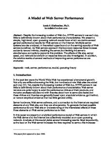
2. HTTP/1.1 Protocol Overview In this section we give a brief overview of the HTTP/1.1 data exchanges and discuss the factors that have a large impact on the end user response time. Though there are many types of web browsers and web servers, almost all of them support HTTP/1.1. The main functions of its specifications are persistent connections and pipelining. Persistent connections have a number of advantages: by opening and closing fewer TCP connections, CPU time is saved in routers and hosts (clients, servers, proxies, or gateways), and memory used for TCP control blocks can be saved in hosts, and latency on subsequent requests is reduced because no time is spent on a TCP connection’s opening handshake. Pipelining allows a browser to make multiple requests without waiting for each response, allowing a single TCP connection to be used much more efficiently, with much lower elapsed time. We investigated the HTTP/1.1 data exchanges between some web browsers and web servers, and found that the browser implements only multiple persistent TCP connections instead of pipelining. Though the maximum number of such multiple TCP connections differs from browser to browser, the basic data exchanges are as shown in Figure 1. This example shows the case where two persistent TCP connections are used.
In this paper, we focus on accurate simulation of the end user response time. This is one of the most important performance metrics for IT systems evaluation. We propose a web server performance modeling method and a parameter setting method that complement the “Tune protocols and parameters’’ section of SMARTE. The modeling method adapts service-time calculations in a gna_clsvr_mgr.pr.m depending on whether the contents are static objects (text, gif, or jpg) or dynamic objects (asp, cgi, etc.). We also describe a method that models a web server’s basic performance when one request is processed at the server and its multi-tasking performance when multiple requests are processed concurrently at the server. In addition, we mention how to set these parameters based on stress tests on an actual server, taking into account HTTP/1.1[3] behavior (e.g., multiple
It also shows that the HTTP response time experienced by the end user comes from the sum of three types of delay: network delay in each direction, service time at the client, and service time at the server. Though we can use OPNET to simulate basic HTTP/1.1 data exchanges and these service times, it is difficult to set up all the node performance parameters for accurate simulation. So we discuss methods for modeling web server performance and setting its parameters.
1
Network delay for downloading
PS[bytes/s] be the processing speed at the application layer, and OH[s] be the remaining service overhead, which does not depend on the content size. We consider ST1 for the static content as STstatic and ST1 for dynamically generated content as STdynamic. They are computed as follows.
Web server SYN SYN+ACK ACK HTTP: Get ∼.html
Network delay for uploading
SYN SYN+ACK ACK HTTP: Get ∼.jpg HTTP: Get ∼.gif
STstatic = HTTP: Get ∼.exe HTTP: Get ∼.mov
ST1
…
End user response time
Web browser
FS static PS
STdynamic = OH +
HTTP: Get ∼.gif
FIN ACK FIN ACK
FS dynamic
(3)
PS
Equations (2) and (3) are models that represent ST1 at the web server when the corresponding types of contents are required. The reason only STdynamic has the OH is that the OH for STstatic is considered to be much smaller than OH for STdynamic. Therefore, if we try to take into account the OH for STstatic, it is difficult for us to estimate its value. We implemented these calculations for the default simple server model in OPNET by modifying the gna_clsvr_mgr.pr.c.
Client service time Server service time
Figure 1: Overview of HTTP/1.1 protocol. 3. Web Server Performance Model In OPNET, though we can use a “detailed server model” to examine the performance of its interactions, there are situations where we really do not need detailed models for all servers or do not have performance information for all of them. So in this paper, we propose a web server performance modeling method using a simple server model that was slightly modified for easy parameter setting. Let ST1 be the basic performance, which is the average service time per request when one request is processed at the server, and let Loadn be the multi-tasking performance function, which degrades the basic performance of the server. Using this function, we can compute the average service time STn when n requests are concurrently processed at the server as the product of ST1 and Loadn. This equation is the same as the one for calculating the default simple server model in OPNET.
3-2. Setting the Parameters of ST1 The parameters of ST1 were calculated by analyzing data exchanges between an actual client and server. The data exchanges were measured at the client so as not to affect the web server performance. In addition, to remove the network delay between them, they were connected directly by a short cross cable. Let MST be the measured service time at the server. It can be obtained by analyzing the data exchanges, as shown in Figure 2.
Web browser
Web server
…
STn = ST1 × Load n
(2)
Server service time
(1)
Though Application Characterization Environment (ACE), an add-on module for OPNET, allows us to model an application’s behavior accurately, it does not help us to modify data exchanges that were imported from the application capture file. In contrast, our model described in the next section can cope with the situation where we want to customize the data exchanges. The next section shows how ST1 and Loadn can be modeled by a simple calculation instead of importing a capture file, and how to set up the performance parameters by analyzing the HTTP/1.1 data exchanges.
Server service time
Server service time Server service time
… Figure 2: Measuring the server service time.
3-1. ST1: Basic Performance Modeling A web server handles requests for a diverse collection of resources, ranging from static files to scripts that generate customized responses. It is considered that web requests can be categorized into two types, ones for: (1) static contents like html, jpg, and gif and (2) dynamically generated contents like ServerSide Include (SSI) and Common Gateway Interface (CGI). SSI instructs the web server to customize a static resource based on directives in an HTML-like file. CGI is invoked by the server as a separate process and dynamically generates an HTML file. Therefore, we propose adapting ST1 calculations according to the content type. Let FSstatic[bytes] be the size of static content, FSdynamic[bytes] be the size of dynamically generated content,
When we measure the MST, we need to take into account multiple persistent TCP connections. This illustration shows the case where the browser uses two persistent TCP connections concurrently to download the contents of a web page. We can obtain the “busy time” at the server from the diagram of “ACE AppDoctor statistics”. We regarded this “busy time” at the server as being equal to the sum of MSTs at the server, because it was almost the same as the result of manual summation. Strictly, however, it is not the same when multiple persistent TCP connections are used concurrently, because it is calculated for the closest request-response pair at the node. 2
as soon as possible after getting the page response, in order to keep the number of actively accessing users constant. By doing this, we measured RTn. Figure 3 shows the average response time per second for all the active users. Figure 4 shows the average response time of each virtual user, as the number of users increased from 1 to 48. From Figure 4, this can be approximated by a linear equation.
We also need each file size (FS) of the contents, which can be obtained from the measured trace file. Let p be the total number of contents and q be the number of dynamically generated contents. Then PS and OH can be calculated by solving the following equations.
∑ MST = ∑ OH i =0
i
j =0
∑ +
p
i =0
j
MSTk = OH k +
FSi
(4)
PS
FS k PS
( k = 0, K , q ) (5)
As an example, Table 1 shows the results for a certain web page, Webpage-A. This page had 18 content items including a dynamic one (p=18, q=1). The total file size for all contents was 54,007 bytes, and that of the dynamic content, FSdynamic, was 322 bytes. The sum of MST for all contents was 27.141 ms, and the MST for dynamic content, MSTdynamic, was 20.194 ms. Then PS and OH for this page were calculated using equations (4) and (5). PS was 7,727,796 bytes/s, and OH was 20.152 ms. These values are used in section 4 to validate the ST1 modeling. ST1 parameters p q p
i =0
FS i
∑
p
i =0
Webpage-A 18 1
322 bytes
MSTi
MSTdynamic PS OH
27.141 ms 20.194 ms 7,727,796 bytes/s 20.152 ms
Table 1: ST1 parameters.
STn RTn ≈ ST1 RT1
1 0.9 0.8 0.7 0.6 0.5 0.4 0.3 0.2 0.1 0
14:24
19:12
24:00
28:48
1.6
y = 0.0306x + 0.0075
1.4
2
R = 0.9995
1.2 1 0.8 0.6 0.4 0.2 0 0
3-3. Loadn: Multi-tasking Performance Modeling Here we consider how to set the multi-tasking performance function Loadn. It can be calculated as the ratio of STn to ST1 by equation (1). Let RT1 be the average response time when one request is processed at the server, and let RTn be the average response time when n requests are processed concurrently at the server. If there is no network delay, and the client service time and number of users are the same in both cases, then the ratio of STn to ST1 can be replaced by the ratio of RTn to RT1 as follows.
Load n =
9:36
Figure 3: Average response time per second.
54,007 bytes
FS dynamic
4:48
Elapsed time of stress test (min:sec)
Multi-tasking performance table
∑
1.6 1.4 1.2 1 0.8 0.6 0.4 0.2 0 0:00
Average response time (s)
q
Average response time per second (s)
p
10
20 30 Number of virtual users
40
50
Figure 4: Average response time and multi-tasking performance table. When we measured RTn, we paid attention to the following three points. First, as described above, we made some virtual users repeatedly access the target page to hit the server’s cache before measuring the data for RTn. If we had not done so, the requests when RT1 were measured would not have hit the cache while the requests when RTn were measured would have. Secondly, we set up the stress test so that each virtual user used only one TCP connection (that is, we did not use the multiple TCP connections described in section 2). This enabled us to make the number of virtual users the same as that of jobs processed concurrently at the server. Thirdly, we removed the delays caused by the network and the client from RTn. In general, the measured response time includes network delays and several client service times. Therefore, using equation (7), we estimated ExtraDelay, which denotes the sum of these delays and client service times. Table 2 shows the results for Webpage-A. (The reason the sum of MST was different from that in Table 1 is that the requests did not hit the cache in Table 1.) By using ExtraDelay, we can
(6)
3-4. Setting Loadn To measure the RTn, we used LoadRunner[4], a stress test tool that can emulate the behavior of a web browser in detail; we call this emulation a virtual user. Many virtual users can individually access the server. We set up 50 virtual users to repeatedly access Webpage-A to make the setting of Loadn easy. And three virtual users were set up to repeat their access during a period of only two minutes in order to hit the web server’s cache. The remaining virtual users were increased from one virtual user per 30 seconds up to 48 users. Each virtual user repeated its request 3
4-1. Validating ST1 Modeling Figure 5 shows the experimental environment for validating ST1 modeling. We set PS and OH as shown in Table 1. Since we do not need to model the contention at the CPU, we set the corresponding parameters as follows: the task contention mode was set to “contention already modeled” and the multi-tasking performance table was set to “no entries”. In the OPNET project for validation, modified client and server nodes were connected by a switching-hub using 100Base-T and the “switch packet switching speed” was set to 500,000 packets/s. The simulation was run for five minutes and the first minute of data was discarded to remove initial bias. As shown in Table 3, the measured response time was 38.912 ms, and the simulated average response time was 38.072 ms. If there had been a large difference in these response times, we could have handled it as a client overhead. Though we had prepared a new attribute “client overhead” in the client node, we did not need to set it in this example.
calculate Loadn as equation (8) and multi-tasking performance table as 1/Loadn. This is also shown in Figure 4.
ExtraDelay = RT1 − ∑i =o MSTi p
Load n =
RTn − ExtraDelay RT1 − ExtraDelay
(8)
47.727 ms
RT1
∑
(7)
P
i =0
MSTi
26.962 ms
ExtraDelay
20.765 ms
Table 2: Extra delay. 4. Validating the Proposed Methods In this section, we validate the ST1 and Loadn modeling and setting results. We used the OPNET Modeler V.8.0.C with PL16. The service time calculations at the gna_clsvr_mgr_service_time_compute() in the function block of gna_clsvr_mgr.pr.m were modified to implement this proposed modeling method. The important node parameters to match the stress test environment were as follows: In the diagram of “HTTP specification table”, “HTTP version” was set to “HTTP 1.1”; “max connections” and “number of pipelined requests” were set to “2” to model two concurrent multiple TCP connections; “request size (bytes)”, which means HTTP header size, was set to a constant 245 bytes from the average measured HTTP header size; and the other parameters were set to default values. The attributes of “TCP parameters” at the server and client nodes were set as “Windows 2000”. In the diagram of “IP processing information table” at the server, the “datagram forwarding rate” was set as 50,000 packets/s. Since the delay caused by IP processing was already modeled in PS at the application layer, the value was set to be large enough to avoid IP processing being a bottleneck in the server. In the diagram of “IP processing information table” at the client, the “datagram forwarding rate” was set to 8256.275 packets/s, which was calculated as 100 Mbps ÷ (1514 bytes * 8 bits).
Response time Measured Simulated
Webpage-A 38.912 ms 38.072 ms
Table 3: Response time. We then investigated the data exchanges by analyzing them using ACE. Figure 6 shows the measured and simulated data exchanges captured by the analyzer node in the simulation. Figure 7 shows the statistics analyzed by ACE AppDoctor. Since our prototype model was implemented so that STdynamic is calculated first, the simulated data exchanges look different from the measured ones. The number of “network packets” and the average “network packet bytes” were almost the same. And “busy time” at the server was also nearly the same. Therefore, ST1 was accurately simulated by the proposed ST1 modeling method and parameter setting method, confirming the effectiveness of these methods. Measured Measured data data exchanges exchanges
Stress test environment Client
Web Server
Win2000 Pro LoadRunner 7 Sniffer Pro
Win2000 Server IIS5
Short cross cable
Simulated Simulated data data exchanges exchanges
Simulation model Modified server node: -Adapt ST 1 calculations -Set the estimated PS, OH -Multi-tasking table: “ No
entry ”
For capturing data exchanges
Figure 6: Data exchanges.
Figure 5: Experimental environment for validating ST1 modeling.
4
Simulated Simulated statistics statistics
3.5 Average response time (s)
Measured Measured statistics statistics
Stress test Simulated -LoadnSimulated -default-
3 2.5 2 1.5 1 0.5 0 0
10
20
30
40
Request sending rate (requests/s)
Figure 7: AppDoctor statistics of Figure 6.
Figure 9: Validating Loadn.
4-2. Validating Loadn Modeling We performed many stress tests to validate Loadn. The scenario was that 50 virtual users individually repeated requests in a uniformly distributed time cycle after getting their own response. By changing the mean time cycle, we changed the rate of sending requests to the server. All stress tests were run for five minutes of elapsed time and the first minute of data was discarded to remove initial bias. This simulation had almost the same scenario as the previous one. The task contention mode was set to “simulate contention” and the multi-tasking performance table was set to the estimated 1/Loadn described in section 3-4. By changing the “page inter-arrival time”, we changed the rate of sending requests to the server during the simulation. Figure 8 shows the experimental environment for validating Loadn modeling. All simulations were run for five minutes, the first minute of data was discarded to remove initial bias, and the downlink utilization between the switch and the server was not a bottleneck—it was about 13%. We compared the average response time against the rate of sending requests to the server. For comparison, we also evaluated when the multitasking performance table was set to 1/X, which is the default in OPNET. The results are shown in Figure 9.
Stress test environment
In this figure, all the graphs are almost on the same curve up to the divergent point. The results using 1/Loadn were better than those using 1/X, and almost the same as the stress test results. This shows that Loadn was accurately simulated by these proposed modeling and parameter setting methods, confirming the effectiveness of these methods. If it is possible to measure RTn, we should use 1/Loadn as the multi-tasking performance table instead of 1/X. 5. Comparison with Using ACE In this section, we discuss the simulation results when we imported data exchanges using ACE. If we do not need to modify the data exchanges imported from the application capture file, ACE allows us to model an application’s behavior accurately as well as easily. We can use it as ST1 to drive OPET simulations, and thereby see how the application will behave in different network scenarios. We investigated how ACE can allow us to model STn. 5-1. Validating ST1 Modeled by ACE We investigated ST1 imported by ACE. The data exchanges were the same as those mentioned in section 4-1. The simulation environment was also set in almost the same way as for the simulations in section 4-1. Only the “datagram forwarding rate” at the client was changed to 50,000 packets/s, because the delay caused by IP processing was already modeled using data imported by ACE. Therefore, the value was set to be large enough—in the same way as for the server—to avoid IP processing being a bottleneck at the client. As shown in Table 4, the simulated average response time was 40.761 ms. That is not so different, so we can consider it as being almost the same as the measured one.
Simulation model
Short cross cable
Web Server Win2000 Server IIS5
Number of virtual users
Client Win2000 Pro LoadRunner 7
Modified server node:
0
Elapsed time of stress test
Response time Measured Simulated (ACE)
- Adapt ST1 calculations - Set the estimated PS, OH (when web server’s cache was hit) - Multi-tasking performance table: 1/X 1/Loadn ,
Webpage-A 38.912 ms 40.761 ms
Table 4: Response time compared with ACE.
Figure 8: Experimental environment for validating Loadn modeling.
We then re-investigated the simulated data exchanges by analyzing with ACE. Figure 10 shows the measured data exchanges that were shown in section 4-1 and data exchanges 5
captured by the analyzer node in the simulation. These data exchanges look almost the same. Figure 11 shows the statistics analyzed by ACE AppDoctor. The number of “network packets”, “network packet bytes”, and “busy time” at the server were also close to the same. This shows that ST1 modeled by ACE accurately modeled an application’s behavior and network data exchanges.
Average response time (s)
3.5
Measured Measured data data exchanges exchanges
Stress test Simulated -LoadnSimulated -defaultSimulated -Imported by using ACE-
3 2.5 2 1.5 1 0.5 0 0
10
20
30
40
Request sending rate (requests/s) Data Data exchanges exchanges simulated simulated by by using using ACE ACE file file
Figure 12: Comparison with using ACE. 6. Conclusion In this paper we presented a web server performance modeling method and its parameter setting method that complement the “Tune protocols and parameters” section of the SMARTE methodology. These methods are based on analyzing data exchanges between client and server and the results of various stress tests on an actual server. They allow us to simulate accurately the end user response time of web applications. Through some examples and comparison with using ACE, we demonstrated the effectiveness of these methods. These methods can also be applied to other servers providing other services such as FTP, email, and databases.
Figure 10: Data exchanges simulated by using ACE file.
Measured Measured statistics statistics
Statistics Statistics simulated simulated by by using using ACE ACE file file
If the multi-tasking performance table could be applied to the server performance when ST1 was imported by ACE, then ACE would be the best way to model STn. However, in the situation where we want to modify data exchanges, because ACE does not help us to modify them, our proposed methods are the best solution. Therefore, we plan to develop the node performance measurement module, which will make it easy to measure and set these complicated node parameters for accurate simulation of end user response time. References
Figure 11: AppDoctor statistics of Figure 8.
[1] Netcraft: Web server Survey (2002). http://www.netcraft.com/Survey /Reports/ .
5-2. Comparison with Using ACE in STn Modeling We investigated the STn modeling by using ACE. We imported the data exchanges that had hit the cache (as described in section 3-4) to the simulations as ST1. And we also set the multi-tasking performance table as the estimated 1/Loadn (described in section 3-4). Then, we simulated in almost the same way as in the simulations in section 4-2. Figure 12 shows the results. ACE was unable to model the performance degradation, but our model could. Therefore, our methods are useful for modeling STn at the server. These results confirm the effectiveness of our proposed methods.
[2] OPNET Technologies: “SMARTE with ACE”, “SMARTE without ACE”, Methodologies & Case Studies on OPNET Online Document. [3] R. Fielding, J. Gettys, J. Mogul, H. Frystyk, L. Masinter, P. Leach, T. Berners-Lee, “Hypertext Transfer Protocol –HTTP/1.1”, RFC2616 (1999). [4] Mercury Interactive, http://www.mercury.co.jp/ .
6