Weighting Techniques in Data Compression - Signal Processing ...

Weighting Techniques in Data Compression: Theory and Algorithms

PROEFONTWERP ter verkrijging van de graad van doctor aan de Technische Universiteit Eindhoven, op gezag van de Rector Magnificus, prof.dr. R.A. van Santen, voor een commissie aangewezen door het College voor Promoties in het openbaar te verdedigen op vrijdag 13 december 2002 om 16.00 uur

door

Paulus Adrianus Jozef Volf

geboren te Eindhoven

De documentatie van het proefontwerp is goedgekeurd door de promotoren:

prof.ir. M.P.J. Stevens en prof.dr.ir. J.P.M. Schalkwijk Copromotor: dr.ir. F.M.J. Willems

CIP-DATA LIBRARY TECHNISCHE UNIVERSITEIT EINDHOVEN Volf, Paulus A.J. Weigthing techniques in data compression : theory and algorithms / by Paulus A.J. Volf. – Eindhoven : Technische Universiteit Eindhoven, 2002. Proefontwerp. – ISBN 90-386-1980-4 NUR 965 Trefw.: datacompressie / informatietheorie / coderingstheorie. Subject headings: data compression / source coding / trees mathematics / information theory.

S UMMARY

T

thesis is concerned with text compression. Text compression is a technique used on computer systems to compress data, such that the data occupies less storage space, or can be transmitted in shorter time. The compressor has to compact the data in such a way that a decompressor can restore the compacted data to its original form, without any distortion. The algorithms discussed in this thesis process the data sequence symbol by symbol. The underlying idea of these algorithms is that the few symbols preceding the new symbol in the data sequence, called the context of that symbol, predict its probability distribution. Therefore, while processing the data sequence these algorithms collect statistics on how often a symbol follows a certain context, for different context lengths. These statistics are stored in a special data structure, the context tree. From the statistical information in the context tree the compression algorithms estimate the probability distribution of the new symbol in the data sequence for different context lengths. Since the estimates of the probability distribution for the different context lengths will differ, these estimates have to be combined into a single estimate. The main difference between the compression algorithms is in how they combine these different estimates. The project has been set-up around the context-tree weighting (CTW) algorithm, a recently developed data compression algorithm that efficiently weights over different context lengths. The goal is to position this algorithm as a viable solution in the data compression world, next to well-known algorithms like Lempel-Ziv and the PPM-family. Therefore, the final design should be a data compression program based on CTW, that proves its applicability on a regular PC. This leads to a set of requirements for its performance, its speed and its memory usage. The design process has led to two design proposals. The first proposed design consists of three components: an implementation of an arithmetic coder, a CTW implementation, and a forward decomposition. The arithmetic coder translates the estimated probability distributions for the data symbols into a code word. This design uses a straightforward implementation of the Witten-Neal-Cleary arithmetic coder. The CTW implementation is the modelling algorithm that estimates the probability distribution of the new symbol, based on its context, and on the data seen so far. This implementation is a refinement of a previous implementation. For the new implementation, both the computational work, and the data structures and search algorithms have been examined and redesigned. Furthermore, different pruning algorithms for the context trees have been investigated and evaluated. Finally, the parameters have been fine-tuned. The forward decomposition is a completely new component. It analyses the data in a first pass, and it converts the data symbols to bits by means of a decomposition, based on the Huffman code. The decomposition reduces the length of frequent symbols, while it tries to preserve the structure of HIS

iii

iv

S UMMARY

the original alphabet. This reduces the average number of updates of the context trees. The first complete design has been evaluated in terms of the requirements. It meets these requirements, but the performance requirement is only met in a “weak” way, i.e. only the average performance of the design, measured over a standard set of test files, is better than the performance of its competitors. The goal of the second proposed design is to improve the performance such that it is competitive on every individual file of the standard set of test files. A new idea is proposed to achieve this: let two different modelling algorithms process the data sequence in parallel, while for each symbol a third algorithm will try to switch to the modelling algorithm that performs locally best. This idea is implemented in the second proposed design by adding two components, the snake algorithm and the companion algorithm, to the first design. The companion algorithm is the second modelling algorithm, that runs in parallel to CTW. It is based on PPMA, and it has been specifically designed to be complementary to CTW. This algorithm has been simplified, without losing its desired modelling behaviour, and it has been modified, such that it can use the same data structures as CTW. The snake algorithm is a weighting technique that for every symbol combines the two estimated probability distributions that it receives from CTW and the companion algorithm. The snake algorithm is a derivative of the more complex switching algorithm. Both algorithms have been developed for this project. They are analysed and implemented here for the first time. The complete second proposed design has been evaluated. It meets the strict definition of the performance requirement, it is one of the best data compression programs to date, at the cost of a lower speed and a higher memory usage. By offering the user a choice between both design solutions, the project has been completed successfully. The most important contribution of this work is the idea of switching between two modelling algorithms. One way to improve a data compression algorithm is by trying to find efficient modelling techniques for different (often larger) classes of sources. This work presents an alternative. Switching proves to be an efficient method to design a system that benefits from the strengths of both modelling algorithms, without going through the effort to capture them into a single, more complex, modelling algorithm.

S AMENVATTING

H

onderwerp van dit proefschrift is tekstcompresssie. Tekstcompressie is een techniek die op computersystemen wordt toegepast om data te comprimeren, zodat de data minder plaats in beslag nemen, of zodat deze in kortere tijd verzonden kunnen worden. De compressor moet de data wel zodanig samenpakken dat een decompressor nog in staat is de samengepakte data weer in hun oorspronkelijke vorm te herstellen, zonder dat daarbij enige mate van vervorming optreedt. De compressie-algoritmes die in dit proefschrift besproken worden verwerken de datarij symbool voor symbool. De achterliggende gedachte bij deze algoritmes is dat het groepje symbolen dat aan het nieuwe symbool in de datarij voorafgaat, dit noemen we de context van het nieuwe symbool, zijn kansverdeling bepaalt. Daarom bouwen deze algoritmes tijdens het verwerken van de datarij statistieken op over hoe vaak een symbool op een bepaalde context volgt, en dit voor verschillende lengtes van de context. Deze statistieken worden opgeslagen in een speciale datastructuur, de context-boom. Aan de hand van de statistische informatie in de context-boom schatten de compressie-algoritmes de kansverdeling van het nieuwe symbool in de datarij, voor verschillende lengtes van de context. Aangezien de verschillende context-lengtes zullen resulteren in verschillende schattingen voor deze kansverdeling, moeten deze schattingen nog gecombineerd worden. De wijze waarop het compressie-algoritme de verschillende schattingen samenvoegt, verschilt per algoritme, en is een van de belangrijkste kenmerken van zo’n algoritme. Het project is opgezet rond het context-boom weeg (CTW) algoritme, een recent ontwikkeld datacompressie algoritme dat op een efficiënte manier over de verschillende context-lengtes weegt. Het doel is om aan te tonen dat dit algoritme net zo bruikbaar is in praktische toepassingen als bewezen algoritmes zoals Lempel-Ziv en de PPM-familie. Daarom moet het uiteindelijke ontwerp een datacompressieprogramma worden dat gebaseerd is op het CTW algoritme, en dat op een gewone PC uitgevoerd kan worden. Om dit te realiseren zijn er eisen aan het ontwerp gesteld op het gebied van de compressieratio, snelheid en geheugengebruik. Het ontwerpproces heeft uiteindelijk tot twee ontwerpvoorstellen geleid. Het eerste voorgestelde ontwerp bestaat uit drie componenten: een implementatie van een aritmetische coder, een CTW implementatie, en een voorwaartse decompositie. De aritmetische encoder vertaalt de geschatte kansverdeling van de datasymbolen in een codewoord. Het ontwerp gebruikt een eenvoudige implementatie van de Witten-Neal-Cleary aritmetische coder. Het CTW algoritme is het eigenlijke modelleringsalgoritme dat de kansverdeling van het nieuwe datasymbool schat, gebaseerd op zijn context en de datarij tot nu toe. De hier gebruikte implementatie is een verbetering van eerdere implementaties. Voor de nieuwe implementatie zijn zowel het rekenwerk, als ET

v

vi

S AMENVATTING

de datastructuren en de daarbij behorende zoekalgoritmes onderzocht en herontworpen. Bovendien zijn nog verschillende snoei-algoritmes voor de context-bomen onderzocht en geëvalueerd. Tenslotte zijn de optimale instellingen van de verschillende parameters vastgesteld. De voorwaartse decompositie is een compleet nieuwe component. Zij analyseert eerst de hele datarij, en bepaalt vervolgens een decompositie waarmee de datasymbolen in bits worden gesplitst. Deze decompositie is gebaseerd op de Huffman code en wordt zo geconstrueerd dat ze de lengte van veel voorkomende symbolen reduceert, terwijl zij de structuur van het originele alfabet probeert te behouden. Dit verkleint het gemiddeld aantal verversingen in de context-bomen. Het eerste volledige ontwerp is geëvalueerd om te bepalen in hoeverre er aan de gestelde eisen voldaan is. Het blijkt inderdaad aan de eisen te voldoen, maar de eis aan de compressieratio is slechts op een “zwakke” manier gehaald, dat wil zeggen, dat, gemeten over een bekende, vooraf vastgestelde, set van testfiles, alleen de gemiddelde compressie beter is dan die van concurrerende algoritmes. Het doel van het tweede voorgestelde ontwerp is de compressie zodanig te verbeteren dat het op elke afzonderlijke file van de set van testfiles, minstens vergelijkbaar presteert met de concurrentie. Om dit te bereiken is een nieuw idee voorgesteld: laat twee datacompressiealgoritmes parallel de datarij verwerken, terwijl een derde algoritme tussen elk datasymbool zal proberen over te schakelen naar het compressie-algoritme dat op dat moment, lokaal, het beste comprimeert. In het tweede ontwerp is deze opzet ge¨ımplementeerd door twee componenten, het snake-algoritme en het companion-algoritme, aan het eerste ontwerp toe te voegen. Het companion-algoritme is het tweede datacompressie-algoritme dat parallel zal werken aan CTW. Het is gebaseerd op PPMA, en het is speciaal ontworpen om zo complementair als mogelijk aan CTW te zijn. Dit algoritme is zoveel mogelijk vereenvoudigd, zonder dat het gewenste gedrag verloren is gegaan, en het is aangepast, zodanig dat dit nieuwe algoritme gebruik kan maken van de bestaande datastructuren voor CTW. Het snake-algoritme weegt de kansverdelingen die het voor elk symbool krijgt van zowel het CTW algoritme als het companion-algoritme. Het snake-algoritme is een afgeleide van het complexere switching-algoritme. Beide algoritmes zijn ontwikkeld voor dit project. Ze zijn hier voor het eerst geanalyseerd en ge¨ımplementeerd. Het volledige tweede ontwerpvoorstel is geëvalueerd. Het voldoet aan de strengste compressie-eis, het is een van de beste bestaande datacompressie-programma’s op dit moment, maar dit is ten koste gegaan van de compressiesnelheid en van het geheugengebruik. Door de gebruiker een keus te bieden tussen beide oplossingen, is het project succesvol afgerond. De belangrijkste bijdrage van dit werk is het idee om tussen twee parallel werkende modelleringsalgoritmes te schakelen. Een bekende manier om datacompressie-algoritmes te verbeteren is door te proberen steeds efficiëntere modelleringsalgoritmes te vinden, voor verschillende (vaak uitgebreidere) klassen van bronnen. Dit werk presenteert een alternatief. Het schakelen is een efficiënte methode om een systeem te ontwikkelen dat succesvol gebruik kan maken van de voordelen van twee modelleringsalgoritmes, zonder dat er veel inspanning moet worden verricht om beide algoritmes te vervangen door een enkel complex modelleringsalgoritme.

C ONTENTS Summary

iii

Samenvatting

v

1 Introduction 1.1 The context of the project . . . . . . . . . . . . . . . . . 1.2 Applications of data compression algorithms . . . . . . . 1.3 An overview of this thesis . . . . . . . . . . . . . . . . . 1.4 Some observations . . . . . . . . . . . . . . . . . . . . 1.5 The mathematical frame work . . . . . . . . . . . . . . 1.5.1 Sources . . . . . . . . . . . . . . . . . . . . . . 1.5.2 Source codes . . . . . . . . . . . . . . . . . . . 1.5.3 Properties of source codes . . . . . . . . . . . . 1.5.4 Universal source coding for memoryless sources 1.5.5 Arithmetic coding . . . . . . . . . . . . . . . . 1.5.6 The Krichevsky-Trofimov estimator . . . . . . . 1.5.7 Rissanen’s converse . . . . . . . . . . . . . . . 2 The design path 2.1 Original project description . . . . . . . . . . . . . . 2.2 Requirements specification . . . . . . . . . . . . . . 2.3 The design strategy . . . . . . . . . . . . . . . . . . 2.3.1 Step 1: The basic design . . . . . . . . . . . 2.3.2 Step 2: The forward decomposition . . . . . 2.3.3 Step 3: Switching . . . . . . . . . . . . . . . 2.4 Other investigated features and criteria . . . . . . . . 2.4.1 Parallel processing . . . . . . . . . . . . . . 2.4.2 Random access, searching and segmentation 2.4.3 Flexibility . . . . . . . . . . . . . . . . . . . 2.4.4 A hardware implementation . . . . . . . . . 2.5 The design process in retrospective . . . . . . . . . . vii

. . . . . . . . . . . .

. . . . . . . . . . . .

. . . . . . . . . . . .

. . . . . . . . . . . .

. . . . . . . . . . . .

. . . . . . . . . . . .

. . . . . . . . . . . .

. . . . . . . . . . . .

. . . . . . . . . . . .

. . . . . . . . . . . .

. . . . . . . . . . . .

. . . . . . . . . . . .

. . . . . . . . . . . .

. . . . . . . . . . . .

. . . . . . . . . . . .

. . . . . . . . . . . .

. . . . . . . . . . . .

. . . . . . . . . . . .

. . . . . . . . . . . .

. . . . . . . . . . . .

. . . . . . . . . . . .

. . . . . . . . . . . .

. . . . . . . . . . . .

. . . . . . . . . . . .

. . . . . . . . . . . .

. . . . . . . . . . . .

. . . . . . . . . . . .

1 1 2 4 5 6 6 7 9 11 12 14 16

. . . . . . . . . . . .

17 17 18 23 25 27 29 32 32 36 38 38 39

viii

CONTENTS

3 Subsystem 1: Arithmetic coder 3.1 Description . . . . . . . . . . . . . . . . . . . . . . 3.2 Basic algorithm . . . . . . . . . . . . . . . . . . . . 3.3 Algorithmic solutions for an initial problem . . . . . 3.3.1 Fundamental problem . . . . . . . . . . . . 3.3.2 Solution I: Rubin coder . . . . . . . . . . . . 3.3.3 Solution II: Witten-Neal-Cleary coder . . . . 3.4 Implementation . . . . . . . . . . . . . . . . . . . . 3.4.1 Changing the floating point representation . . 3.4.2 Implementing the Rubin coder . . . . . . . . 3.4.3 Implementing the Witten-Neal-Cleary coder . 3.5 First evaluation . . . . . . . . . . . . . . . . . . . .

. . . . . . . . . . .

4 Subsystem 2: The Context-Tree Weighting algorithm 4.1 Description . . . . . . . . . . . . . . . . . . . . . . . 4.2 Basic algorithm . . . . . . . . . . . . . . . . . . . . . 4.2.1 Tree sources . . . . . . . . . . . . . . . . . . 4.2.2 Known tree structure with unknown parameters 4.2.3 Weighting probability distributions . . . . . . 4.2.4 The CTW algorithm . . . . . . . . . . . . . . 4.2.5 The basic implementation . . . . . . . . . . . 4.3 Algorithmic solutions for the initial problems . . . . . 4.3.1 Binary decomposition . . . . . . . . . . . . . 4.3.2 A more general estimator . . . . . . . . . . . . 4.4 Implementation . . . . . . . . . . . . . . . . . . . . . 4.4.1 Computations . . . . . . . . . . . . . . . . . . 4.4.2 Searching: Dealing with a fixed memory . . . 4.4.3 Searching: Search technique and data structures 4.4.4 Searching: Implementation . . . . . . . . . . . 4.4.5 Searching: Performance . . . . . . . . . . . . 4.5 First evaluation . . . . . . . . . . . . . . . . . . . . . 4.5.1 The Calgary corpus . . . . . . . . . . . . . . . 4.5.2 Fixing the estimator . . . . . . . . . . . . . . 4.5.3 Fixing β . . . . . . . . . . . . . . . . . . . . . 4.5.4 Fixing the unique path pruning . . . . . . . . . 4.5.5 Evaluation of the design . . . . . . . . . . . . 5 Subsystem 3: The forward decomposition 5.1 Description . . . . . . . . . . . . . . . . . . . 5.2 Basic algorithm . . . . . . . . . . . . . . . . . 5.2.1 Investigating the forward decomposition 5.2.2 Computing the symbol depths . . . . . 5.2.3 Computing the symbol order . . . . . .

. . . . .

. . . . .

. . . . .

. . . . .

. . . . . . . . . . .

. . . . . . . . . . . . . . . . . . . . . .

. . . . .

. . . . . . . . . . .

. . . . . . . . . . . . . . . . . . . . . .

. . . . .

. . . . . . . . . . .

. . . . . . . . . . . . . . . . . . . . . .

. . . . .

. . . . . . . . . . .

. . . . . . . . . . . . . . . . . . . . . .

. . . . .

. . . . . . . . . . .

. . . . . . . . . . . . . . . . . . . . . .

. . . . .

. . . . . . . . . . .

. . . . . . . . . . . . . . . . . . . . . .

. . . . .

. . . . . . . . . . .

. . . . . . . . . . . . . . . . . . . . . .

. . . . .

. . . . . . . . . . .

. . . . . . . . . . . . . . . . . . . . . .

. . . . .

. . . . . . . . . . .

. . . . . . . . . . . . . . . . . . . . . .

. . . . .

. . . . . . . . . . .

. . . . . . . . . . . . . . . . . . . . . .

. . . . .

. . . . . . . . . . .

. . . . . . . . . . . . . . . . . . . . . .

. . . . .

. . . . . . . . . . .

. . . . . . . . . . . . . . . . . . . . . .

. . . . .

. . . . . . . . . . .

. . . . . . . . . . . . . . . . . . . . . .

. . . . .

. . . . . . . . . . .

41 41 42 42 42 43 45 48 48 49 49 50

. . . . . . . . . . . . . . . . . . . . . .

53 53 54 54 54 57 58 60 61 61 64 65 65 69 73 76 79 81 81 81 82 82 85

. . . . .

87 87 88 88 91 92

CONTENTS 5.3 5.4

ix

Implementation: Describing the forward decomposition . . . . . . . . . . . . . . 94 First evaluation . . . . . . . . . . . . . . . . . . . . . . . . . . . . . . . . . . . 96

6 Subsystem 4: The snake algorithm 6.1 Description . . . . . . . . . . . 6.2 Basic algorithm . . . . . . . . . 6.2.1 The switching method . 6.2.2 The switching algorithm 6.2.3 The snake algorithm . . 6.3 Implementation . . . . . . . . . 6.4 Improvements . . . . . . . . . . 6.5 First evaluation . . . . . . . . . 6.6 Discussion . . . . . . . . . . . . 6.6.1 Introduction . . . . . . . 6.6.2 An approximation . . . 6.6.3 The maximum distance . 6.6.4 The speed . . . . . . . . 6.6.5 A simulation . . . . . . 6.6.6 Conjecture . . . . . . .

. . . . . . . . . . . . . . .

99 99 100 100 101 103 105 107 108 109 109 109 110 111 111 112

. . . . . . . . . . . . . . . . .

115 115 116 116 117 118 120 120 120 121 123 124 126 126 126 127 128 129

8 Integration and evaluation 8.1 System integration . . . . . . . . . . . . . . . . . . . . . . . . . . . . . . . . . 8.1.1 The algorithmic perspective . . . . . . . . . . . . . . . . . . . . . . . . 8.1.2 The arithmetic perspective . . . . . . . . . . . . . . . . . . . . . . . . .

131 131 132 134

. . . . . . . . . . . . . . .

. . . . . . . . . . . . . . .

. . . . . . . . . . . . . . .

. . . . . . . . . . . . . . .

. . . . . . . . . . . . . . .

. . . . . . . . . . . . . . .

. . . . . . . . . . . . . . .

. . . . . . . . . . . . . . .

. . . . . . . . . . . . . . .

. . . . . . . . . . . . . . .

. . . . . . . . . . . . . . .

. . . . . . . . . . . . . . .

7 Subsystem 5: The companion algorithm 7.1 Description . . . . . . . . . . . . . . . . . . . . . . . 7.2 Basic algorithm . . . . . . . . . . . . . . . . . . . . . 7.2.1 Introduction . . . . . . . . . . . . . . . . . . . 7.2.2 The memoryless estimator for PPMA . . . . . 7.2.3 Combining the memoryless estimates in PPMA 7.3 Integrating PPMA in the final design . . . . . . . . . . 7.3.1 Restrictions for our PPMA implementation . . 7.3.2 Decomposing PPMA . . . . . . . . . . . . . . 7.3.3 Some implementation considerations . . . . . 7.3.4 Extending the range . . . . . . . . . . . . . . 7.4 Implementation . . . . . . . . . . . . . . . . . . . . . 7.5 Improvements . . . . . . . . . . . . . . . . . . . . . . 7.6 First evaluation . . . . . . . . . . . . . . . . . . . . . 7.6.1 The reference set-up . . . . . . . . . . . . . . 7.6.2 The set-up of the snake algorithm . . . . . . . 7.6.3 The set-up of the companion algorithm . . . . 7.6.4 Evaluation . . . . . . . . . . . . . . . . . . .

. . . . . . . . . . . . . . .

. . . . . . . . . . . . . . . . .

. . . . . . . . . . . . . . .

. . . . . . . . . . . . . . . . .

. . . . . . . . . . . . . . .

. . . . . . . . . . . . . . . . .

. . . . . . . . . . . . . . .

. . . . . . . . . . . . . . . . .

. . . . . . . . . . . . . . .

. . . . . . . . . . . . . . . . .

. . . . . . . . . . . . . . .

. . . . . . . . . . . . . . . . .

. . . . . . . . . . . . . . .

. . . . . . . . . . . . . . . . .

. . . . . . . . . . . . . . .

. . . . . . . . . . . . . . . . .

. . . . . . . . . . . . . . .

. . . . . . . . . . . . . . . . .

. . . . . . . . . . . . . . .

. . . . . . . . . . . . . . . . .

. . . . . . . . . . . . . . .

. . . . . . . . . . . . . . . . .

. . . . . . . . . . . . . . .

. . . . . . . . . . . . . . . . .

. . . . . . . . . . . . . . .

. . . . . . . . . . . . . . . . .

x

CONTENTS . . . . . . . . .

135 136 138 139 139 140 140 144 145

9 Conclusions and recommendations 9.1 Conclusions . . . . . . . . . . . . . . . . . . . . . . . . . . . . . . . . . . . . . 9.2 Innovations . . . . . . . . . . . . . . . . . . . . . . . . . . . . . . . . . . . . . 9.3 Recommendations . . . . . . . . . . . . . . . . . . . . . . . . . . . . . . . . . .

147 147 148 149

Acknowledgements

151

A Selecting, weighting and switching A.1 Introduction . . . . . . . . . . A.2 Selecting . . . . . . . . . . . A.3 Weighting . . . . . . . . . . . A.4 Switching . . . . . . . . . . . A.5 Discussion . . . . . . . . . . .

8.2

8.1.3 The data structure perspective . . . 8.1.4 The implementation perspective . . 8.1.5 Modularity . . . . . . . . . . . . . Evaluation . . . . . . . . . . . . . . . . . . 8.2.1 Our final design . . . . . . . . . . . 8.2.2 The competing algorithms . . . . . 8.2.3 The performance on the two corpora 8.2.4 The performance on large files . . . 8.2.5 The final assessment . . . . . . . .

. . . . . . . . .

. . . . . . . . .

. . . . . . . . .

. . . . . . . . .

. . . . . . . . .

. . . . . . . . .

. . . . . . . . .

. . . . . . . . .

. . . . . . . . .

. . . . . . . . .

. . . . . . . . .

. . . . . . . . .

. . . . . . . . .

. . . . . . . . .

. . . . . . . . .

. . . . . . . . .

. . . . . . . . .

. . . . . . . . .

. . . . . . . . .

. . . . .

. . . . .

. . . . .

. . . . .

. . . . .

. . . . .

. . . . .

. . . . .

. . . . .

. . . . .

. . . . .

. . . . .

. . . . .

. . . . .

. . . . .

. . . . .

. . . . .

. . . . .

. . . . .

. . . . .

153 153 153 154 155 156

B Other innovations B.1 The Context-Tree Maximizing algorithm . . . B.2 Extended model classes for CTW . . . . . . . B.3 The context-tree branch-weighting algorithm B.4 An incompressible sequence . . . . . . . . .

. . . .

. . . .

. . . .

. . . .

. . . .

. . . .

. . . .

. . . .

. . . .

. . . .

. . . .

. . . .

. . . .

. . . .

. . . .

. . . .

. . . .

. . . .

. . . .

159 159 160 162 163

. . . . .

. . . . .

. . . . .

. . . . .

. . . . .

. . . . .

. . . . .

References

165

Index

171

Curriculum vitae

175

1 I NTRODUCTION

1.1

T

T HE CONTEXT OF THE PROJECT

thesis describes the design and implementation of a text compression technique. Text compression – the term should not be taken too literally – is a small but very lively corner of the data compression world: it is the field of the universal lossless data compression techniques used to compress a type of data typically found on computer systems. Data compression techniques comprise all schemes that represent information in an other, more compact, form. This includes for example the Morse-code which represents the letters of the alphabet in sequences of dots, bars and spaces. One characteristic of data compression is that the compressed information cannot be used directly again: a decompression technique is required to restore the information in its original form. For example, in the old days, a telegraph operator would translate your telegram into a sequence of Morse-code symbols. These symbols are very convenient for the operator while transmitting the message over the telegraph wire, but they are more difficult to read than regular text. Therefore, the operator at the other end of the line would translate the received Morse-code symbols back into the original message. On computer systems all information, or data, is stored as sequences of zeros and ones, regardless of whether the data represents an English text, a complete movie, or anything in between. On such systems, a data compression program tries to compact the data in some special format, such that the data occupies less disk space or that it can be transmitted in less time. A decompression program restores the information again. Text compression requires that the combination of compression and decompression is lossless: the data after decompression should be identical to the data before compression. Lossless data compression is essential for all applications in which absolutely no distortion due to the compaction process is allowed. This is clearly necessary for source codes, executables, and texts, among others. But also for medical X-rays and audio recordings in professional studios, HIS

1

2

I NTRODUCTION

lossless compression is being used. Another type of data compression is lossy compression, where a small amount of distortion is allowed between the decompressed data and the original data. This type of compression is almost solely used for information dealing with human perception: the human eye and ear are not perfect, they are insensitive for some specific types of distortion. This can be exploited by allowing small distortions, which are invisible, or inaudible, in the decompressed data. This has the advantage that very high compression rates can be achieved. Examples are the JPEG standard for still picture compression (photos), and the MPEG standards for video and audio compression. MPEG compression is used on DVD-systems, and for broadcasting digital TV-signals. Finally, text compression techniques have to be universal. This means that they should be able to process all types of data found on computer systems. It is impossible for a text compression program to compress all possible computer files, but at least it should be able to compress a wide range of different types of files. This will be explored further in Section 1.4. In short, the goal of this project is to develop and implement a simple utility on a computer system that can compress and decompress a file. The design should achieve the best possible compression ratio, with the limited resources of a present-day PC. As a result, there are strict constraints on the memory usage and the compression speed of the design. One of the motivations of this project is the wish to show that the Context-Tree Weighting (CTW) algorithm [62], a relatively new data compression technique, is as useful in practical applications as some other, more mature algorithms, like Lempel-Ziv and PPM. Therefore, the text compression program should be based on the CTW algorithm. This is not a rigid restriction, since recently the CTW algorithm has already been used to achieve very high compression rates [48, 64].

1.2

A PPLICATIONS OF DATA COMPRESSION ALGORITHMS

Universal lossless data compression techniques have many applications. The two most straightforward applications are file compression utilities and archivers. Our final design will be a file compressor: a utility that uses a data compression technique to compress a single computer file. An archiver is a utility that can compress a set of computer files into one archive. File compressors and archivers are very similar, but an archiver also has to deal with various administrative tasks, e.g., store the exact name of the file, its date of creation, the date of its last modification, etc., and often it will also preserve the directory structure. In general an archiver will compress each file individually, but some archivers can cleverly combine similar files in order to achieve some extra compression performance. Both applications require a data compression technique that delivers a good compression performance, while they also need to be available on many different platforms. Well-known file compressors are GZIP and compress, well-known archivers are ZIP, ZOO, and ARJ. Universal lossless data compression techniques are also used by disk compressors, inside back-up devices and inside modems. In these three applications the data compression technique is transparent for the user. A disk compressor, e.g. Stacker, is a computer program that automatically compresses the data that is written to a disk, and decompresses it when it is being read from the disk. The main emphasis of such programs is the compression and decompression speed.

1.2 A PPLICATIONS

OF DATA COMPRESSION ALGORITHMS

3

Back-up devices, like tape-streamers, often use a data compression technique to “increase” the capacity of the back-up medium. These devices are mostly used to store unused data, or to make a back-up of the data on a computer system, just in case an incident happens. Therefore, the stored data will in general not be retrieved often, and as a result the compression speed is more important than the decompression speed, which allows asymmetrical data compression techniques. Also many communication devices, like modems, e.g. the V42bis modem standard, and facsimile-equipment, have a built-in data compression program that compresses the data just before transmission and decompresses it, immediately after reception. Compression and decompression have to be performed in real time, so speed is important. An interesting issue to consider is at which point in the communication link the data is going to be compressed. It is safe to assume that data compressed once, cannot be compressed again. If the user compresses the data (either on his system with a state-of-the-art archiver, or in the communication device), the resulting data is rather compact and the telephone company has to send all data to the destination. But if the user does not compress the data, the telephone company can compress the data instead, transmit fewer bits, while still charging the user the entire connection rate. Finally, lossless universal data compression techniques can be used as an integral part of databases. Simple databases will only contain text, but nowadays there are very extensive databases that contain texts in different languages, audio clips, pictures and video sequences. Data compression techniques can be used to greatly reduce the required storage space. But, the database software has to search through the data, steered by, sometimes very complex, queries, it has to retrieve a very small portion of the total amount of stored data, and finally it might have to store the modified data again. In order to be useful under such dynamic circumstances, the data compression technique will have to fulfil very strict criteria: at the very least it has to allow random access to the compressed data. At the moment such features can only be found in the most simple data compression techniques. An example of a complete database project with compression can be found in “Managing Gigabytes” [70]. The algorithms investigated and developed in this thesis for universal lossless data compression programs, can also be used in other applications. We illustrated this for our students with two demonstrations. The first demonstration is intended to show that compressed data is almost random. We trained a data compression algorithm by compressing several megabytes (MBytes) of English text. Next we let students enter a random sequence of zeros and ones, which we then decompressed. The resulting “text” resembled English remarkable well, occasionally even containing half sentences. The fact that compressed data is reasonably “random” is used in cryptographic applications, where the data is compressed before encrypting it. For the second demonstration we trained our data compression program on three Dutch texts from different authors. Then a student had to select a few sentences from a text from any of these three authors, and the data compression program had to decide who wrote this piece of text. It proved to have a success rate close to a 100 %, which was of course also due to the fact that the three authors had a completely different style of writing. This is a very simple form of data mining. The data compression algorithms investigated here compress the data, by trying to find some structure in the data. The algorithms can be altered such that they do not compress the data, but that they try to find the structure that describes the given data best, instead. In this way these algorithms search explicitly for rules and dependencies in the data.

4

1.3

I NTRODUCTION

A N OVERVIEW OF THIS THESIS

The structure of this thesis is as follows. Chapter 2 gives a complete overview of the design path followed towards the final design. First the original project description is discussed, followed by a very detailed requirements specification of the final design. Then the design process is described step by step from a high level of abstraction, linking the technical chapters, Chapters 3 to 7, together. This chapter also presents some initial investigations of possible extensions to the final design, that have been considered early in the design process, but that have not been included in the final design (e.g. parallel processing, and random access). Finally, in hindsight, the design process is reviewed and some points that could have been improved are indicated. Chapter 3 discusses in depth the implementation of an arithmetic coder for the final design. Based on the theory described in Chapter 1, two coders are investigated and evaluated on speed and performance. Chapter 4 discusses the CTW algorithm, starting from the theory up to its final implementation. It is shown that the CTW algorithm, a data compression algorithm for binary sequences, first has to be modified to handle non-binary sources. Next, the two basic actions of CTW, searching and computing, are investigated in depth. The resulting algorithms and data structures are implemented and evaluated. The forward decomposition, described in Chapter 5, is a new component. Four different decomposition strategies of the 256-ary source symbols are developed and some limitations are discussed. Finally, the implementations are evaluated. Chapter 6 and Chapter 7 form the main contribution of this work. A completely new system has been proposed, in which two data compression algorithms compress the source sequence simultaneously, while between source symbols a third algorithm switches to the algorithm that performs locally best. Chapter 6 describes the development, analysis and implementation of the snake algorithm, the algorithm that switches between the two data compression algorithms. Chapter 7 describes the development and implementation of the second data compression algorithm, that will run in parallel to CTW. This chapter also gives a preliminary evaluation of the complete design. Chapter 8 consists of two parts. In the first part the integration of the five components of the final design is discussed from four different views, relevant for this design. The second half gives an elaborate evaluation of the final design. Two set-ups of the design are proposed, and they are both compared in speed and performance to other state-of-the-art data compression algorithms. Chapter 9 concludes this thesis. It also lists the most important innovations in the final design, and it gives some recommendations for further research. To fully understand the workings of most modern data compression algorithms, like the Context-Tree Weighting (CTW) algorithm [62], some knowledge of the underlying mathematical theory is necessary. The remainder of this chapter will briefly introduce some of the most important information theoretical concepts. But before we start this mathematical introduction, the next section will look at data compression from a more abstract point of view: what is possible, and what isn’t?

1.4 S OME

1.4

OBSERVATIONS

5

S OME OBSERVATIONS

From an abstract point of view, text compression is nothing more than a simple mapping. Suppose that the original sequence, the source sequence, has length N, then a text compression program maps all binary source sequences of length N to (hopefully shorter) binary sequences, the code words. Here, we will assume that the code words form a, so-called, prefix code: each possible source sequence gets a unique code word, and a code word may not be identical to the first part (the prefix) of any other code word. In Section 1.5.2 we will show that these prefix codes are just as powerful as any other code. The first observation is that the compression of some sequences inevitably results in the expansion of other sequences. For example, take all binary sequences of length 4. Suppose that all 16 possible combinations can actually occur. For some reason we decide to compress sequence 0000 into 3 bits, and give it code word 000. Since we use 000 as a code word, we cannot use code words 0000 and 0001, therefore only 14 possible code words of length 4 (0010 to 1111) remain. We now have 15 code words in total, one short of the 16 code words we need. This can only be solved by extending one of the other code words at the same time. Suppose we extend code word 1111 to 5 bits, then we get two new code words (11110 and 11111), and we have 16 code words again: 1 of 3 bits, 13 of 4 bits and 2 of 5 bits. Note that the number of sequences that we want to compress is related to the length of their code words. You cannot compress a large fraction of all possible sequences to very short code words, because the number of available short code words will run out. This concept is formalized by the Kraft-inequality (see Theorem 1.1 in Section 1.5.2). Thus a good data compression technique has to be selective. A second observation is that one can achieve compression by replacing events that occur often by short code words. For example, consider the following sequence of 36 bits: 100011100110001011001011001000111010. It might not be directly clear how this sequence can be compressed. But a data compression technique that counts pairs of bits will find that the number of occurrences of these pairs is not uniformly distributed: 00 occurs five times, 01 once, 10 eight times and 11 four times. If it replaces these pairs by code words, such that the most common pair gets the shortest code word (e.g. 00 is mapped to 10, 01 to 110, 10 to 0, and 11 to 111), then it can successfully compress this sequence (in this case to 33 bits). 10 00 11 10 01 10 00 10 11 00 10 11 00 10 00 11 10 10 ↓ ↓ ↓ ↓ ↓ ↓ ↓ ↓ ↓ ↓ ↓ ↓ ↓ ↓ ↓ ↓ ↓ ↓ 0 10 111 0 110 0 10 0 111 10 0 111 10 0 10 111 0 0 Thus in this particular case, a data compression technique that counts pairs of symbols is successful in compressing the sequence. Actually, most data compression techniques use counting techniques to compress sequences. A third observation is that often the data compression technique cannot apply the counting technique directly. Therefore, many data compression techniques assume that all sequences they encounter have some common type of underlying structure such that they can count events that

6

I NTRODUCTION

are important for that class of structures. This is called modelling and it is the most complex topic in the field of data compression. In case the compression technique should only compress e.g. English texts, then English words and the English grammar rules form the underlying structure. Within this structure the compression technique could count e.g. word occurrences and sentence constructions. A last observation is that the data compression technique does not have to assume a structure that matches the structure in the sequence perfectly to be able to compress it. Our text compression program is universal, thus the data compression technique that we are going to use needs to be able to find the structure in many different types of sequences. Our technique will assume that the sequences obey a very basic structure: the probability of a source symbol is only determined by the (at most D) previous symbols in the sequence. This structure has the additional advantage that an implementation will require only simple counting mechanisms. Although many actual sequences will belong to much more complex classes of structures, often sequences from these classes will show the behaviour of the very basic structure too. So, by assuming a less specific structure, we trade in compression performance for universality and implementation complexity.

1.5

T HE MATHEMATICAL FRAME WORK

This section gives a concise introduction to some key ideas from information theory.

1.5.1

S OURCES

A source generates source symbols xn , with n = 1, 2, . . . , N, each from a source alphabet X . For now, we assume that the source alphabet is binary, thus X = {0, 1}. Xn is the random variable denoting the nth output of the source. A source sequence x1 , x2 , . . . , x N , also denoted by x1N , is generated by the source with actual probability Pa (x1N ) = Pr{X1N = x1N }. These probabilities satisfy Pa (x1N ) ≥ 0, for all x1N ∈ X N , and Pa (x1N ) = 1. x1N ∈X N

The actual probability Pa (x1N ) is a block probability over N source symbols. It is the product of the N actual conditional probabilities of the individual source symbols, as they are assigned by the source: N N Pa (x1 ) = Pa (xn |x1n−1 ). n=1

For the moment we will only consider memoryless sources. In that case the random variables X1 , X2 , . . . , X N are independent and identically distributed (i.i.d.) and consequently the N Pa (xn ). Biactual probability of a source sequence x1N can be computed with Pa (x1N ) = n=1 nary memoryless sources are defined by a single parameter θ, with θ = Pa (Xn = 1) for all n and 0 ≤ θ ≤ 1. Now, if a source sequence x1N generated by such a source contains t ones, then the block probability reduces to Pa (x1N |θ) = θ t (1 − θ) N−t .

1.5 T HE

1.5.2

7

MATHEMATICAL FRAME WORK

S OURCE CODES

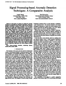
A binary source code is a function C that maps all possible binary source sequences x1N to binary code words of variable length1. A sequence x1N corresponds to code word c(x1N ) which has length l(x1N ). If the source sequence has length K · N, it can be split into K subsequences of length N. Each subsequence is then encoded individually with the source code, and the code words are concatenated. The decoder will be able to decode every possible series of code words back into their corresponding source sequence, if the source code is uniquely decodable. A source code is uniquely decodable if every possible series of code words could have been generated by only one, unique, source sequence [16]. Uniquely decodable source codes can have an undesirable property. It is possible that the decoder has to wait until the end of the series of code words, before it can start decoding the first code word. Therefore, we will restrict ourselves to a special class of source codes, called prefix codes, which do not have this property. In a prefix code, no code word is the prefix of any other code word. As a result, the decoder immediately recognizes a code word once it is completely received. The code words of a prefix code can be placed in a code tree, where each leaf corresponds to one code word. Such a code tree can be constructed because no code word is the prefix of any other code word. Example: Figure 1.1 shows two source codes for source sequences of length N = 2. Source code C1 is a uniquely decodable source code, but it is not a prefix code. After receiving 11 the decoder cannot decide between a concatenation of code words 1 and 1, and the first part of the code word 110 yet. Source code C2 is a prefix code with the same code word lengths. The code tree of this prefix code is shown on the right hand side. The decoder starts in the root node λ, and for every received symbol it takes the corresponding edge, until it reaches a leaf. As soon as it finds a leaf, the code word has been received completely, and can be decoded immediately.

x1N 00 01 10 11

C1

C2

1 110 010 00

0 100 101 11

1 λ

11

11

1 0

1

0

101

10

100

01

0 0

00

Figure 1.1: An example of a prefix code and its corresponding code tree. An important property of any uniquely decodable code, thus also any prefix code, is that the lengths of the code words should fulfil the Kraft-inequality. Theorem 1.1 (Kraft-inequality) The lengths of the code words of a prefix code fulfil the Kraft1

The source code described here is a so-called fixed-to-variable length source code. The arithmetic coder described in Section 1.5.5 is a variable-to-variable length source code. There exist also variable-to-fixed length source codes, but these are not used in this work.

8

I NTRODUCTION

inequality:

2−l(x1 ) ≤ 1, N

(1.1)

x1N

in which we sum over all source sequences x1N for which a code word c(x1N ) exists2 . The converse also holds. If a set of code word lengths fulfils the Kraft-inequality, then it is possible to construct a prefix code with these lengths. Proof: The proof is based on the relation between prefix codes and code trees. Take the longest code word length, lmax. A tree of depth lmax has 2lmax leaves. A code word c(x1N ) has a leaf at N depth l(x1N ) in the code tree, which eliminates 2lmax −l(x1 ) leaves at the maximum depth. Because the code words fulfil the prefix condition, two different code words will correspond to different leaves, and will eliminate disjoint sets of leaves at the maximum depth. Since all code words can be placed in one code tree, the sum of all eliminated leaves at maximum depth should not exceed the total number of available leaves. Therefore: N 2lmax −l(x1 ) ≤ 2lmax , x1N

which results in the Kraft-inequality after dividing by 2lmax . The converse also holds. Suppose a set of code word lengths fulfils the Kraft-inequality. Take a tree of depth lmax. Take the smallest code word length, say l, from the set and create a leaf in the tree at depth l, eliminating all of its descendants. Repeat this process for the smallest unused code word length, until all code word lengths have a corresponding leaf in the tree. The resulting tree is the code tree of a prefix code. This is a valid construction of a prefix code for three reasons. First, by constructing the shortest code words first and eliminating all their descendants in the tree, we guarantee that no code word is the prefix of any other code word. Secondly, let us denote the, say M, sorted code word lengths by l1 , l2 , . . . , l M , with l1 the smallest code word length and l M the largest. Suppose the first m code word lengths, with m < M, have already been placed in the tree. Then, m 2−li < 1, i=1

because the code word lengths fulfil the Kraft-inequality and there is at least one remaining code word length, lm+1. Thus there is still some remaining space in the tree. Thirdly, we have to show that this remaining space is distributed through the tree in such a way, that there is still a node at depth lm+1 available. The construction starts with the shortest code words, and the length of the first m code words is at most lm . A node at depth lm in the tree is then either eliminated by one of these first m code words, or it is unused and still has all of its descendants. Therefore, there is either no space left in the tree, or there is at least one unused node available at depth lm . Because 2

Note that for some sources not all source sequences can occur. These sequences have actual probability 0, and a source code does not have to assign a code word to these sequences. Strictly speaking, such sources need to be treated as a special case in some of the following formulas, e.g. by excluding them from the summations. This will unnecessarily complicate the formulas for an introductory section like this, therefore we decided to omit them here.

1.5 T HE


9

we already know from the second step that there is still space in the tree, and because lm+1 ≥ lm , the next code word can be constructed.¾ An important extension of the Kraft-inequality is given by McMillan. Theorem 1.2 (McMillan) The lengths of the code words of any uniquely decodable source code fulfil the Kraft-inequality. A proof of this theorem can be found in [16, section 5.5]. It states that the code word lengths of any uniquely decodable code must satisfy the Kraft-inequality. But a prefix code can be constructed for any set of code word lengths satisfying the Kraft-inequality. Thus by restricting ourselves to prefix codes, we can achieve the same code word lengths as with any other uniquely decodable code. Consequently, we pay no compression performance penalty by our restriction.

1.5.3

P ROPERTIES OF SOURCE CODES

The redundancy is a measure of the efficiency of a source code. The individual cumulative (over N symbols) redundancy of a code word c(x1N ) (with Pa (x1N ) > 0) is defined as: ρ(x1N ) = l(x1N ) − log2

1 , Pa (x1N )

(1.2)

in which the term − log2 Pa (x1N ) is called the ideal code word length of the sequence x1N (this name will be explained on page 10). The individual redundancy per source symbol is ρ(x1N )/N. The entropy H(X1N ) is the average ideal code word length:

H(X1N ) =

x1N ∈X N

Pa (x1N ) log2

1 , Pa (x1N )

(1.3)

in which we use the convention 0 log2 0 = 0. Now we can define the average cumulative redundancy ρ over all possible source sequences of a source code: 1 Pa (x1N )ρ(x1N ) = Pa (x1N )l(x1N ) − Pa (x1N ) log2 ρ = Pa (x1N ) x N ∈X N x N ∈X N x N ∈X N 1

= L−

1

H(X1N ).

1

(1.4)

An optimal prefix code minimizes the average cumulative redundancy ρ by minimizing the average code word length L, defined as L = x N ∈X N Pa (x1N ) · l(x1N ). The source coding theorem 1 gives bounds on the average code word length of the optimal prefix code. Theorem 1.3 (Source Coding Theorem) Consider a source with entropy H(X1N ) and a known actual probability distribution Pa (x1N ). Then the average length L of an optimal prefix code satisfies: H(X1N ) ≤ L < H(X1N ) + 1. (1.5) A prefix code achieves the entropy if and only if it assigns to each source sequence x1N a code word c(x1N ) with length l(x1N ) = − log2 Pa (x1N ).

10

I NTRODUCTION

Proof: First we prove the right hand side of (1.5). Suppose a prefix code assigns a code word with length l(x1N ) = log2 Pa (x1 N ) to source sequence x1N . These lengths fulfil the Kraft-inequality,

1

2−l(x1 ) = N

x1N ∈X N

2−− log2 Pa (x1 ) ≤ N

x1N ∈X N

2log2 Pa (x1 ) = 1, N

x1N ∈X N

thus it is possible to construct a prefix code with these lengths (this code is called the Shannon code, see [37]). The individual redundancy of this prefix code for a sequence x1N is upper bounded by, 1 1 1 ρ(x1N ) = l(x1N ) − log2 = log2 − log2 < 1, N N Pa (x1 ) Pa (x1 ) Pa (x1N ) and thus the average redundancy also satisfies ρ < 1. Substituting this in (1.4) results in the right hand side of (1.5). Since the optimal prefix code will not perform worse than this prefix code, it achieves the right hand side of (1.5) too. We prove the left hand side of (1.5), by proving that ρ ≥ 0. ρ=

Pa (x1N )l(x1N ) −

x1N ∈X N

=−

Pa (x1N ) log2

x1N ∈X N

1 Pa (x1N )

2−l(x1 ) Pa (x1N ) N

Pa (x1N ) log2

x1N ∈X N

N −1 2−l(x1 ) N = Pa (x1 ) ln ln 2 N N Pa (x1N ) x 1 ∈X N (a) −1 2−l(x1 ) N −1 ≥ Pa (x1 ) ln 2 x N ∈X N Pa (x1N ) 1  −1  N 2−l(x1 ) − Pa (x1N ) = ln 2 N N N N

x 1 ∈X

(b)

≥

−1 (1 − 1) = 0, ln 2

x 1 ∈X

(1.6)

where inequality (a) follows from the basic inequality ln a ≤ a − 1 and (b) from the Kraftinequality (1.1). Furthermore, we use the convention 0 log2 0 = 0. An optimal prefix code has a redundancy of 0, thus it has to fulfil inequalities (a) and (b) N with equality. For inequality (a) this is true only if 2−l(x1 ) / Pa (x1N ) = 1, and thus if l(x1N ) = − log2 Pa (x1N ). Furthermore, with these code word lengths inequality (b) will be satisfied with equality too.¾ The source coding theorem makes three important statements. First, the optimal prefix code has to chose the code word lengths as l(x1N ) = log2 Pa (x1 N ) , which also explains its name “ideal 1 code word length”. Secondly, as a direct consequence, the entropy is a fundamental lower bound on the average code word length of a prefix code. Thirdly, even though the ideal code word

1.5 T HE


11

length does not have to be an integer value, it is possible to design a prefix code that performs within one bit of the entropy.

1.5.4

U NIVERSAL SOURCE CODING FOR MEMORYLESS SOURCES

If the parameter of the memoryless source that generated the source sequence is known, then the actual probability distribution Pa (.) can be used in combination with the Shannon code to achieve a redundancy of less than 1 bit per sequence. Thus theoretically, for memoryless sources with a known parameter the coding problem is solved. Universal source coding deals with the situation in which this parameter, and consequently the actual probability distribution, are unknown. There are different types of universal source coding algorithms. This thesis follows the approach of Rissanen and Langdon [34]. They propose to strictly separate the universal source coding process into a modelling algorithm and an encoding algorithm. The modelling algorithm computes a probability distribution over all source sequences: it estimates the actual probability distribution. This estimate will be used as the coding distribution Pc (.) by the encoding algorithm. The encoding algorithm is a source code, e.g. the Shannon code, that uses this coding distribution Pc (.) to code the source sequence. For example, consider a universal source code for a binary memoryless source with unknown parameter. First, we need a good source code. The Shannon code cannot be used in practice, because it requires a table with all code words and the size of this table grows exponentially with the length of the source sequence. Section 1.5.5 discusses an arithmetic coder. This is a variable-to-variable length source code which is very computational and memory efficient, while it introduces only a very small coding redundancy of at most 2 bits. This source code operates sequentially, which means that it can process the source symbols one-by-one. In Section 1.5.6, the Krichevsky-Trofimov (KT) estimator is introduced. This estimator is a good modelling algorithm for binary memoryless sources. It also works sequentially, it estimates the probability distribution of the source symbols one-by-one. Thus, one possible universal source code for binary memoryless sources can be obtained by combining these two algorithms. Such a code will have the desirable property that it can process the source sequence sequentially: first the KT-estimator estimates the probability distribution of the next symbol in the source sequence and then the arithmetic coder codes this symbol. Note that the KT-estimator unavoidably introduces some additional redundancy. It does not know the parameter of the source that generated the source sequence, thus it has to estimate this parameter. Moreover, the decoder does not know this parameter either, so implicitly the KTestimator has to convey information about the parameter to the decoder. This results in some parameter redundancy. An upper bound on the parameter redundancy is computed in Section 1.5.6. Since the coding redundancy is at most 2 bits, independent of the length of the sequence, and since, as we will show later, parameter redundancy grows with the length of the sequence, the performance of universal source coding algorithms depends in general almost solely on the modelling algorithm.

12

1.5.5

I NTRODUCTION

A RITHMETIC CODING

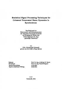
An arithmetic encoder (the idea is from Elias, see [21]) uses the conditional coding probabilities Pc (xn |x1n−1 ) of the individual source symbols to encode the source sequence. This requires both that the coding probabilities Pc (x1N ) of all source sequences should sum up to 1, and that the probabilities should satisfy Pc (x1n−1 ) = Pc (x1n−1 , Xn = 0) + Pc (x1n−1 , Xn = 1) for all n. One can partition the interval [0, 1) into disjoint subintervals, such that each possible sequence x1N has its own interval of size Pc (x1N ) (because of the first requirement mentioned above). Then, there exists a one-to-one relation between the sequence and its interval. We denote the lower boundary point of an interval by Q(.), thus the interval corresponding to sequence x1N is [Q(x1N ), Q(x1N ) + Pc (x1N )). Any point in this interval is sufficient to specify the entire interval, and thus to specify the source sequence. The idea is shown in Figure 1.2, for sequences of length 4. Suppose the source sequence is 1010, then the code word is the binary representation of a point in this interval, which is used by the decoder to retrieve the source sequence. Two issues remain to be explained: how to compute the interval corresponding to the source sequence efficiently, and how accurate does the point in this interval have to be described?

Pc (.)

Pc (.)

Pc (.) Pc (.)

Figure 1.2: The idea behind arithmetic encoding: coding a point in an interval. The subintervals are ordered according to the lexicographical order of the source sequences: a sequence x˜1n < x1n if for some index i, x˜i < xi , and x˜ j = x j for all j = 1, 2, . . . , i − 1. The lower boundary point is the sum of the probabilities of all sequences with a lower lexicographical order: Q(x1n ) = Pc ( x˜1n ). xñ1 0 and b > 0. With the Stirling bounds we can approximate the probability Pe (a, b). We get, √

a b a b 2 1 Pe (a, b) > √ 1 1 √ , (1.13) a+b πe 6 e 24 a + b a + b in which we also used (a − 12 )! = 2(2a)! 2a a! . Suppose the source has parameter θ, and the sequence has a zeros and b ones, then the actual probability Pa (x1N ) the source assigns to this sequence satisfies: a b

b a N a b Pa (x1 ) = (1 − θ) θ ≤ , a+b a+b since (1 − θ)a θ b achieves its maximum for θ = of a sequence x1N satisfies, ρ p (x1N )

b . a+b

Now, the individual parameter redundancy

1 1 (1 − θ)a θ b − log2 = log2 = log2 Pe (a, b) Pa (x1N ) Pe (a, b) √ 1+ 1 (a) 1 πe 6 24 (1 − θ)a θ b + log2 (a + b) + log2 a b ≤ log2 √ a b 2 2 a+b a+b (b)

0 or a > 0 and b = 0 we approximate the actual probability by Pa (x1N ) ≤ 1. Now we find, with the Stirling bounds (1.12), for Pe (0, N ), with N ≥ 2: (N − 12 )! (2N )! e− 12N 1 Pe (0, N ) = = 2N > √ √ . N! 2 N!N! π N 2

(1.15)

Now the individual redundancy of a sequence containing only ones (similar for only zeros) satisfies, (a) (b) 1 ρ p (x1N ) ≤ − log2 Pe (0, N ) ≤ log2 N + 1, (1.16) 2

16

I NTRODUCTION

in which (a) holds because Pa (x1N ) ≤ 1, and (b) holds for N = 1 since Pe (0, 1) = 12 , and for N ≥ 2, it follows from inequality (1.15). Combining (1.14) and (1.16) proves the theorem. ¾ Suppose that a sequence x1N generated by a memoryless source with unknown parameter has to be compressed. A universal source coding algorithm, consisting of the KT-estimator as the modelling algorithm, and the arithmetic coder as the encoding algorithm is used. Then the total redundancy, is upper bounded by: 1 ρ(x1N ) = l(x1N ) − log2 Pa (x1N )

1 1 1 N + l(x1 ) − log2 = log2 − log2 Pc (x1N ) Pa (x1N ) Pc (x1N )

1 1 1 (a) N − log2 = log2 + l(x1 ) − log2 Pe (x1N ) Pa (x1N ) Pc (x1N )

(b) 1 log2 N + 1 + 2. < 2 In (a) the estimated probability is used as coding probability and in (b) the bounds on the parameter redundancy (1.11) and the coding redundancy (1.4) are used. The parameter redundancy is introduced because the estimated probability, Pe (x1N ), is used as coding probability instead of the actual probability, Pa (x1N ).

1.5.7

R ISSANEN ’ S CONVERSE

The average cumulative parameter redundancy of the Krichevsky-Trofimov estimator is upper bounded by ρ p < 12 log2 N + 1. Rissanen [32] proved that this is the optimal result. He states that for any prefix code the measure of the subset A ⊂ [0, 1] of parameters θ (the measure is defined as A dθ) for which ρ < (1 − ) 12 log N tends to 0 as N → ∞ for any > 0. Thus the optimal behaviour of the redundancy for a memoryless source with unknown parameter is about ρ ≈ 12 log2 N, and consequently, the Krichevsky-Trofimov estimator performs roughly optimal. This concludes the general introduction to some necessary concepts from the information theory. More specific concepts will be addressed in following chapters.

2 T HE DESIGN

PATH

This chapter provides an overview of the design path followed towards the final design. It starts with the original project description, which is used to write the more detailed requirements specification. Next, the design process is described step by step in a global way, linking the technical chapters, Chapters 3 to 7, together. The last part of this chapter presents some initial investigations of possible extensions to the final design, that have been considered early in the design process, but that have not been included in the final design.

2.1

T

O RIGINAL PROJECT DESCRIPTION

original project description, prepared in 1996, specified the following goal and requirements. HE

Goal: design a data compression program, based on the CTW algorithm, that compresses English text files. The program has to fulfil the following requirements:

Its performance (expressed in bits/symbol) should be comparable to competitive algorithms available at the time of completion of this project. It should compress 10000 symbols per second on a HP 735 workstation. It may not use more than 32 MBytes of memory. It should be based on the context-tree weighting (CTW) algorithm. 17

18

T HE

DESIGN PATH

The program should work reliable: the decompressed data should be identical to the uncompressed data. The program may assume the following:

The text files will be at most 1 million ASCII symbols long. The core of this design will be the CTW algorithm [62]. Before the start of this new project the CTW algorithm has already been investigated intensively in the literature, and already two complete implementations of this algorithm existed. These two implementations were the starting point of our new design. The first implementation [48] achieves a performance, measured over a fixed set of files, that is comparable to the best competitive algorithms available at the start of our new project. But, this design is too slow and uses too much memory. The second implementation [65] has a slightly lower performance. But it is much faster and it uses considerably less memory. It actually already achieves the memory requirement set for our new design. At the start of this new project, we expected that a combination of the strengths of these two designs could result in an implementation that is close to the desired final design.

2.2

R EQUIREMENTS SPECIFICATION

The original project description does not describe the requirements of the final design in detail. Therefore, in this section we will investigate the different aspects of data compression programs, and we will immediately redefine the requirements of our data compression program. If necessary we make the first design decisions. First we will redefine the goal. Goal: design a data compression program, based on the CTW algorithm, that compresses data files on computer systems. We decided to extend the scope of our data compression program to all types of data commonly found on computer systems. Focusing on English texts alone limits the application of the new design too much. On the other hand, by increasing the number of different types of data sequences that should be processed, the performance of the final design on English texts will degrade. We will arrange the different aspects of data compression programs in five groups. First we have a necessary reliability requirement. Next, we have performance measures, which are aspects of the data compression program that can be measured. The third group, the algorithmic characteristics, are aspects of the program that are typical for the data compression algorithm that is used. The fourth group are the features. These are optional aspects of the program: if they are available, the user notices their presence and can take advantage of the additional functionality. Finally, there are implementation issues which only depend on the implementation of the algorithm, and in general the user will not notice these.

2.2 R EQUIREMENTS

SPECIFICATION

19

N ECESSARY REQUIREMENT: 1. It should work reliable.

P ERFORMANCE MEASURES : The performance measures are the only requirements that have been described in the original project description. But the description is rather global and needs to be specified in more detail. 2. Performance: The compression rate obtained by the program. Our requirement: Its performance should be competitive at the time of completion of the project. The performance of a data compression program is usually measured on a set of test files. These sets try to combine different types of files, such that they are representative of the type of files for which the program will be used. Two popular sets are the Calgary corpus [7] and the Canterbury corpus [5]. Here we will primarily use the Calgary corpus. The performance of our design will be compared to two state-of-the-art PPM-based algorithms (see [13]): the more theoretically based “state selection” algorithm [10], and the latest version of PPMZ, PPMZ-2 v0.7 [9]. Still, this requirement is ambiguous: should the performance be comparable on the entire corpus, or on every individual file? We will distinguish two performance requirements. The weak performance requirement demands that the performance of CTW on the entire Calgary corpus should be better than or the same as that of the best competitive algorithm. The strong performance requirement has two additional demands. First, because text files are specially mentioned in the original project description, CTW should compress each of the four text files in the Calgary corpus, , , , and , within 0.02 bits/symbol of the best competitive algorithm. This corresponds to a maximum loss of about 1 % on the compressed size, assuming that text is compressed to 2 bits/symbol. Furthermore, it should compress the other files within 0.04 bits/symbol of the best competitive algorithm. 3. Speed: The number of symbols compressed and decompressed per second. Note that for some data compression algorithms these speeds can differ significantly, but that is not the case for CTW. Discussion. In the original project description the measure speed is defined by a simple statement, while it actually is a complex notion. The speed that a certain implementation achieves depends on the algorithms that are implemented, the system on which it is executed, and the extent to which the code has been optimized for that system. A system is a combination of hardware and software. Important hardware elements are the CPU, the memory and the communication between these two. For the CPU, not only the clock frequency, but also the architecture is important. Some architectural properties are: the instruction set (RISC/CISC), the number of parallel pipe-lines (“super-scalar”), the number of stages per pipe-line,

20

T HE

DESIGN PATH

the number of parallel execution units, the width of the registers, the size of the primary instruction and data cache, the amount and speed of the secondary cache. The memory is also important, since our design will use around 32 MBytes of memory, too much to fit in the cache of a micro-processor. This means that the data structures have to be stored in the main memory and transfered to the cache when needed. Therefore, also the probability of a cache-miss, the reading and writing speed of the main memory and the width of the memory bus are determining the speed. Furthermore, the operating system also influences the compression speed. It can have other tasks running in the background simultaneously with the data compression program. In that case it has to switch continuously between tasks, which results in overhead, and most probably in repeatedly reloading the cache. Because compression speed depends so much on the system, a “system-independent” measure would solve the problem. One possibility is to count the average number of computations needed to compress a bit. Later, we will indeed count the number of operations to compare two sets of computations for the CTW algorithm, but such a measure is not general enough, since the computational work (additions, multiplications) accounts for only part of the total compression time. A significant other part of the compression time is used for memory accesses. It is impossible to make a general statement how the time required for one memory access compares to the time for one computation. Therefore, it is not possible to fairly compare two different implementations, if one implementation has more memory accesses than the other one, while it uses fewer computations. The focus of this thesis is directed towards finding good algorithms. We will use this machine, an HP 735, as a measurement instrument, to compare different algorithms. It is not intended to achieve the speed requirement by optimizing for this particular system, but only by improving the algorithms. It is possible that the source code of the final design will be made available to the public. In that case, optimizing for one machine is less useful. Therefore, we decided to keep the original, limited, speed requirement. The final design will be implemented in ANSI C. A standard available C-compiler will be used for compilation, and we will let it perform some system specific optimizations. In this way, we will not explicitly optimize for this single system, and our comparison are more representative for other systems. Note, that although we do not optimize our algorithms explicitly for this system, implicitly, but unavoidably, we do some system-dependent optimization. For example, during the design process some computations are replaced by table look-ups to improve the compression speed. Such a trade-off is clearly influenced by the hardware. The ideas for a parallel CTW implementation (Section 2.4.1) are an exception. These ideas are developed with a multi-processor system in mind. The goal was to split-up the CTW algorithm into parallel tasks, such that the communication between the different tasks is minimized. It needs a detailed mapping to translate these ideas to a single super-scalar or VLIW processor.

Our requirement: It should compress at least 10000 symbols per second on the available HP 9000 Series 700 Model 735/125 workstation. This workstation has a 125 MHz PA7150 processor. It achieves a SPECint95 of 4.04 (comparable to a 150 MHz PentiumI processor) and a SPECfp95 of 4.55 (slightly faster than a 200 MHz PentiumI processor).

2.2 R EQUIREMENTS

SPECIFICATION

21

4. Complexity: The amount of memory used while compressing or decompressing. The complexity can be specified for the encoder and decoder separately. Our requirement: The CTW algorithm has the same memory complexity for compressing and decompressing. In principle, the program should not use more than 32 MBytes of memory, but because both competitive state-of-the-art data compression programs use considerably more than 32 MBytes of memory, e.g. PPMZ-2 uses more than 100 MBytes on some files, it might be acceptable for our design too, to use more than 32 MBytes. 5. Universality: Data compression programs can be specifically designed for sequences with one type of underlying structure, e.g. English texts. Specializing can have advantages in performance, speed and complexity. But, if such a program is applied to sequences with a different underlying structure, then the performance can be poor. Thus, there is a trade-off between the universality of the program and the performance, complexity and speed of the program. Our requirement: It should be able to process all data files that can be encountered on computer systems. As mentioned, this is an extension on the original goal.

A LGORITHMIC CHARACTERISTICS : 6. Type of algorithm: What type of algorithm is used: a dictionary algorithm, or a statistical algorithm? Our requirement: It should be based on the CTW algorithm. 7. Type of encoding: Statistical algorithms need a separate coding algorithm. What type of coding algorithm will be used: e.g. enumerative coding, arithmetic coding, or one based on table look-up. Our requirement: Not specified. But implicitly it is assumed that an arithmetic coder will be used, since it appears to be the only viable solution at the moment. 8. Parallel computing: The ability of the program to spread the work load during compression, decompression, or both, over multiple processors. In some algorithms it is easier to allow parallel compression than to allow parallel decompression. So this feature could, for example, influence the balance of a certain program. Our requirement: Not specified. Support for parallel processing is very desirable, but not mandatory. 9. Balance: The difference between the compression speed and the decompression speed. In a balanced system the two speeds are comparable. Our requirement: Not explicitly specified, but the CTW algorithm is a balanced algorithm.

22

T HE

DESIGN PATH

10. Number of passes: The number of times the algorithm has to observe the complete data sequence before it has compressed that sequence. A sequential algorithm runs through the data sequence once, and compresses the symbols almost instantaneously. This is different from a one-pass algorithm, that might need to observe the entire data sequence before it starts compressing the sequence. Our requirement: Not specified. CTW is a sequential algorithm, and this is of course the most desirable form. 11. Buffering: The amount of delay the compressor or decompressor introduces while processing the data. This is closely related to the number of passes. Our requirement: Not specified. In sequential algorithms, buffering corresponds to the delay introduced by the algorithm between receiving an unprocessed symbol and transmitting it after processing. In one-pass or multi-pass systems such a definition is not useful. In that case, one might investigate how much of the source sequence needs to be buffered while processing the sequence. CTW is sequential and has a delay of only a few symbols. Preferably, the new design should introduce as little extra delay or buffering as possible.

F EATURES : 12a. Random Access: The ability of the decoder to decompress a part of the data, without the necessity to decompress all previous data. 12b. Searching: Is it possible to search for strings in the compressed data? 12c. Segmentation: The ability of the encoder to recognize different parts (segments) in the data, e.g. based on their underlying structure, and use a suitable algorithm for each segment. Our requirement: Support for random access, searching, or segmentation is very desirable, but not mandatory. The CTW algorithm in its current form does not allow any of these features.

I MPLEMENTATION ISSUES : 13. Compatibility: Is the program compatible across different platforms? Is it maybe compatible with other data compression programs? Our requirement: Not specified. Our final design should be compatible across different platforms: files compressed on one system should be decompressible on any other platform. In order to allow easy porting of the design, we will design the program as a set of ANSI C-files. Compatibility with other data compression algorithms is harder to achieve. This will be the first real CTW-oriented data compression program (the two older implementations are more intended for research purposes). Therefore, compatibility to other

2.3 T HE

DESIGN STRATEGY

23

programs can only be achieved by simply including their encoders and decoders. This is an unnecessary complication of our final design. 14. Modular design: Is the program completely integrated or is it designed as a collection of independent modules, which can be replaced by different modules, or which could be used in other designs? Our requirement: Not specified. The CTW algorithm already has, on a very basic level, a modular design. Partitioning the project in modules will not only ease the design process, but might also increase its use for future projects. 15. Flexibility: Is it possible to (efficiently) modify the program for special circumstances? Our requirement: Our new goal is to develop a universal data compression algorithm, thus it should be able to process any type of file. But it is of course possible to implement special facilities in the design for some specific types of data, e.g. pictures or texts. In principle we decided to implement a single universal data compression algorithm, without any special facilities, because otherwise a lot of time is invested to improve the performance of the final design for a small subset of files only. On the other hand, English texts are specifically mentioned in the original project description. A small research project has been conducted to include additional facilities for texts (see Section 2.4.3), but in the end it has not been used in the final design. As a compromise, we decided to define a stricter performance requirement for text files. 16. Scalability: Is it possible to scale the program? E.g., if we allow twice the memory will the program (or a slightly modified version) be able to use it efficiently, or not? Our requirement: Not specified. Every data compression algorithm has a maximum compression performance it can achieve given unlimited time and memory. Therefore, most data compression algorithms will perform better if they can use more processing power or more memory, but the increase in performance is in general not proportional to the increase in resources. The same holds for the CTW algorithm: more memory or more processing time will in general result in a (relatively small) increase in performance. Since, the speed and memory usage of our final design are restricted, we will not require a specific amount of scalability.

2.3

T HE DESIGN STRATEGY

Table 2.1 summarizes all design criteria of our design. The three key design criteria, performance, speed and complexity, have been our main concern while making most design decisions and therefore the following chapters will focus most on achieving these criteria. In addition to these criteria, five other criteria have been considered at some point during the design process. Table 2.1 refers for each of these criteria to the corresponding sections in this thesis. The remaining criteria were not considered during the actual design process. Three features, parallel

24

T HE

DESIGN PATH

Key design criteria: 2. Performance: Weak performance criterion: • at least as good on the entire Calgary corpus. Strong performance criterion: • at least as good on the entire Calgary corpus, • loss at most 0.02 bits/symbol on individual texts, • loss at most 0.04 bits/symbol on other files. 3. Speed: Compress 10000 symbols per second on a HP 735 work station. 4. Complexity: At most 32 MBytes. Other design criteria: 6. 10. 11. 13. 14.

Type of algorithm: CTW by specification. See Chapter 4. Number of passes: Preferable sequential. Discussed in Chapter 5. Buffering: As small as possible. Discussed in Sections 4.4.3, 7.3.4 and 8.1.3. Compatibility: Compatible across platforms. Discussed in Sections 4.4.1 and 8.1.2. Modularity: Desirable for future projects. Discussed in Section 8.1.5.

Investigated but rejected criteria (see Section 2.4): 8. Parallel compression or decompression. 12. Random access, searching and segmentation. 15. Flexibility. Not considered explicitly: 1. 7. 5. 9. 16.

Reliability: Essential property. Type of encoding: Not specified. Universality: Automatically fulfilled by design. Balance: Not specified. Scalability: Not required. Table 2.1: An overview of all design criteria.

2.3 T HE

25

DESIGN STRATEGY

compression and decompression, flexibility and random access, searching and segmentation have been investigated, but already in the beginning of the design process it was decided that these would not be implemented. Some of the work on the three criteria has been mentioned in Section 2.4. Finally, some criteria were trivial, impossible to achieve or not specified. These have not been mentioned explicitly in the remainder of this work. The remaining part of this section will follow the entire design process and it will show how the final design evolved.

2.3.1

S TEP 1: T HE BASIC DESIGN

Section 1.5.4 describes a universal source coding algorithm for memoryless sources. It consists of a modelling algorithm, the Krichevsky-Trofimov estimator, and a coding algorithm, an arithmetic coder. The final design has to use the CTW algorithm, which is a modelling algorithm for binary tree sources. The coding algorithm has not been specified, but at the moment the only viable choice is an arithmetic coder. A block diagram of a data compression program based on CTW has been shown in Figure 2.1. Here AE denotes Arithmetic Encoder, AD denotes Arithmetic Decoder, and c(x1N ) denotes the compressed data. The complexity of the CTW algorithm is much higher than the complexity of the arithmetic coder, thus it seems reasonable to focus on an efficient implementation for the CTW algorithm, without considering the interface with the arithmetic coder and then let the arithmetic coder solve possible communication problems. x1N Encoder

x1N Decoder

xn CTW

CTW

Pc (xn |x1n−1 )

Pc (xn |x1n−1 )

AE

xn

AD c(x1N )

Figure 2.1: The basic CTW compressor design.

T HE

BASIC DESIGN :

T HE

ARITHMETIC CODER

The principle of an arithmetic coder has been described in Section 1.5.5. The modelling algorithm, the CTW algorithm, estimates the probability distribution of the next source symbol, which is then used by the arithmetic coder to code this symbol. In our implementation the CTW

26

T HE

DESIGN PATH

algorithm estimates the probability distribution of single bits. These estimates use a fixed-point logarithmic representation: the logarithm of the probability is represented as an integer of which the lower bits denote the bits after the decimal point. Thus we have to design a binary arithmetic coder that can handle a probability distribution represented as logarithms. It has to fulfil the following requirements:

Performance: The optimal length of the code word for a source sequence with probability Pc (x1N ) is − log2 PC (x1N ) bits. In theory an arithmetic coder can be constructed that has a redundancy of less than two bits on the entire source sequence compared to the optimal length. This arithmetic coder requires computations of infinite accuracy, and cannot be used in practice. A practical arithmetic coder will have to round the probabilities, which will increase the redundancy. But a good arithmetic coder should be able to perform close to optimal. We require that our implementation of the arithmetic coder introduces a redundancy of less than 0.01 bit per source symbol of 8 bits. Complexity: An arithmetic coder uses a few registers, e.g., to store the probabilities and the lower boundary point of the interval. We require that our implementation uses a negligible amount of memory. Speed: The data compression program has to achieve a speed of 10 kBytes/second, or 80 kbits/second. Since the CTW algorithm is much more complex than the arithmetic coder, we will allocate only a small portion of the available time to the arithmetic coder. We require that the arithmetic coder may use at most 10 % of the available time, therefore it should achieve a compression speed of at least 800 kbits/second. Chapter 3 discusses the design of an arithmetic coder that fulfils these requirements. The final design is an implementation of the Witten-Neal-Cleary coder with 16 bits accuracy that accepts a binary probability distribution in a fixed-point logarithmic representation as input. This arithmetic coder has been assessed on three test sequences. Its redundancy is around 0.0001 bits/symbol, its compression speed is greater than 850 kbits/second and it uses only a few registers and a small table (just 3072 records of two bytes), so the memory requirements are negligible. Therefore this subsystem meets its goal and achieves all three requirements. T HE

BASIC DESIGN :

T HE CTW

ALGORITHM

The CTW algorithm should estimate the probability distribution of each source symbol. This estimate is then used in the arithmetic coder. Since the performance of the arithmetic coder is almost optimal, the performance of the entire data compression algorithm depends solely on the CTW algorithm. The algorithm has to fulfil the following requirements.

Performance: In combination with the arithmetic coder it should at least achieve the weak performance criterion, but preferably the strong performance criterion. Thus the performance of CTW should be at least as good as “state selection” and PPMZ-2 on the entire Calgary corpus. Preferably, it should also compress each of the four text files

2.3 T HE

DESIGN STRATEGY

27

within 0.02 bits/symbol of these two competitive algorithms, and each other file within 0.04 bits/symbol.

Complexity: The CTW algorithm should not use more than 32 MBytes of memory. Speed: The CTW algorithm, together with the arithmetic coder, should achieve a compression speed of at least 10 kBytes/second on our reference system. Chapter 4 discusses the design of the CTW algorithm. Our design uses a forward decomposition to decompose the source symbols. The context trees will be stored in a hash table of 32 MBytes. The records require only 6 bytes each, thus the hash table can contain almost 5.6 million records. Once the hash table is filled, the context trees will simply be frozen. The number of records that needs to be created is significantly reduced by a unique path pruning technique. In our implementation this technique requires a small additional buffer to store the most recent part of the source sequence. The computations are performed in a fixed-point logarithmic implementation and many computations are replaced by simple table-lookups. Finally, the performance has been improved by fine-tuning several variables, e.g. the estimator. This implementation of the CTW algorithm uses slightly more than 32 MBytes of memory, thus it meets the memory criterion (although for the hash table is too small). Its performance on the four text files is better than “state selection” and comparable to PPMZ2. But its performance on the other files of the Calgary corpus is worse by more than 0.04 bits/symbol, compared to PPMZ-2. Furthermore, it achieves a compression speed between 6 and 8 kBytes/sec. (6 kBytes/sec. on average on the Calgary corpus, 7 kBytes/sec. without ). Thus it does not meet the performance and speed criteria yet.

2.3.2

S TEP 2: T HE FORWARD DECOMPOSITION

The basic CTW algorithm estimates the probabilities of individual bits. It uses the straightforward ASCII decomposition (see Section 4.3.1) to translate source symbols into 8 bits, each bit has its own context tree, and consequently each symbol requires 8 estimations and thus 8 updates of the context trees. The number of updates is proportional to the memory usage and the computational complexity of the CTW algorithm. The average number of updates per symbol can be minimized by computing for each source sequence a special forward decomposition that minimizes the average number of bits per symbol. This will help the final design to meet the speed criterion. But it has two disadvantages. First, it requires an additional pass over the source sequence. Although sequential coding is not a crucial feature of our CTW implementation, we are reluctant to give it up, unless it results in a significant computational complexity reduction. Secondly, the encoder has to describe the forward decomposition for the decoder. More precisely, a special forward decomposition has to fulfil the following requirements.

Performance: The CTW algorithm with the special forward decomposition has to result in at least the same performance as the CTW algorithm with an ASCII decomposition, even though the special forward decomposition has to be described too.

28

T HE

DESIGN PATH

Speed: The forward decomposition should result in a significant increase in compression speed. At depth 10, and without (for which the hash table is too small), the current design achieves about 7 kBytes/sec., so the average speed should increase by about 40 % to meet the speed requirement. Complexity: The hash table is limited to 32 MBytes, therefore the memory criterion will be met. But at depth 10, requires about 8.3 million records, while the hash table can only hold 5.6 million records. To fully capture the entire model for , the number of records should decrease by about 30 %.

x1N

x1N xn = z1M

Encoder

z1M = xn

Forw. dec.

Forw. dec.

z1m−1

zm

Decoder

z1m−1 CTW

CTW Pc (zm |x1n−1 , z1m−1 )

Pc (zm |x1n−1 , z1m−1 ) AD

AE

zm

c(x1N ) Figure 2.2: The CTW design with a forward decomposition. The new design is shown in Figure 2.2. The encoder first computes the special forward decomposition. Then it translates each source symbol xn into a variable number of bits depending on the decomposition. Suppose symbol xn is described with M bits, z1 , z2 , . . . , z M 1 . The CTW algorithm receives the value of the next bit zm , and the values of the previous bits z1m−1 of this symbol, such that it knows which context tree it has to use to compress bit zm . The decoder first reads the special forward decomposition and then uses this decomposition to translate the individual bits back into the original source symbols. Chapter 5 discusses the design of a special forward decomposition. Our final design uses the decomposition called “Huf-IV”. The depths of the symbols in this decomposition are computed 1

Because the number of bits, and the values of the bits, depend on the value of xn , we should actually use a more elaborate notation: symbol xn is decomposed in some Mn bits, zn,1 , . . . , zn,Mn . But for sake of simplicity, we use the shorter notation in this thesis.

2.3 T HE

DESIGN STRATEGY

29

from the Huffman code for the source sequence, and the place of the symbols in the decomposition is obtained by a sorting technique that uses the initial values of the symbols. This special forward decomposition reduces the number of records by about 30 % (and by more than 40 % on ), it increases the compression speed by at least 25 % on most files, and almost doubles the average compression speed on the entire corpus to 11.9 kBytes/sec., while it also improves the compression performance by about 1 %. The CTW program with the Huf-IV forward decomposition uses slightly more than 32 MBytes of memory. It compresses the longer files of the Calgary corpus at about 10 kBytes/sec., and achieves an average speed of more than 10 kBytes/sec. It has a better performance on the four text files than PPMZ-2, and a slightly better average performance on the reduced Calgary corpus (the entire corpus except files and ). Therefore, this design meets the weak performance criterion plus all other key design criteria.

2.3.3

S TEP 3: S WITCHING

There is a new trend towards data compression programs that combine different compression algorithms. Because these algorithms have different characteristics, they will perform best on different types of files. By cleverly combining these algorithms, such programs are in general better equipped to achieve a good compression rate on a wide range of files. We investigated whether one of these new combining techniques can be used in our final design to improve its performance such that it will fulfil the strong performance criterion too, at the cost of only a small increase in memory and computational complexity. There are two basic techniques to combine different data compression algorithms in one program. First, the combining program can analyse the source sequence, and then decide which algorithm it will use to compress the entire sequence. Such a program can at best achieve global optimality: the compression rate on a source sequence can be as good as the best compression rate achieved by all algorithms it combines. Alternatively, the combining program could run different algorithms simultaneously, and use on each part of the source sequence the algorithm that performs locally best. Now it is possible that the combining program compresses a source sequence to a compression rate that is lower than that of each of the algorithms it combines. Because, the latter technique is more powerful, we decided to investigate one of its newest implementations, the switching method, here. It combines two data compression algorithms, therefore, such system requires two additional subsystems in our design: the snake algorithm and the companion algorithm. The snake algorithm is an efficient implementation of the switching method, and the companion algorithm is the second data compression algorithm that will run in parallel with CTW. Now, our design consists of five subsystems (Figure 2.3 shows the encoder; the decoder has to be extended similarly). S WITCHING : T HE

SNAKE ALGORITHM

Suppose the forward decomposition splits source symbol xn in M bits, z1 , . . . , z M . The snake algorithm receives for every bit zm , with m = 1, . . . , M, two estimates of the probability distribution, PA (zm |x1n−1 , z1m−1 ) from CTW and PB (zm |x1n−1 , z1m−1 ) from the companion algorithm. From

30

T HE

DESIGN PATH

x1N xn = z1M

Encoder

Forw. dec. zm

z1m−1 CTW

Comp. alg.

PA (zm |x1n−1 , z1m−1 )

PB (zm |x1n−1 , z1m−1 ) Snake alg. Pc (zm |x1n−1 , z1m−1 ) AE c(x1N )

Figure 2.3: The final design these two estimates, it computes the coding probability distribution Pc (zm |x1n−1 , z1m−1 ) of this bit for the arithmetic coder. The CTW algorithm already uses 32 MBytes of memory, and it achieves a compression speed of about 10 kBytes/second. In order to also achieve the strong performance criterion, we are willing to loosen the requirements on the memory complexity and the compression speed slightly. But it is a trade-off, in which the gain in performance has to be weighed against the increase in complexity. Therefore, it is very difficult to set strict constraints on the amount of time and memory that these additional subsystems may use and consequently, it is even more difficult to set such constraints for the snake algorithm alone.

Performance: The snake algorithm together with the companion algorithm, should improve the performance of CTW, such that the strong performance criterion is achieved. Therefore, for all files of the Calgary corpus it should perform within 0.04 bits/symbol of the best competitive algorithms, “state selection” and PPMZ-2. Complexity/Speed: The additional memory usage and the decrease in compression speed, due to the snake algorithm together with the companion algorithm, should be so small that the improvement in performance justifies their usage. This trade-off can only be evaluated after completion of this step of the design process.

2.3 T HE

DESIGN STRATEGY

31

Chapter 6 discusses the design of the snake algorithm. The snake algorithm weights both estimates for the probability distribution of the next symbol, such that the algorithm that performs locally best will dominate. The final design of the snake algorithm uses a fixed-point log representation for the floating point numbers. It uses almost no memory and it reduces the compression speed of the CTW algorithm by only 10 %. Thus the additional complexity caused by the snake algorithm alone seems reasonable. But because the snake algorithm is a greedy approximation of the switching algorithm we cannot guarantee that it is able to switch effectively between two data compression algorithms. This needs to be verified once the companion algorithm has been designed and implemented. S WITCHING : T HE

COMPANION ALGORITHM

The snake algorithm can achieve its highest gain if the two data compression algorithms between which it can switch have a complementary local performance. Because the CTW algorithm is fixed now, we should design a companion algorithm that is complementary to CTW. One of the weaker points of CTW is its performance on long repetitions and we decided to focus on this point. There are several algorithms, e.g. Lempel-Ziv type algorithms and PPM algorithms with a high maximum depth, that have a good performance on the long repetitive strings. Because it is easier to integrate PPM algorithms into our final design than Lempel-Ziv algorithms, we chose to use a PPM algorithm as our companion algorithm. The companion algorithm, together with the snake algorithm, has to fulfil the following requirements.

Performance: Together with the snake algorithm, it should improve the performance of the final design. The complete system should fulfil the strong performance criterion. Complexity/Speed: The additional memory usage and the decrease in compression speed, due to the companion algorithm together with the snake algorithm, should be so small that the improvement in performance justifies their usage. Chapter 7 discusses the design of the companion algorithm. Because the companion algorithm will only be used in parallel to CTW, its performance on a source sequence is not important, but only its ability to encode long repetitions efficiently matters. Consequently, we were able to both bias the companion algorithm even more in favour of long repetitions by increasing its maximum context length, and to greatly reduce the complexity of the algorithm. The final design implements PPMA. In order to reduce complexity, we modified it such that it uses only the already available information from the context trees for contexts of lengths up to and including D. Furthermore, to improve the performance, it has been extended to use much longer contexts and this extension requires an additional buffer of 2 MBytes. The combination of the snake algorithm and the companion algorithm improve the performance of CTW by more than 1 %, and it now meets the strong performance criterion. But, the complete system requires about 35 MBytes of memory, 10 % more than allowed, and more importantly, the compression speed is now reduced from 11.9 kBytes/sec. to only 6.6 kBytes/sec., far below the compression speed criterion.

32

T HE

DESIGN PATH

Still, the snake algorithm and the companion algorithm are a valuable addition to the data compression program. The computer technology has improved enormously since the start of the project. PPMZ-2 uses this additional computational power. It is slower than our entire final design, and it uses up to 100 MBytes of memory. Therefore, it seems best to implement the snake algorithm and PPM as a user option. Now the user can choose between a system, CTW alone, that achieves a very good performance, and meets all speed and memory requirements. Or the user can use the system with PPMA and the snake algorithm, which has a performance which is at least comparable to the best state-of-the-art programs, but which uses slightly more than 32 MBytes of memory, and which is about 34 % slower than the compression speed criterion. In the end, by offering users a choice between these two set-ups, we may conclude that we have completed the project successfully.

2.4

OTHER INVESTIGATED FEATURES AND CRITERIA

Three features or possible criteria of the final design have been investigated during the design process, but in the end it was decided not to implement these in the final design. In this section we will briefly describe some of the work and ideas concerning these features.

2.4.1

PARALLEL PROCESSING

There are two possible directions for allowing parallel processing in the CTW algorithm. We could either try to fit as much parallelism as possible into the CTW algorithm as it is at the moment. Or we could start with the assumption that we have multiple processors, and develop a CTW-like algorithm for this situation. This section describes two ideas for the first direction, and three for the second direction. In order to understand the limitations caused by the CTW algorithm, it is important to briefly describe the order of the computations in the estimation process. CTW collects its statistics in a context tree, which has a fixed maximum depth, say D. The context, the previous D symbols in the source sequence, specify one leaf of this tree. Coding, or more exactly the estimation, is done by estimating at each depth the probability of the new symbol, and then by weighting these estimates together. CTW starts at the highest depth, estimates the probability, updates the node, and continues with the parent node of this node. This process repeats itself until it reaches the root node which gives the final estimated probability distribution for the new source symbol. A node in a context tree can only be used for coding the next symbol if is has been updated for all previous symbols. This sets a fixed order in which a node has to be updated throughout the source sequence. As a result, this fixed order limits the maximum number of processors that can be used simultaneously. Without modifications, multiple processors can be effectively used in the encoder of the CTW algorithm. I The first technique introduces some sort of pipelining. As soon as a node has been updated for a certain source symbol it can (if necessary) be used to encode the next symbol. Thus

2.4 OTHER

INVESTIGATED FEATURES AND CRITERIA

33

while one processor is estimating the probabilities at depth 0 of the context tree for the current source symbol, a second processor could already estimate the probability at depth 1 of the context tree for the next symbol. Therefore, for a context tree of depth D, in total D + 1 processors could work simultaneously. II The second technique only applies to non-binary source symbols. As will be explained in Section 4.3.1 the CTW algorithm uses different context trees for coding each bit of a source symbol. Since the trees are updated independently, the updating, and thus the coding can be done concurrently. Both techniques are shown in Figure 2.4 for symbols consisting of 2 bits and context trees with maximum depth D = 2. Processors µ1 , µ3 , and µ5 can work simultaneously because they operate on nodes in the same context tree, but at different depths (technique I), and at the same time processors µ2 , µ4 , and µ6 can process the second bit (technique II). In total 6 processors ((D + 1) · M, in which M is the number of bits per source symbol) can work in parallel without any synchronization problems. Nodes from one of the two context trees for the second bit

Nodes from the context tree for the first bit

d=2 d=1 d=0

µ1

µ2

z1

z2 xn

µ3

µ4

z1

z2 xn+1

µ5

µ6

z1

z2 xn+2

Figure 2.4: Parallel encoding with the CTW algorithm. Techniques I and II cannot be used for the decoder. The first technique cannot be applied, because only after decoding the current symbol, the CTW algorithm can update the statistics in the context tree. But also the second technique cannot be applied because the CTW algorithm will use different context trees for the second bit of a symbol, depending on the value of the first bit. Since the decoder cannot look ahead in the source sequence like the encoder, it is very

34

T HE

DESIGN PATH

difficult to implement concurrent computing without modifying the CTW algorithm. Therefore, we investigated some ideas to redesign the CTW algorithm in order to simplify the parallel encoding and decoding. III The most straightforward idea is to split the source sequence in blocks and let each processor compress its own block, independently of the other blocks. This is shown on the left hand side of Figure 2.5 for two processors. Clearly, such a parallel CTW algorithm can be implemented easily. But this modification will have a huge impact on the performance. This is depicted in the stylized figure below the block diagram. It shows for each position in the source sequence the local compression rate achieved by the parallel CTW algorithm (the solid line) and by the regular CTW algorithm (the dotted line). The CTW algorithm is adaptive, so at the start of the source sequence the compression rate is poor, but it will rapidly converge towards its final compression rate. Since both blocks are compressed independently now, the parallel CTW algorithm has to adapt to the source sequence in both blocks: the “learning costs” are being paid twice. The difference between the solid line and the dotted line is the loss in performance. From a technical point of view, each block has its own set of context trees, therefore the statistics of the source sequence will be spread over more trees than before, and as a result the estimates will be less accurate. context trees

context trees

block II

block I

block II

local compression rate (bits/symbol)

local compression rate (bits/symbol)

block I

context trees

position in source sequence

order in which symbols are coded

Figure 2.5: Parallel coding with the CTW algorithm. IV An improved parallel CTW algorithm is depicted on the right hand side of Figure 2.5. It uses only one set of context trees. The context trees are “frozen”, as both processors code the next symbol in their block. Then, in one step, the context trees are updated for both source symbols. The advantage is clear, after every two source symbols the context trees are fully up-to-date. This is also visible in the stylized performance plot. In this plot the symbols are now ordered on the moment at which they are coded. In order to look at this parallel

2.4 OTHER


35

CTW algorithm from a different perspective, consider the sequential CTW algorithm that alternately encodes a symbol from both blocks. Such a sequential algorithm would achieve exactly the same performance as the regular sequential CTW algorithm, minus some small initialization losses for the second block. If this new sequential CTW algorithm is compared to the parallel CTW algorithm, then they behave identical, except that for the symbols in block II, the parallel CTW algorithm misses one update (the most recent symbol from block I). This results in a very small additional overall loss, which is indicated by the small area between the dotted line and the solid line in the performance plot in Figure 2.5. But this parallel CTW algorithm has an other disadvantage: the two processors will share at least one, but possibly more nodes, in the context trees. This might cause problems in the updating phase, because these nodes have to be updated for both symbols. This problem gets worse if more processors are being used. Then several nodes will have to be updated multiple times. Fortunately, most of these nodes will be in the lower parts of the context trees, and the coding of the new symbols will start in the upper part of the context trees. Therefore, one could collect all the multiple updates in a queue and use some dedicated processors to work through this backlog in updates, while simultaneously the other processors already start coding the new symbols. Such an algorithm would require additional administration in the nodes and additional communication between the different processors, so the gain in compression speed might not be proportional to the number of involved processors. V An elegant solution can be found by running the algorithms in the different blocks in a different phase. E.g., if the source symbols consist of two bits, then we can use two blocks. Assume that we decide to let the coding in block II run exactly one bit behind the coding in block I. Suppose, the CTW algorithm in block I should now code the second bit of, say, the eighth symbol. Then, the context tree for the first bit is fully updated for the eighth symbol in block I, and the CTW algorithm in block II can use it to code the first bit of its eighth symbol. In the next step, the CTW algorithm in block I can start with the first bit of its ninth symbol, with a context tree that now also includes the update of the first bit of the eighth symbol in block II. And, in block II, the CTW algorithm can compress the second bit of its eighth symbol, again, with a fully updated context tree. This technique has two advantages over technique IV. First, because the CTW algorithms in the different blocks process a different bit, they work in a different context tree, and their updates will never collide. Secondly, the context trees are always fully updated, thus the performance will be as good as the sequential CTW algorithm (except for some small initialization costs for the extra blocks). The drawback of this idea is that the source sequence can be split in at most the same number of blocks as the number of bits in each source symbol. Especially the fifth technique looks promising because it improves the speed of both the encoder and decoder, at a very low cost in performance. Still, we decided not to implement such a parallel CTW algorithm, because it is not an essential feature of our design, and the design time necessary to complete a parallel implementation had to be spent on achieving the key design criteria.

36

2.4.2

T HE

DESIGN PATH

R ANDOM ACCESS , SEARCHING AND SEGMENTATION

R ANDOM

ACCESS

Random access in the regular CTW algorithm is probably impossible. Therefore, we investigated different modifications in order to allow random access. Our investigations led us in two directions: either working from the bottom up, or looking from the top down. We started at the bottom by trying to develop a good random-access code for memoryless sequences. The performance of this code should be as close as possible to the performance of the Krichevsky-Trofimov estimator, which is used in the CTW algorithm to code memoryless sequences. This resulted in a random coding scheme [17, 67], which splits the source sequence into blocks, such that the decoder can decode one of these blocks without decoding the other ones. The scheme is based on enumerative coding. In enumerative encoding [14, 36] one first codes the parameter, followed by a description of the sequence given this parameter. Similarly, in our scheme the source sequence is coded in a series of parameter blocks and descriptive blocks. Each descriptive block corresponds to one block in the source sequence. The parameter blocks form a hierarchical structure, such that from a logarithmic number of parameter blocks the parameter for one descriptive block can be computed. One of the main challenges while developing this scheme was to be able to compute the starting points of the descriptive block and the parameter blocks in the compressed sequence without having to maintain a complete index. This scheme has a redundancy of only a fixed number of bits per block. Unfortunately, it was very difficult to implement this scheme in practice due to the very high accuracy required for the computations [17]. Therefore, this scheme is not a feasible “random access” substitute for the regular memoryless estimators yet. Alternatively, we started at the top by investigating the context-tree maximizing algorithm [50, 52, 53] (see also Appendix B). The maximizing algorithm finds the model that minimizes the description length, the MDL model. The description length of a source sequence is the length of the description of a model plus the length of the description of the source sequence, given that model. A compression program based on the maximizing algorithm is always a two-pass program. In the first pass it computes the MDL model for the source sequence and in the second pass it encodes the MDL model first, followed by the encoding of the source sequence itself. This algorithm could be more suitable for random-access than CTW, because it freezes the model and it separates the model description from the description of the source sequence (analogous to enumerative encoding). Suppose, we again want to split the source sequence into blocks, then we can encode the model description in various ways. We can e.g., describe the entire MDL model in advance, describe a separate MDL model for each block, or describe one core model (maybe even including some parameter information) that is used for every block, plus for each block a description of a refinement on this core model. Alternatively, we can order the blocks in some hierarchy, such that each block can be decoded after decoding at most a logarithmic number of other blocks. These schemes focus mostly on describing the model efficiently, but also the source sequence has to be described. The MDL model effectively splits the source sequence in memoryless subsequences, but the memoryless subsequences can have a variable number of symbols in each block of the source sequence. Therefore, this problem is similar to, but also more

2.4 OTHER


37

complex than the problem described in the previous paragraph, which we couldn’t satisfactory solve. Ultimately, one could decide to accept the losses and let the parameters adapt in each block individually. Unfortunately, experiments show that the performance of the maximizing algorithm is already considerably worse than the performance of the CTW algorithm and some of the improvements of the maximizing algorithm [52, 53] (e.g. on-the-fly, which mixes the model description and the description of the source sequence again) might not be possible in combination with random access. If random access causes a further degradation in performance, it might not be possible to achieve the performance criterion. In the end we decided not to implement these schemes. There is no comprehensive theory for random access. There are no known bounds on the minimum additional redundancy induced by random access and currently, everything beyond the most straightforward schemes still needs a lot of investigation before it can be applied in a practical design. S EARCHING Searching has not been investigated. If the compressed data has to be searched, without the availability of an index, then this problem is related to random access and, as we described above, we were not able to include random access in the final design. A compression program that allows random access and searching is described in [70]. It has been achieved by using a fixed code instead of an adaptive algorithm. S EGMENTATION There are several straightforward ways to implement segmentation. For example, an algorithm can analyse the data in detail, and choose for every segment the best data compression algorithm from a given set of algorithms, or the best set-up of one specific algorithm, like CTW. For the CTW algorithm, segmentation is important because CTW is a stationary algorithm. If the source is dynamic, and the parameters change significantly throughout the source sequence the performance of CTW might be poor. Therefore it would be useful to split the sequence in segments in which the source behaves more or less stationary. But it is very difficult to identify in the source sequence where one segment ends and a new one starts. The switching method (see Chapter 6) is a partial implementation of a segmentation strategy. It uses two data compression algorithms, the CTW algorithm and a Lempel-Ziv-like algorithm, that are running in parallel, and it allows a switch from one algorithm to the other one between any two source symbols. It is not an exact implementation of the segmentation behaviour, because both adaptive data compression algorithms observe the entire source sequence, thus also the segments on which the other algorithm is used. In a real segmentation implementation you might want to stop the adaptive algorithm that is currently not used. The final design uses an implementation of the switching method, thus segmentation has been achieved in the final design to some extent. Different approaches to segmentation, and running multiple data compression algorithms in parallel have been discussed in [69].

38

2.4.3

T HE

DESIGN PATH

F LEXIBILITY

Texts have been explicitly mentioned in the project description. Therefore, we investigated a possible extension of the CTW algorithms for texts. The CTW algorithm uses only the last, say 10, symbols of the source sequence to estimate the probability distribution of the next source symbol. But of course a text has a lot more structure, like e.g. grammar. Grammatical information can be added explicitly to a text by attaching a tag to each word. A tag could be a rather global specifier, like “noun”, “verb”, etc., or it could be more detailed, like “plural masculine noun”. These tags can be either added to the text by hand, or automatically with taggers. This last option leads to an interesting semi-two-pass strategy: in the “first pass” a tagger is used to label all the words, and possibly the punctuation, in the text, while in the second pass the text plus tags is being compressed. It has been reported that compressing a text with tags results in a shorter code word length than compressing the text alone [43, 44]. More in depth investigations on a CTW algorithm with tagged texts [6], shows more subtle differences. First of all, it is difficult to make a fair comparison, because compressing the tags induces additional complexity. Thus a Tag-CTW algorithm should be compared with a regular CTW algorithm with the same complexity, and consequently with a higher maximum context length. Also, because the TagCTW has more information, it will take longer before it converges to its best compression rate, therefore the algorithm should be compared on long texts (a few megabytes). From our initial investigations we concluded, that adding tags sometimes increases the performance slightly, say about 1 % on long texts, while in general it will not degrade the performance. Of course, the Tag-CTW could be further improved and optimized in order to gain more than 1 %, but still we decided not to use tags in our final design, because the gain is relatively small, and it would require that a complete tagger is added to the final design.

2.4.4

A HARDWARE IMPLEMENTATION

A hardware implementation of the CTW algorithm has not been mentioned in the project description. A hardware implementation is aimed at a different type of applications. While a software compression utility is cheap and can be used on existing computer systems, it will also be rather slow in general. Thus if an application requires a really high compression and decompression speed, then a hardware implementation could be useful. Hardware compression can be used inside communication equipment for computer networks (high speed modems, Ethernet cards, etc.), and inside storage equipment (tape streamers, hard disks), but also as an additional feature built into computer equipment, that can be used by any software package requiring the processing of huge quantities of data, like databases, or audio and video editing software. Before such a hardware implementation can be developed all properties of the device have to be investigated in detail. What format will the data be stored in? Should it be compatible to existing software or hardware solutions? Should one be able to randomly access the data? Should the data be protected against error-propagation? How fast should it be? After evaluating these criteria it might, for some purposes, be cheaper to use existing general purpose processors than to develop an application specific IC. All these considerations are beyond the scope of this thesis, but still we studied some possibilities for the CTW algorithm.

2.5 T HE

DESIGN PROCESS IN RETROSPECTIVE

39

Most existing hardware implementations of data compression algorithms are based on the Lempel-Ziv algorithms, e.g. the V42bis modem standard. The Lempel-Ziv algorithm processes the source sequence sequentially. The most straightforward hardware implementation of such an algorithm can use dedicated hardware to perform each step in the process sequentially, but very fast. The most time consuming step in a regular Lempel-Ziv implementation is the string matching step in the compressor. In this step a string, the next few symbols of the source sequence, is compared to a library consisting of a set of previously observed strings. This step can be implemented in parallel in hardware, which could result in a very significant gain in compression speed. There are various ways to implement this step in parallel in hardware, e.g. with a systolic array [40], or with associative arrays [8]. At the moment there has not been so much research on hardware implementations of adaptive algorithms, like CTW. The same considerations as for the dictionary based Lempel-Ziv algorithms apply. One could either design dedicated hardware to speed up the sequential operations, or one could try to redesign the algorithm in order to allow parallel processing in the hardware implementation. For this last option some of the parallel implementations of CTW as discussed before seem quite promising. Both the solution with processors working through the back-log in updates while the coding for the new source symbols has already started (technique IV), and especially the solution with the out-of-phase blocks (technique V), seem feasible in a hardware implementation. One step in the coding process of CTW has not been mentioned in the discussion of the parallel CTW implementation. Before a source symbol can be coded, first the correct path in the context tree has to be found. While of course an efficient searchable data structure can be applied, there are other options in a hardware implementation. For example, one can use associative memories. These memories consist of a decoder and the actual memory. Through the decoder these memories can not only be accessed based on their addresses, but also based on the contents of the memory cells. A key is provided to the memory decoder, and all memory cells that, according to some predefined relation, match that key, will offer their content serially on a data bus. One can imagine that, by offering a single key, in one operation all records on the context path are activated. In this way the speed can be increased even further. We didn’t study the design of a hardware implementation in detail, because a hardware design is not a part of our project description, but it is one of the angles from which we wanted to look at our design.

2.5

T HE DESIGN PROCESS IN RETROSPECTIVE

When the project started, two previous designs and their ideas were available. One design already achieved the weak performance criterion at that moment, but it used too much memory and compression time. The other design was faster and used less memory, it already met the memory criterion, but its performance was slightly worse. It was expected that a combination of the ideas used in these two designs would quickly result in a solid basis for our final design. Therefore, originally we intended to investigate the design of the data compression program from a broad perspective: e.g., random access, parallel processing, and maybe even some initial work on a hardware implementation.

40

T HE

DESIGN PATH

During the design process, we had to shift our focus more towards achieving the three key criteria. On one hand the performance of the competitive algorithms improved faster than expected, while on the other hand, it was more difficult to achieve the speed criterion than expected. This also explains our three step design process. After the first step, the design did not fulfil the performance criterion and the speed criterion. The objective of the second step was mainly to improve the compression speed, while the third step was aimed at improving the performance. In our design process the design was completed after each step and then evaluated. Only after the evaluation we could decide whether it was necessary to extend the design or not. The advantage of such a design process is that each step uses the completed design from the previous step as its basis and therefore the integration of the components will be simple. The disadvantage is that it is difficult to prepare for subsequent design steps, because only after evaluation of this design it will be clear which extension, if any, is necessary. As a result, design decisions are mostly made to improve the current design, but they could hamper following design steps. A prime example is the fixed data structure of the context trees, optimized for the CTW algorithm during the first design step, that later limits the choice of the escape mechanism for the companion algorithm in the third step (as discussed in Chapter 7). Furthermore, after completion of the project, it appears that some of the design decisions made early in the project might have to be reconsidered, with the knowledge that is available now. For example, in Chapter 4 we rejected the multi-alphabet CTW algorithm, because its computational complexity was to high. Later investigations [60] showed that some of the most complex steps can probably be greatly simplified. A multi-alphabet CTW could have greatly simplified the design of the snake algorithm and companion algorithm. But, such things are inevitable for long design processes in a rapidly changing field. Finally, we underestimated the great difficulties that still need to be overcome before additional features, like random access and parallel processing can be efficiently implemented. Most work on these features had to start from the very beginning, and although some progress has been made, it will still take a considerable amount of research before such ideas can be implemented in a practical design. During this project we have developed many innovative ideas. Some of these ideas have been used in the final design (the special forward decomposition, switching, and the decomposition of PPM, among others), but others were not well suited for our final design. Appendix B briefly describes some of the results obtained during this project that have not been used in our final design. Most of the new ideas have been published in papers. Ultimately, we realized an innovative design, split up in two programs, that meets its goal and achieves all key criteria. We believe that the project has been concluded successfully.

3 S UBSYSTEM 1: A RITHMETIC

CODER

This chapter discusses the implementation of the arithmetic coder for the final design. Based on the theory described in Chapter 1, two coders are investigated and evaluated on speed and performance. Both coders meet the design criteria, and in the end the Witten-Neal-Cleary coder is chosen because it has a marginally smaller redundancy.

3.1

D ESCRIPTION

T

HIS chapter is concerned with the design of an arithmetic coder. The arithmetic coder gets a binary probability distribution in a fixed-point log-representation from the CTW algorithm. The final implementation has to fulfil the following requirements:

The final design should achieve a code word length that is at most 0.01 bits/symbol longer than the optimal code word length of − log2 P(x1N ) bits, in which P(x1N ) is the coding probability of the source sequence1 . The final design should use only a negligible amount of memory. The final design should achieve a compression speed of at least 800 kbits/second. In this chapter two practical binary arithmetic coders will be described, the Rubin coder and the Witten-Neal-Cleary coder, and the resulting implementations will be tested on three test sequences to check whether they fulfil these criteria. 1

In this chapter we omitted the subscript and P(x1N ) denotes Pc (x1N )

41

42

S UBSYSTEM 1: A RITHMETIC

3.2

CODER

B ASIC ALGORITHM

The basic arithmetic coding algorithm, called the Elias algorithm (see [21]), has already been described in Section 1.5.5 for binary source symbols. The encoder is a direct implementation of the update rules and the length assignment. The following steps describe the binary encoder.

P(∅) = 1 Q(∅) = 0 xn n = 1, 2, . . . , N P(x1n ) = P(x1n−1 ) · P(Xn = xn |x1n−1 ) Q(x1n ) = Q(x1n−1 ) + P(x1n−1 ) · P(Xn < xn |x1n−1 )

c(x1N ) = Q(x1N ) · 2l(x ) · 2−l(x ) l(x N ) = − log2 P(x1N ) + 1 N

N

The Elias algorithm results in a code word length l(x1N ) which is at most two bits above the optimal length. The encoder uses only two floating point numbers ( P(.) and Q(.)), and at most one addition and two multiplications per source symbol. The decoder first determines a threshold value T (.). The threshold is the exact point at which the interval will be split in the next step. If the received code word c(x1N ) is below this threshold, then the next symbol is a ‘0’, otherwise it is a ‘1’.

P(∅) = 1 Q(∅) = 0 xn n = 1, 2, . . . , N T (x1n−1 ) = Q(x1n−1 , xn = 1) = Q(x1n−1 ) + P(x1n−1 ) · P(Xn = 0|x1n−1 ) c(x1N ) < T (x1n−1 ) xn = 0 xn = 1 P(x1n ) = P(x1n−1 ) · P(Xn = xn |x1n−1 ) Q(x1n ) = Q(x1n−1 ) + P(x1n−1 ) · P(Xn < xn |x1n−1 )

3.3 3.3.1

A LGORITHMIC SOLUTIONS FOR AN INITIAL PROBLEM F UNDAMENTAL PROBLEM

The Elias algorithm has a fundamental problem, which prevents it from being implemented as described in the previous section. It assumes that the computations are carried out with infinite accuracy and as a result, registers P(.), Q(.), and T (.) can become infinitely long. This problem has been solved in the latter part of the 1970s. In 1976 Pasco [30] described a rounding technique to fix the size of the register for P(.), but it still required an unbounded register for the lower boundary point. Also in 1976 Rissanen [31] published an arithmetic coder with fixed length registers, but this coder creates the code word from right to left, thus the encoding can only start after the entire source sequence is observed. In 1979 Rissanen and Langdon [33] mentioned that they had an arithmetic coder that uses only fixed length registers and that constructs the code

3.3 A LGORITHMIC

SOLUTIONS FOR AN INITIAL PROBLEM

43

word from left to right. They applied for a patent on this technique, which was granted in 1984 [23]. But, also in 1979 Rubin [35] published his practical implementation of an arithmetic coder with fixed length registers only. First the length of the register P(.) containing the interval size will be fixed. The size of the interval, the probability of the sequence so far, monotonically decreases. Thus the representation of the interval size will start with a growing number of zeros. Furthermore, the number of significant bits following these zeros can be fixed to, say, F bits by rounding after each operation at the cost of a small loss in performance. Now, a register of fixed-size F can be used to represent the size of the interval as follows. Before the new symbol is encoded, this register will be scaled until it uses its full accuracy by shifting out the leading zeros. In other words, this register containing the significant bits will be shifted to the right along the (infinitely long) register containing the lower boundary point. Next, the interval can be split into two subintervals, each subinterval size rounded to an accuracy of F bits. The new interval size will then still fit in the fixed size register. Even with a fixed-size register for the interval size, the representation of the lower boundary point still grows with the length of the sequence. Suppose the probability is indeed truncated to F significant bits. The new symbol will split this probability into two parts, and in case the new symbol is a ‘1’, the probability in case the symbol was a ‘0’ has to be added to the lower boundary point. Suppose we already scaled k times, and let us denote the representation of the lower boundary point by 0.q1 q2 . . . qk+F and the representation of the significant bits of the probability by p1 p2 . . . p F . Then the new lower boundary point is: 0. q1 q2 . . . qk qk+1 qk+2 . . . qk+F 0. 0 0 . . . 0 p1 p2 . . . p F + 0. q1 q2 . . . qk qk+1 qk+2 . . . qk+F . Now, it is clear that the first k bits of q1 q2 . . . qk cannot be transmitted yet, because a carry can occur, which can propagate through the entire register containing lower boundary point. Here, two solutions will be investigated that allow the first bits of Q(.) to be transmitted: the Rubin coder, which prevents a carry-over from happening altogether, and the Witten-Neal-Cleary coder, which uses an elegant carry blocking scheme.

3.3.2

S OLUTION I: RUBIN CODER

The Rubin algorithm [35] is an implementation of a binary arithmetic coder with two F bits registers, P R (.) and Q R (.). Register P R (.) is an integer representing the significant bits of P(.). The bits preceding the bits in this register are all zero. Register Q R (.) is an integer representing the F least significant bits of Q(.). The bits preceding the bits in this register should be fixed. Therefore, the registers have to fulfil the following property, for any n = 1, 2, . . . , N: 0 ≤ Q R (x1n ) < Q R (x1n ) + P R (x1n ) ≤ 2 F .

(3.1)

The second inequality holds because P R (.) is a positive integer. The last inequality guarantees that a carry-over will not occur.

44


CODER

The Rubin algorithm realizes bound (3.1) by scaling the two registers only if the first bit of the Q-register is fixed. There are two cases in which the first bit of the Q-register is fixed. First, if at some point Q R (x1n ) + P R (x1n ) ≤ 2 F−1, then the most significant bit of Q R (.) is fixed at a zero. Secondly, if at some point Q R (x1n ) ≥ 2 F−1, then the most significant bit of Q R (.) is fixed at a one. Thus, the Rubin algorithm will scale the registers until, Q R (x1n ) < 2 F−1 < Q R (x1n ) + P R (x1n ).

(3.2)

holds. As long as bound (3.2) is fulfilled, the most significant bit of Q R (.) can still take either value. The encoder is a straightforward implementation of the scaling rule. Before it divides the interval in two subintervals it scales the registers until bound (3.2) is satisfied.

P R (∅) = 2 F Q R (∅) = 0 n = 1, 2, . . . , N ! Q R (x1n−1 ) < 2 F−1 < Q R (x1n−1 ) + P R (x1n−1 ) " Q R (x1n−1 ) + P R (x1n−1 ) ≤ 2 F−1 # $ %& Q R (x1n−1 ) = Q R (x1n−1 ) · 2 P R (x1n−1 ) = P R (x1n−1 ) · 2 Q R (x1n−1 ) ≥ 2 F−1 # $ %& Q R (x1n−1 ) = (Q R (x1n−1 ) − 2 F−1 ) · 2 P R (x1n−1 ) = P R (x1n−1 ) · 2 (a)

P R (x1n ) = P(Xn = xn |x1n−1 ) · P R (x1n−1 ) Q R (x1n ) = Q R (x1n−1 ) + P(Xn < xn |x1n−1 ) · P R (x1n−1 )

' Q R (x1N ) $ Note that the value in register P R will be as high as 2 F , so this register should have size F + 1 bits. The rounding in the last step of the loop, marked with (a), should be such that both subintervals have a positive size after the split. Condition (3.2) guarantees that the interval size is at least two, and therefore such a rounding is always possible. The decoder works quite similar. It uses two extra registers. One is called Q R EC (of size F), in which a part of the RECeived code word is stored. The other one is the threshold register T, also of size F.

3.3 A LGORITHMIC


45

P R (∅) = 2 F Q R (∅) = 0 Q R EC (∅) " " F ($ $ n = 1, 2, . . . , N ! Q R (x1n−1 ) < 2 F−1 < Q R (x1n−1 ) + P R (x1n−1 ) " Q R (x1n−1 ) + P R (x1n−1 ) ≤ 2 F−1 Q R (x1n−1 ) = Q R (x1n−1 ) · 2 Q R (x1n−1 ) ≥ 2 F−1 Q R (x1n−1 ) = (Q R (x1n−1 ) − 2 F−1 ) · 2 P R (x1n−1 ) = P R (x1n−1 ) · 2 Q R EC (x1n−1 ) = Q R EC (x1n−1 )&(2 F−1 − 1) · 2 + C N E X T & %&) $ $ " Q R EC (.) C N E X T * ($ $ $ T (x1n−1 ) = Q R (x1n−1 ) + P(Xn = 0|x1n−1 ) · P R (x1n−1 ) Q R EC (x1n ) < T (x1n−1 ) xn = 0 xn = 1 P R (x1n ) = P(Xn = xn |x1n−1 ) · P R (x1n−1 ) Q R (x1n ) = Q R (x1n−1 ) + P(Xn < xn |x1n−1 ) · P R (x1n−1 ) The Rubin algorithm approximates the actual symbol probability by PRubin (xn |x1n−1 ) =

P(xn |x1n−1 ) · P R (x1n−1 ) . P R (x1n−1 )

If P R (x1n−1 ) is small, then this approximation will be inaccurate, resulting in some additional redundancy. From bound (3.2) it is clear, that the value of the P R -register can be as low as 2. Then it will use a symbol probability of a 12 , independent of its actual probability. Fortunately, this poor worst case performance almost never happens in practice provided that the Rubin algorithm uses reasonable sized registers (F ≥ 12).

3.3.3

S OLUTION II: W ITTEN -N EAL -C LEARY CODER

The worst case performance of the Rubin algorithm is rather poor. A different, and more modern, arithmetic coder has been proposed by Witten, Neal and Cleary (the WNC coder) [71]. It has a better worst case performance and it can be used for non-binary alphabets too. Suppose that in a specific step n the interval is in the following range: Q1 ≤ Q R (x1n ) < H < Q R (x1n ) + P R (x1n ) ≤ Q3 ,

(3.3)

in which Q1 = 2 F−2 marks the point at one quarter of the interval register range, H = 2 F−1 marks the point at two quarters, and Q3 = 3 · 2 F−2 marks the point at three quarters of the range. At

46


CODER

this step the Rubin algorithm cannot rescale the registers yet. But now the next two code word symbols will be either “01” or “10”, because the subinterval is entirely in the second and third quarter of the range. So if after the next input symbol, the first new code word symbol is a “0’, the following code word symbol will be a “1” and vice versa. With this knowledge, it is possible to scale at this step, and remember that after the next code word symbol, another code word symbol will follow with the opposite polarity. If after one scaling step, the registers still satisfy bound (3.3), then the original interval was a subinterval of [ 38 , 58 ) and the next three symbols are either “011” or “100”. Consequently, the algorithm scales twice and remembers that after the next new code word symbol, two more symbols will follow, with the opposite polarity. Thus these extra scaling steps can be repeated as often as necessary, but the number of extra scaling steps should be counted, e.g. in a variable count. An example has been shown in Figure 3.1. After two scaling operations, the encoder determines the next symbol to be “1”. Thus it has to add two extra 0’s. If the original interval would have been split immediately, it would be a subinterval of the interval [ 48 , 58 ), and thus the first 3 output symbols would be 100 too. But due to these extra scaling steps, the WNC coder will work in general with a higher accuracy than the Rubin coder, which should result in a lower redundancy. count = 0 2

count = 1

count = 2

count = 2

f

scale

scale

Q3

next symbol

H

output: 100

Q1 0 Figure 3.1: An example of the extra scaling steps. After the scaling operation, registers P R (.) and Q R (.) will satisfy at least one of the following two conditions: Q R (x1n ) < Q1 < H < Q R (x1n ) + P R (x1n ), Q R (x1n ) < H < Q3 < Q R (x1n ) + P R (x1n ).

(3.4)

These conditions guarantee that after a scaling step, the interval is at least a quarter of the total interval register range.

3.3 A LGORITHMIC


47

The WNC coder differs from the Rubin coder in two ways. First, it has an additional scaling step. The WNC coder first applies the scaling step from Rubin, followed by a scaling step that ensures that the registers also fulfil one of the two conditions in (3.4). Secondly, the WNC coder has a more elegant ending procedure, which is made possible by changing the order of the steps. The WNC coder first splits the interval, and then scales the registers. In this way, after each processed symbol, the new subinterval includes at least the second quarter or the third quarter. In case it includes the second quarter, the encoder can end the encoding by appending zero followed by count + 1 ones to the code word. Then, independently of any subsequent code words, this code word represents a point in the subinterval corresponding to the second quarter of the range. In case the third quarter is included in the interval, then it adds a one followed by count + 1 zeros to the code word. !+,

P R (∅) = 2 F Q R (∅) = 0 count = 0 n = 1, 2, . . . , N P R (x1n ) = P(Xn = xn |x1n−1 ) · P R (x1n−1 ) Q R (x1n ) = Q R (x1n−1 ) + P(Xn < xn |x1n−1 ) · P R (x1n−1 ) - $ . ! Q R (x1n ) < 2 F−1 < Q R (x1n ) + P R (x1n ) Q R (x1n ) + P R (x1n ) ≤ 2 F−1 %& ( count $ %& Q R (x1n ) = Q R (x1n ) · 2 Q R (x1n ) ≥ 2 F−1 %& ( count $ %& Q R (x1n ) = (Q R (x1n ) − 2 F−1 ) · 2 count = 0 P R (x1n ) = P R (x1n ) · 2 ! Q1 ≤ Q R (x1n ) Q R (x1n ) + P R (x1n ) ≤ Q3 count = count + 1 Q R (x1n ) = (Q R (x1n ) − Q1 ) · 2 P R (x1n ) = P R (x1n ) · 2

Q R (x1n ) < Q1 %& ( count + 1 $ %& %& ( count + 1 $ %& The decoder is very similar to the encoder. It doesn’t need an extra count register, but it needs two other registers: the threshold register T, and the received code word register Q R EC . Furthermore, it is possible that the decoder, while decoding the last few symbols, wants to read beyond the end of the code word. In this case the decoder may insert any symbol C N E X T in the Q R EC -register.

48


CODER

!+,

P R (∅) = 2 F Q R (∅) = 0 Q R EC (∅) " " F ($ $ n = 1, 2, . . . , N T (x1n−1 ) = Q R (x1n−1 ) + P(Xn = 0|x1n−1 ) · P R (x1n−1 ) Q R EC (x1n−1 ) < T (x1n−1 ) xn = 0 xn = 1. P R (x1n ) = P(xn |x1n−1 ) · P R (x1n−1 ) Q R (x1n ) = Q R (x1n−1 ) + P(Xn < xn |x1n−1 ) · P R (x1n−1 ) - $ . ! Q R (x1n ) < 2 F−1 < Q R (x1n ) + P R (x1n ) Q R (x1n ) + P R (x1n ) ≤ 2 F−1 Q R (x1n ) = Q R (x1n ) · 2 Q R (x1n ) ≥ 2 F−1 Q R (x1n ) = (Q R (x1n ) − 2 F−1 ) · 2 P R (x1n ) = P R (x1n ) · 2 Q R EC (x1n ) = Q R EC (x1n )&(2 F−1 − 1) · 2 + C N E X T C N E X T * ($ $ /0 $ ($ ! Q1 ≤ Q R (x1n ) Q R (x1n ) + P R (x1n ) ≤ Q3 Q R (x1n ) = (Q R (x1n ) − Q1 ) · 2 P R (x1n ) = P R (x1n ) · 2 Q R EC (x1n ) = (Q R EC (x1n ) − Q1 ) · 2 + C N E X T

3.4 3.4.1

I MPLEMENTATION C HANGING THE FLOATING POINT REPRESENTATION

The probability distribution used in the arithmetic coder is either computed by the CTW algorithm or by the snake algorithm. Both the CTW algorithm and the snake algorithm use a fixed-point log-representation for the probabilities, while the arithmetic coders described here use an integer to store the size of the remaining interval. One solution would be to redesign the arithmetic coder such that it uses the same fixed-point log-representation. Here, an alternative solution is used: the numbers in log-representation will be translated to integers by means of a table. Suppose that the actual estimate of the probability p for symbol xn is p = P(Xn = 0|x1N−1 ). This probability will be approximated in the fixed-point log-representation by an integer p¯ = 2 f log2 p of which the lower f bits are the bits after the decimal point. The table now maps each possible value of p¯ to an integer p˜ of length F: table ¯ f F 2 ≈ p2 F , p˜ = 2 p/2

(3.5)

3.4 I MPLEMENTATION

49

with 0 < p˜ < 2 F . Special attention has been paid to rounding, while generating this table2 . Thus the resulting integer p˜ is proportional to the actual probability p. This integer is used to scale the interval size register P R (x1n−1 ): R n−1 P (x1 ) p˜ R n−1 , (3.6) P (x1 , xn = 0) = 2F and P R (x1n−1 , xn = 1) = P R (x1n−1 ) − P R (x1n−1 , xn = 0).

(3.7)

Equation (3.6) can be implemented with a single integer multiplication and a right shift over F bit. Equation (3.7) only needs an integer subtraction. Therefore, the entire process of splitting the interval size register P R (.) given the probabilities in log-representation takes one table access, one integer multiplication, one shift operation and one subtraction. The number of entries in the table is either limited by the accuracy F used in the arithmetic coder (see (3.5)), or by the accuracy in the CTW algorithm. In turns out that in our case, the limiting factor is the accuracy of CTW. In Chapter 4 we compute that the smallest possible probability used in CTW is 1/4082 or −3071 in the fixed-point log implementation with f = 8. As a result, the table needs to have 3072 entries. The width of each entry in the table depends on the accuracy F, and with F = 16 each entries occupies two bytes.

3.4.2

I MPLEMENTING THE RUBIN CODER

The Rubin algorithm is an almost exact implementation of the pseudo code described in Section 3.3.2. P R (x1n ) is computed as described by equations (3.6), and (3.7), and with the table described by (3.5). But, it will only compute the new subinterval size for symbol zero, and it will use the remainder of the unsplit interval for symbol one. Furthermore, by adjusting the new subinterval size of symbol zero, it guarantees that both new subintervals have a positive size.

3.4.3

I MPLEMENTING THE W ITTEN -N EAL -C LEARY CODER

The Witten-Neal-Cleary coder is implemented slightly different from the pseudo code described in Section 3.3.3. For each source symbol, it first performs the two scaling steps, and then splits the resulting interval size register in two. It uses equations (3.6), and (3.7), and the table described by (3.5) to compute the new subinterval size for symbol zero, and it checks if after the split of the interval register both subintervals will have a positive size. If necessary the subinterval for symbol zero is adjusted. Because the scaling step precedes the splitting step, the encoder has a slightly different ending procedure. If the most significant bit of the lower boundary point register Q R (x1N ) is a zero, then the encoder outputs a zero, followed by count times a one, followed by the F − 1 least significant bits of register Q R (x1N ). Similar, if the most significant bit of Q R (x1N ) is a one, then it outputs a one followed by count times a zero and the F − 1 least significant bits With . we denote an unspecified rounding. But, incorrect rounding might result in an asymmetric arithmetic coder: one that favours sequences with either much more zeros than ones, or vice versa. During evaluation the effect of the rounding needs to be specifically checked. 2

50


CODER

of register Q R (x1N ). We chose this implementation to demonstrate that both coders have the exact same structure. Note that in this way more bits than necessary are needed, although the loss is at most F − 1 bits.

3.5

F IRST EVALUATION

The three main criteria for an arithmetic coder are a low complexity, a high compression speed, and a low redundancy. Both arithmetic coders use only a few registers and a small table, thus the memory complexity is very low. As a result our experiments are only concerned with the speed and the performance of the two arithmetic coders. Three different memoryless source sequences of 10,000,000 bits have been created. The parameter of each sequence varies within a small given range. Thus a source symbol is generated by first choosing the probability of a one from the small range, and then by generating the symbol given that probability for a one. A The probability of a one is in the range [0.45; 0.55]. Now the arithmetic coders will create a compressed sequence of approximately the same length as the source sequence. Because the data compression programs used in our design will never expand the source sequence much, this source sequence will result in the maximum amount of shifts in the arithmetic coders, and thus it is a good test for the lowest compression speed. B The probability of a one is taken from the interval [0.95; 1]. The arithmetic coders make small rounding errors when they split the interval into two subintervals. The relative influence of these rounding errors can be very high if one subinterval is very small, and the other subinterval is very large. Therefore, this source sequence could result in a high redundancy. C The probability of a one in the third sequence is in the interval [0.84; 1]. This source sequence tries to simulate the range of probabilities that these arithmetic coders will receive in the final design. If we consider the compression of a text file, then first a Huffman code is applied that will (on average) describe each symbol in five bits. The final design will encode text files to about 2 bits/symbol, thus each of these five bits is on average encoded with about 0.4 bits per bit. This rate corresponds to bits with a probability of about 0.92. The experiments are performed on our reference test system: a HP 735 workstation. First the compression speed of the encoders is measured. The arithmetic coders can use accuracies of up to 16 bits. In order to measure the influence of the accuracy on the compression speed, the speed has been measured for an accuracy of 4 bits (Table 3.1) and 16 bits (Table 3.2). As expected sequence A results in the lowest compression speed. The WNC encoder is slower than the Rubin encoder, since it has to perform an additional scaling step, but the difference is less than 10 %. Also, the accuracy has only a very small influence on the compression speed: increasing the accuracy from 4 bits to 16 bits results in a loss in compression speed of less than 5 %. This was expected, since the arithmetic coder only uses 16 bit integer operations and as long as the integers fit in the registers of the micro-processor, there will be no penalty in

3.5 F IRST

EVALUATION

51

computational speed. Our reference system has a 32 bits micro-processor. On each sequence and with each accuracy, both arithmetic coders compress faster than 850 kbits/second, and therefore they both satisfy the speed criterion. Note that this also includes the very small overhead of the main loop of the measuring program. Table 3.1: Speed of the arithmetic encoders with F = 4.

A B C

Rubin sec. kbits/sec. 10.43 936.3 7.17 1362.0 7.95 1228.4

WNC sec. kbits/sec. 11.07 882.2 7.76 1258.5 8.62 1132.9

Table 3.2: Speed of the arithmetic encoders with F = 16.

A B C

Rubin sec. kbits/sec. 10.82 902.6 7.44 1312.6 8.32 1173.8

WNC sec. kbits/sec. 11.43 854.4 7.95 1228.4 8.87 1101.0

Next, the redundancy of these two encoders has to be measured. The measurement program computes the new probability distribution as a set of floating point numbers, which have to be transformed to fixed-point log numbers first. This induces a “translation” redundancy, which is computed by the measurement program too. The translation redundancy varies between 1 byte (sequence A) and 71 bytes (sequence B). Table 3.3 summarizes the redundancies of the Rubin coder, Table 3.4 for the WNC coder. Both the absolute redundancies in bytes as the relative redundancies in bits/symbol are given for four different accuracies. The relative redundancy is computed by dividing the redundancy in bits by the number of input bytes. Note that in the final design the source symbols are coded in five bits on average. By computing the redundancy here per 8 input bits we are only tightening the requirement. Two additional test sequences B* and C*, which are the inverse sequences of B and C, have been added to the test, in order to check for asymmetrical behaviour of the arithmetic coders. As expected, especially for the lower accuracies, sequence B results in general in the highest redundancy. For higher accuracies (12 bits and more for the WNC coder, 16 bits for the Rubin coder), the coders work so well that the redundancy is almost zero. At almost every accuracy and for every test sequence the WNC coder performs better than the Rubin coder. The WNC coder already achieves a redundancy below 0.01 bits/symbol with eight bits accuracy, the Rubin coder

52


CODER

Table 3.3: The absolute and relative redundancy of the Rubin encoder.

A B B* C C*

F=4 bytes bits/sym. 24927 0.1595 62250 0.3984 62249 0.3984 29912 0.1914 57613 0.3687

F=8 bytes bits/sym. 2177 0.0139 3983 0.0255 4745 0.0304 4479 0.0287 4968 0.0318

F = 12 bytes bits/sym. 144 0.0009 389 0.0025 396 0.0025 327 0.0021 377 0.0024

F = 16 bytes bits/sym. 9 0.0001 23 0.0001 19 0.0001 28 0.0002 23 0.0001

Table 3.4: The absolute and relative redundancy of the WNC encoder.

A B B* C C*

F=4 bytes bits/sym. 11180 0.0716 62250 0.3984 62249 0.3984 29912 0.1914 46500 0.2976

F=8 bytes bits/sym. 137 0.0009 1509 0.0097 1542 0.0099 765 0.0049 815 0.0052

F = 12 bytes bits/sym. 3 0.0000 -1 -0.0000 4 0.0000 1 0.0000 7 0.0000

F = 16 bytes bits/sym. 3 0.0000 1 0.0000 -9 -0.0001 2 0.0000 0 0.0000

requires a higher accuracy. At 12 bits accuracy and especially at 16 bits, both encoders easily achieve the performance criterion. Both arithmetic coders fulfil all three criteria. Based on its superior performance, at the cost of only a very slight increase in complexity, we chose to use the WNC encoder with 16 bits accuracy.

4 S UBSYSTEM 2: T HE C ONTEXT-T REE W EIGHTING ALGORITHM

This chapter discusses the implementation of a modelling algorithm for the final design, based on the CTW algorithm. The CTW algorithm is described first, followed by a modification, the binary decomposition, which extends the CTW algorithm for non-binary sources. An implementation of the CTW algorithm has to perform two actions: computing and searching. The computations will be performed in a fixed-point log-domain and several steps will be replaced by simple table look-ups. Searching is implemented by means of an incremental search technique in a hash table, which combines small records with a high searching speed. Finally, the parameters of the CTW algorithm are fixed and the resulting data compression system is evaluated. It runs in 32 MBytes, but it is too slow, and although it achieves the performance requirement on text files, its performance on other files is insufficient.

4.1

D ESCRIPTION

T

HIS chapter is concerned with the design of the CTW algorithm. This is a sequential modelling algorithm, and it should provide estimates of the probabilities of the subsequent source symbols to the arithmetic coder. The final implementation has to fulfil the following requirements:

The final design should, together with the arithmetic coder, achieve a performance on the Calgary corpus comparable to two competitive algorithms, the “state selection” algorithm 53

54

S UBSYSTEM 2: T HE C ONTEXT-T REE W EIGHTING

ALGORITHM

and PPMZ-2. On text files it should lose not more than 0.02 bits/symbol, on the other files it should not lose more than 0.04 bits/symbol.

The final design may not use more than 32 MBytes of memory. The final design, together with the arithmetic coder, should achieve a compression speed of at least 10 kBytes/second. All choices that lead to our implementation of the CTW algorithm will be discussed in this chapter. But first, the CTW algorithm itself will be explained, since only a thorough understanding of the algorithm can result in an efficient design.

4.2

B ASIC ALGORITHM

The basic CTW algorithm is a modelling algorithm for binary tree sources. This section first explains some necessary concepts, e.g. binary tree sources, before it discusses the CTW algorithm and a first basic implementation.

4.2.1

T REE SOURCES

Chapter 1 discussed a universal source coding algorithm for memoryless sources. In general the source sequences that need to be compressed (like texts, and source codes), are generated by sources with memory. Here we will assume that the source is a tree source. A tree source is described by a suffix set S and a parameter set S . The suffix set should be such that no string in S is equal to the suffix from an other string in S , and each possible semi-infinite string should have a suffix in S . The parameter set S contains exactly one parameter θs for each string s in S . Parameter θs is the probability that the tree source will generate a one, given that the suffix of the source sequence so far is s. We will assume that the longest suffix in S is finite, and has at most D symbols. This implies that in sequences generated by a tree source, the D symbols xn−D , . . . , xn−1 preceding a symbol xn determine the parameter with which xn was generated. These symbols are called the context of xn . Example: Consider a tree source S = {00, 10, 1} (visualized in Figure 4.1). Symbol x10 has context . . . 00, thus parameter θ00 was used to generate it. Symbols x11 , x12 and x14 all have context . . . 1, therefore parameter θ1 was used to generate each of them. Finally, the new symbol x15 has context . . . 10 (just like symbol x13 ), it will be a one with probability θ10 .

4.2.2

K NOWN TREE STRUCTURE WITH UNKNOWN PARAMETERS

Suppose that the model S of the tree source that generated a source sequence is known, but its parameters S are unknown. Is it still possible to compress this source sequence? All symbols following the same context s will be generated by the same parameter θs . Thus these symbols form a memoryless subsequence within the source sequence. Therefore, each

4.2 BASIC

55

ALGORITHM

θ1 θ10 . . 0 0 1 1 0 1 0 ? x8 x9 x10 x11 x12 x13 x14 x15

. . .

1 λ

0

1 0

θ00

Figure 4.1: An example of a tree source. context s in the set S corresponds to a, possibly empty, disjoint memoryless subsequence and all these subsequences together form the entire source sequence. Example (continued): The model of the tree source is S = {00, 10, 1} and the parameter vector is S = {θ00 , θ10 , θ1 }. The tree has three leaves. Thus the source sequence can be split into three disjoint memoryless subsequences, one for each leaf (see Figure 4.2).

subseq. “1”: subseq. “10”:

1 0

0 1

0 0

θ1

1 1

θ10

1

1 0

λ

0 subseq. “00”: 1

0 1

θ00

source seq.: 0 0 1 1 0 1 0 0 0 1 0 1 1 . . . Figure 4.2: Splitting a source sequence in memoryless subsequences. The KT-estimator (see Section 1.5.6) can be used to code a memoryless source sequence. It uses the number of zeros a and the number of ones b in the source sequence so far to estimate the probability distribution of the next symbol. Similarly, it is possible to code the source sequence in the case of tree sources. Now, each leaf s of the tree source has to have its own two counters as and bs , counting the number of zeros and ones respectively that followed context s in the source sequence so far. If the new source symbol has context s, then its estimated probability can be found by applying the KT-estimator with counts as and bs . Next, either as or bs is incremented, depending on the value of the new symbol. With this procedure the estimated probability of the entire memoryless subsequence corresponding to a context s is Pe (as , bs ), if as zeros and bs ones followed context s. The probability assigned to the entire source sequence x1N , is the product of the estimated probabilities of each disjoint memoryless subsequence: Pe (x1N |S ) = s∈S Pe (a s , b s ). The following theorem gives an upper bound on the individual redundancy of this algorithm.

56


ALGORITHM

Theorem 4.1 (Redundancy in case of a known tree source) Consider a binary source sequence x1N generated by a tree source with known model S , with |S | leaves. The estimated probabilities of the modelling algorithm described above can be used as coding probabilities in an arithmetic coder. Such an algorithm will achieve a code word length on the source sequence for which the following upper bound on the individual cumulative redundancy holds (for N ≥ |S |):

|S | 1 N N N ≤ log2 + |S | + 2. (4.1) ρ(x1 ) = l(x1 ) − log2 Pa (x1N ) 2 |S | Proof: The individual redundancy in (4.1) is the sum of two redundancies: l(x1N ) −

1 1 1 = log2 − log2 log2 + Pa (x1N ) Pa (x1N ) s∈S Pe (a s , b s )

l(x1N ) − log2 s∈S

1 . Pe (as , bs )

The first term is the parameter redundancy and the second term is the coding redundancy. The parameter redundancy is caused by the estimators. The source has |S | leaves. If the subsequence corresponding to context s has Ns = as + bs ≥ 1 counts, then the redundancy of the KT-estimator on the corresponding sequence is less than 12 log2 (Ns ) + 1 bits. A leaf s without counts (Ns = 0) does not contribute to the redundancy. In this proof we need a concave function describing an upper bound on the redundancy for all Ns ≥ 0. The following function handles this in an elegant way: z, for 0 ≤ z < 1, γ(z) = 1 (4.2) log2 z + 1, for z ≥ 1. 2 Jensen’s inequality [16] states that for concave functions f (the straight line that connects two arbitrary points on the curve lies completely on or below the curve) and a random variable X, the following inequality holds, E f (X ) ≤ f (E X ). (4.3) The actual probability of this sequence is Pa (x1N ) = s∈S (1 − θs )as θsbs , in which leaf s has parameter θs . The parameter redundancy of the |S | estimators for any source sequence x1N can be upper bounded by: 1 1 1 1 (a) − log2 − log2 log2 = log2 Pe (x1N |S ) Pa (x1N ) s∈S ,a +b >0 Pe (as , bs ) (1 − θs )as θsbs s s 1 1 (b) log2 (Ns ) + 1 = · γ(Ns ) ≤ γ(Ns ) = |S | 2 |S | s∈S s∈S s∈S ,as +bs >0

Ns (c) N = |S |γ ≤ |S |γ |S | |S | s∈S (d)

=

|S | N log2 + |S |, 2 |S |

4.2 BASIC

ALGORITHM

57

for N ≥ |S |. In (a) the redundancy for the entire source sequence is split in a sum of the redundancies of the memoryless subsequences. Inequality (b) follows from the parameter redundancy of one KT-estimator (1.11) and inequality (c) follows from Jensen’s inequality (4.3) with the γ-function. Equality (d) holds only for N ≥ |S |. The individual coding redundancy is caused by the arithmetic code and is less than two bits (see Theorem 1.4). The sum of these two redundancies satisfies the theorem. ¾

4.2.3

W EIGHTING PROBABILITY DISTRIBUTIONS

Suppose it is known that the source sequence was generated by one of two known models S1 and S2 . The modelling algorithm now has to find a good coding distribution over the source sequences for both models. It can use the weighted distribution. For all n = 1, 2, . . . , N, the weighted probability of source sequence x1n is defined as: Pw (x1n ) =

P(x1n |S1 ) + P(x1n |S2 ) . 2

The sum of the weighted probabilities over all possible source sequences x1n is equal to one. Furthermore, this probability distribution also has the property that Pw (x1n−1 ) = Pw (x1n−1 , Xn = 0) + Pw (x1n−1 , Xn = 1). Therefore, it can be used as the coding distribution in an arithmetic coder. Since the arithmetic coders described in Chapter 3 use conditional coding probabilities, Bayes’ rule is used to compute the conditional weighted probabilities: Pw (xn |x1n−1 ) =

Pw (x1n ) . Pw (x1n−1 )

N Pw (xn |x1n−1 ) = Clearly, the product of these conditional weighted probabilities results in n=1 N Pw (x1 ). A data compression algorithm that uses the weighted probability distribution as the coding distribution for an arithmetic coder to code a source sequence x1N achieves a code word length l(x1N ): 1 2 + 2 = log2 +2 N N Pw (x1 ) P(x1 |S1 ) + P(x1N |S2 )

2 1 + 2 = log2 + 1 + 2, ≤ log2 P(x1N |S ) P(x1N |S ) (a)

l(x1N ) < log2

in which S is S1 or S2 : the model used to generate the source sequence. Inequality (a) holds because the weighted distribution Pw (x1N ) is used as coding distribution in an optimal arithmetic coder (Theorem 1.4). The cumulative redundancy increases by not more than one bit. This additional redundancy is called model redundancy and is due to the uncertainty about the actual model. Note that an alternative algorithm, which first computes both P(x1N |S1 ) and P(x1N |S2 ), and then uses the model that resulted in the highest probability, needs exactly one bit to specify the best model to the decoder. Thus an algorithm using the weighted probability will not perform worse than this alternative algorithm. A more in depth discussion on weighting can be found in Appendix A.

58

4.2.4


ALGORITHM

T HE CTW ALGORITHM

The context-tree weighting algorithm [62] is a modelling algorithm that assumes that the source is a tree source. It uses a context tree to store all necessary counters. A context tree is a full suffix tree of depth D, thus a binary context tree has 2 D leaves. Every node and leaf s in the context tree has two counters as and bs , which count the number of zeros and ones respectively that followed context s in the source sequence so far. A context tree can be easily updated. Suppose it is already updated for source symbols x1n−1 . Then the context tree for symbols x1n can be found by incrementing the count corresponding to the value of xn in the D nodes and in the leaf on the path between root node λ and the leaf corresponding to xn−D , . . . , xn−1. This path in the context tree is called the context path of symbol xn . For an example see Figure 4.3. a111 , b111 a011 , b011 a101 , b101

a11 , b11

a001 , b001 a110 + 1, b110

a01 , b01

a1 , b1

a010 , b010 a100 , b100

a10 + 1, b10

a000 , b000

a00 , b00

context path aλ + 1, bλ source sequence:

a0 + 1, b0

.

.

.

.

xn−3 xn−2 xn−1 1

1

0

xn 0

Figure 4.3: Example of an update of the context tree. For every possible tree source S with depth smaller than or equal to D, the context tree contains the counts for each of its leaves. Because the CTW algorithm does not know the tree structure S in advance, it will weight over all possible tree structures, which includes S . The beauty of the CTW algorithm is the efficient arithmetic used to weight over all tree structures. The weighted probability is computed recursively, from the leaves of the context tree, downwards to the root node. In the leaf and in each node it computes the following probability: P (a , b ), if |s| = D, s n Pw (x1 ) = 1 e s s (4.4) 1 0s n 1s n P (a , bs ) + 2 Pw (x1 )Pw (x1 ), if |s| < D, 2 e s in which |s| denotes the length of context s. In leaves s of the context tree, the CTW algorithm has to assume that the symbols following context s form a memoryless subsequence, therefore it uses the KT-estimator to estimate the probability. In nodes s of the context tree, the CTW algorithm weights between the two possibilities. If s is a leaf of the actual model, the symbols following context s form a memoryless subsequence again, and the CTW algorithm should use the KTestimator to estimate the probability. If s is an internal node of the actual model, the next context symbol is used to split the subsequence corresponding to context s into two subsequences, one corresponding to context 0s and one to context 1s. As a result, the probability of the subsequence

4.2 BASIC

ALGORITHM

59

in node s is the product of the probabilities of both subsequences. Because the CTW algorithm has no a priori knowledge about the model, each alternative gets weight a half. The weighted probability found in the root node of the context tree, Pwλ (x1n ), is a weighted probability over the probabilities P(x1n |S ) that all possible tree structures S assign to the source sequence so far: Pwλ (x1n ) = S wS P(x1n |S ). From (4.4) it is clear that for every leaf s of the actual model Pws (x1N ) ≥ 12 Pes (as , bs ) holds, and for every node s, Pws (x1N ) ≥ 12 Pw0s (x1N )Pw1s (x1N ). Thus, compared to an algorithm that knows the actual tree structure S , the CTW algorithm loses at most a factor a 12 in every node and leaf of the actual tree structure. The actual tree structure has |S | leaves and |S | − 1 nodes, therefore the weight wS assigned to tree structure S is at least wS ≥ 21−2|S | , and the CTW algorithm loses at most 2|S | − 1 bits. Note that if only the encoder knows the actual tree structure, and it has to specify it to the decoder, it will also need about 1 bit per node and leaf. Theorem 4.2 (Redundancy of the CTW algorithm) Consider a binary source sequence x1N generated by an unknown tree source S , with |S | leaves. For any tree source S and any parameter vector S the individual redundancy of the CTW algorithm combined with the Elias algorithm is upper bounded by (given that N ≥ |S |): 1 ρ(x1n ) = l(x1N ) − log2 Pa (x1N )

Pa (x1N ) 1 s∈S Pe (a s , b s ) N + log2 + l(x1 ) − log2 λ N = log2 Pwλ (x1N ) Pw (x1 ) s∈S Pe (a s , b s )

|S | N log2 + |S | + 2, ≤ (2|S | − 1) + 2 |S |

(4.5)

in which Pa (x1N ) is the actual probability. The first term is the model redundancy, the second term is the parameter redundancy of a known tree source S (see Theorem 4.1), and the last term is the coding redundancy (see Theorem 1.4). An extensive proof can be found in [62]. Example: Let us illustrate the performance of the CTW algorithm with an example. Suppose the source sequence x1N was generated by a tree source with three leaves: S = {00, 10, 1}. We use a context tree with

depth D = 3. The weighted probability in the root node of the context tree now satisfies:

1 1 1 Pe (aλ , bλ ) + Pw0 (x1N ) Pw1 (x1N ) ≥ Pw0 (x1N ) Pw1 (x1N ) 2 2 2 1 00 N 10 N 1 1 01 N 11 N 1 1 Pe (a0 , b0 ) + Pw (x1 ) Pw (x1 ) Pe (a1 , b1 ) + Pw (x1 ) Pw (x1 ) = 2 2 2 2 2

1 00 N 10 N 1 1 Pw (x1 ) Pw (x1 ) · Pe (a1 , b1 ) ≥ · 2 2 2

1 10 1 1 1 1 00 · P (a00 , b00 ) · Pe (a10 , b10 ) · Pe (a1 , b1 ) ≥ 2 2 2 e 2 2 Pe (as , bs ). = 2−5

Pwλ (x1N ) =

s∈{00,10,1}

60


ALGORITHM

The actual tree source has three leaves, and two nodes. Indeed, the weight assigned to tree structure S is wS = 2−5 . As a result, the weighted probability is at most a factor 2−5 smaller than the probability assigned to this sequence by an algorithm that knows the actual tree structure S , thus the model redundancy is smaller than 5 bits.

4.2.5

T HE BASIC IMPLEMENTATION

The basic implementation stores in each node and leaf s of the context tree not only the counts as and bs , but also the estimated probability Pes (as , bs ) and in the nodes the weighted probability Pws (x1n ). The computational complexity of the CTW algorithm is linear in the length of the source sequence, because after processing a source symbol, only the counts and probabilities along the context path have to be updated. The new estimated probability in each node and leaf s on the context path can be easily computed sequentially: as + 12 , (4.6) + 1, bs ) = as + bs + 1 if the new symbol is a ‘0’ and similar in case it is a ‘1’. The new weighted probability in each node and leaf on the context path can be computed with (4.4). This formula can be applied directly, because the iterative update procedure starts in the leaf of the context path, and as a result the weighted probabilities in the children of a node are already available and up-to-date, the moment the node itself is being updated. The following steps describe an implementation of the basic CTW encoding algorithm. The CTW algorithm uses D context symbols, but the first D symbols of the source sequence do not have D context symbols. This can be solved by sending the first D symbols of the source sequence unencoded. Pes (as

Pes (as , bs ) ·

, $( * D ' " D ($ n = D + 1, D + 2, . . . , N d = D, D − 1, . . . , 0 s = xn−d , xn−d+1 , . . . , xn−1 a +1

s 2 ,$ Pes (as + 1, bs ) = Pes (as , bs ) · as +b xn $ s +1 x n = 1 ,$ Pws (x1n ) = 12 Pe (as , bs ) + 12 Pw0s (x1n )Pw1s (x1n ) d < D Pws (x1n ) = Pe (as , bs ) d = D 1 xn

,$ ( Pwλ (xn |x1n−1 ) =

Pwλ (xn1 ) Pwλ (xn−1 1 )

$

In the following sections it will be explained that in practice both Pwλ (0|x1n−1 ) and Pwλ (1|x1n−1 ) are being computed for the arithmetic coder instead of just Pwλ (xn |x1n−1 ). The decoding algorithm is similar but is split into two parts: first the weighted probability is computed, and only after the arithmetic decoder decoded the new source symbol, the counts and probabilities can be updated.

4.3 A LGORITHMIC

4.3 4.3.1

SOLUTIONS FOR THE INITIAL PROBLEMS

61

A LGORITHMIC SOLUTIONS FOR THE INITIAL PROBLEMS B INARY DECOMPOSITION

The CTW algorithm as discussed in the previous section works for binary source sequences only. Data files on computer systems often use bytes to store the information. Because a byte is just 8 bits, it is trivial to use the binary CTW algorithm as modelling algorithm for all data files. But in general each bit of a byte has a special meaning, and ignoring the position of the bits in the bytes will result in a very poor performance. There are two solutions for this problem. First, a new CTW algorithm can be designed that operates on bytes. Secondly, the bytes can be split into bits in such a way that the position of each bit in a byte is kept, while at the same time the binary CTW algorithm can be used. S OLUTION 1: A 256- ARY CTW

ALGORITHM

A data compression program that uses the CTW algorithm for bytes differs in three ways from one that uses the binary CTW algorithm. First, the arithmetic coder now has to handle 256-ary probability distributions. The WNC coder, discussed in Section 3.3.3 can be designed to handle 256-ary alphabets. The other two modifications concern the CTW algorithm. First, the context symbols are now bytes instead of bits and each node in the context tree has now up to 256 children instead of two. Therefore, the weighted probability for nodes s should now be computed as: Pws (x1n ) =

1 1 ts n P (x ), Pe (as , bs ) + 2 2 t∈X w 1

for |s| < D,

(4.7)

instead of (4.4). Also, the weights ( 12 , 12 ) might be changed. Secondly, an estimator for the nonbinary alphabet has to be used. The KT-estimator for an alphabet X , with |X | symbols assigns the following probability to a source sequence x1N , which has at symbols t: 1 t∈X (a t − 2 )! s . Pe (a1 , a2 , . . . , a|X | ) = (N − 1 + |X2 | )! For binary sequences this probability reduces to the binary KT-estimator discussed in Section 1.5.6. For 256-ary symbols the constant term in the denominator is +127, because the estimator has to reserve code space for all 256 possible symbols. In practice most contexts are often followed by a small subset of all possible source symbols, hence a lot of code space is lost and the estimator has a poor performance. One solution for this “small subalphabet”-problem is the escape mechanism. The alphabet is enlarged by an extra symbol, the escape symbol. The estimator will now give a positive probability to the symbols that already occurred, and to the escape symbol. If a new symbol occurs, the escape symbol is coded, followed by coding the new symbol. The new symbol is then added to the alphabet of the estimator. This escape mechanism is used in the PPM algorithm [7, 13] and also in the CTW algorithm [2]. As an alternative solution, the estimator can be a weighting over multiple estimators, each working on a different subalphabet [46].

62


ALGORITHM

decomposition tree

a or b

context tree 3 context tree 1

a,b or c,d,e

0 1

0 1 0 1

d or c,e

context tree 2

context tree 4

a b d0 1

c e

c or e

Figure 4.4: An example of a binary decomposition

S OLUTION 2: A

BINARY DECOMPOSITION

The other technique to modify the CTW algorithm for non-binary data is by using a binary decomposition. It requires two modifications. First, the non-binary source symbols are mapped to series of binary decisions by means of a decomposition tree [47]. A decomposition tree is a binary tree with one leaf for each possible source symbol. A source symbol is defined by describing the path in the decomposition tree from the root node to the leaf corresponding to that symbol. In each node on this path a binary decision, a bit of the symbol, has to be coded. To code these bits, each node in the decomposition tree has its own context tree, which is used by the CTW algorithm to code only this particular decision. Secondly, the context symbols are non-binary. The representation of the context symbols is completely independent from the binary decomposition tree. Therefore, the context symbols can be decomposed into bits, nibbles, or any other format. This is called the backward decomposition. It has been investigated in [48], and indeed a small gain in performance was achieved by developing specific decompositions for the context symbols. We decided not to decompose the context symbols, and therefore each node in the context trees can have up to 256 children and the CTW algorithm should use (4.7) to compute the weighted probability. Example: Consider the decomposition tree for a 5-ary source with alphabet X = {a, b, c, d, e} in Figure 4.4. Suppose the new source symbol is a “c”. The root node decides whether the new source symbol is in the set a,b or in the set c,d,e. These decisions are counted in context tree 1. The CTW algorithm uses this context tree to encode a “1”. Then the next node is visited, and the CTW algorithm uses context tree 2 to code that decision, a “1”. Finally, in the last node on the path, context tree 4 is used by the CTW algorithm to encode a “0”. This completes the encoding of the entire path from the root node to the leaf.

4.3 A LGORITHMIC O UR

SOLUTIONS FOR THE INITIAL PROBLEMS

63

DECISION

Here we chose to use the binary decomposition. It has advantages over each of the alternatives1. The CTW algorithm with the 256-ary KT-estimator has a very poor performance compared to the CTW algorithm with the binary decomposition, because in practice many leaves will use a subalphabet which consists of just a few symbols. The multi-alphabet CTW algorithm that uses the estimator that weights over different subalphabets, is very computationally intensive, since the computation of the estimator is rather complex2. Therefore, the only realistic alternative is the multi-alphabet CTW algorithm that uses an estimator with an escape mechanism. But also this alternative has some disadvantages. First of all, finding an algorithm with a solid scientific basis to compute the escape mechanism is very complicated, and as a result these are often empirically determined. Secondly, the implementation of this multi-alphabet algorithm is more complicated because it uses a 256-ary symbol alphabet, and the arithmetic coder will need to have both the probability of the new source symbol, and the cumulative probability of all “lower” source symbols. Finally, the binary decomposition makes a different trade-off between model cost and parameter cost than do multi-alphabet algorithms, which can result in a superior performance. A CTW algorithm with binary decomposition converges to a model in each context tree separately, therefore these models can differ. As a result, if a certain context is being used as a leaf of the model in one context tree, that same context can be used as an internal node in an other context tree, while in a third context tree the model might be using an even shorter context. This flexibility results in a very efficient use of parameters: longer contexts and more parameters are only used at those places in the context trees in which it is profitable. Thus, the binary decomposition trades additional model cost, because the model in each of the 255 context trees contributes to the model cost, for lower parameter cost. A drawback of the binary decomposition can be the higher memory complexity, since it uses 255 context trees instead of one. But this will be countered by some efficient pruning algorithms, that will be described in Section 4.4.2. One open question remains. Given a set of source symbols, many different decomposition trees are possible. Each tree codes the source symbols in a different way. It is not clear which decomposition tree will result in the best performance, or in the lowest complexity. The most straightforward decomposition uses the binary representation of each symbol as its decomposition. In that case, for symbols consisting of 8 bits, we get a decomposition tree with 256 leaves, each at depth 8. We call this decomposition the ASCII decomposition. Different decompositions are described in Chapter 5.

1

Very interesting is another alternative that has been developed after the completion of this work. It is a CTW algorithm with a binary decomposition, but with an additional weighting over the possible symbol alphabet decompositions [68]. In this way the algorithm can use in each node the best alphabet size: in some nodes it might estimate the probability of the next nibble, while in an other node it uses single bits. 2 Although more recent investigations [60] show that it might be possible to compute the subalphabet estimator efficiently after all.

64

S UBSYSTEM 2: T HE C ONTEXT-T REE W EIGHTING 8

ALGORITHM

KT α = 16 Laplace

7 ρ p (.) in bits

6 5 4 3 2 1 0

0

20

40 60 Number of ones k

80

100

Figure 4.5: The redundancy of the estimator for sequences of length 100.

4.3.2

A MORE GENERAL ESTIMATOR

The Krichevsky-Trofimov estimator performs roughly optimal. The individual redundancy of this estimator on any sequence of length N, compared to its actual probability, is at most 12 log2 N + 1 bits. This upper bound is independent of the parameter θ of the sequence, but the actual individual redundancy varies with θ. Consider sequences of fixed length N with k ones for 0 ≤ k ≤ N. The actual probability of a sequence with k ones, Pa (x1N containing k ones) = (1 − θ) N−k θ k , is minimized by assuming the optimal parameter, θˆ = Nk , for this sequence. In that case the individual redundancy of the KT-estimator on this sequence reduces to: N N−k N k 1 − log2 N−k , if 0 < k < N, log2 Pe ( N−k,k) N k (4.8) ρ p (x1 with k ones) = 1 log2 Pe ( N−k,k) , otherwise. The individual redundancy for θˆ = Nk has been plotted in Figure 4.5 (the solid line) as a function of k for N = 100. It achieves its maximum for deterministic sequences (sequences for which the parameter is equal to zero or one). This is an undesirable situation, since a significant number of leaves in the context trees are deterministic, or almost deterministic. Therefore, we introduce a parameter α, with which we can control the redundancy behaviour of the estimator: Pe (Xn = 0|x1n−1 has a zeros and b ones) =

a+

1 α

a+b+

2 α

,

(4.9)

and similar in case Xn is a one. With α = 2 it reduces to the KT-estimator, and with α = 1 (see the dashed line) it reduces to the well-known Laplace-estimator. We will use α = 16. The resulting estimator has a much lower individual redundancy for deterministic sequences, or for almost deterministic sequences, at the cost of a much higher redundancy for sequences with parameters around 0.5 (see the dotted line in Figure 4.5). Such behaviour is preferable because if a (sub)sequence has a parameter around a half, that sequence cannot be compressed, and

4.4 I MPLEMENTATION

65

consequently it will be expensive for the CTW algorithm to use such leaves as part of the model. Thus, if possible, the CTW algorithm will prefer to split such nodes further until it reaches more skewed distributions. Experiments in Section 4.5 show that the new estimator indeed achieves a better performance in practice. Our estimator also uses count-halving. After either the number of zeros or the number of ones reaches a certain fixed value (256 in our case), both counts will be halved and rounded up3 . This will not only ease the implementation, experiments show that it also improves the performance of the CTW algorithm slightly, because the estimators can now follow the dynamic behaviour of the parameters better.

4.4

I MPLEMENTATION

In principle, each implementation of the CTW algorithm has to perform two actions: searching and computing. First the data structure has to be searched to gather the information from the nodes and leaf on the context path. This action is described in four, closely related, subsections: 4.4.2 discusses how the searching technique handles the fixed amount of memory, 4.4.3 describes the searching technique and the set-up of the data structure, 4.4.4 explains the actual implementation, and finally 4.4.5 evaluates its performance. The second action is the computation of the probabilities. This topic will be discussed first.

4.4.1

C OMPUTATIONS

R EPRESENTATION The CTW algorithm computes probabilities. These probabilities are floating point numbers. But the results of floating point operations can differ slightly between different platforms. Since in the CTW decoder the result of an operation should be exactly the same as in the encoder, the CTW algorithm cannot use these floating point operations. We investigated two solutions. These solutions should give a replacement for all operations used in the CTW algorithm: multiplying, dividing and adding probabilities, and computing the (conditional) estimated probability. First, a floating point number p can be represented by two integers, the mantissa m and the exponent e. The mantissa is an f bit integer of which the most significant bit is a one. The floating point number is now formed by the mantissa with a decimal point placed in front of it, multiplied by 2e , thus p = (m/2 f ) · 2e . The length of the mantissa determines the accuracy of these floating point numbers, and the length of the exponent determines the range of the numbers. For all necessary operations special subroutines have been written which use only integer operations internally. Secondly, the logarithm of a floating point number with a fixed number of bits, say f , after the decimal point can be stored in an integer [64, 65]. Then a floating point number p is stored as 2 f log2 p. Now, the multiplication and division of two floating point numbers reduces to the addition and subtraction of two integers. Only for the addition of two floating point numbers 3

The counts are rounded up, because then non-deterministic counts will remain non-deterministic.

66


ALGORITHM

some additional computations are necessary. Suppose two floating point numbers p and q, with p ≥ q, need to be added, and only their fixed-point logarithmic representation is available. Then for 2 f log2 ( p + q) we find,

q 2 log2 ( p + q) = 2 log2 p + 2 log2 1 + p f

f

f

= 2 f log2 p + 2 f log2 (1 + 2(2

f

log2 q−2 f log2 p)/2 f

),

(4.10)

with 2 f log2 q − 2 f log2 p ≤ 0. Integer i = 2 f log2 q − 2 f log2 p can be computed directly with our representation, thus we can compute (4.10) easily by means of a table that contains the f integers 2 f log2 (1 + 2i/2 ) for all meaningful values of integer i. Both ways to represent the floating point numbers have been implemented. For both implementations the processor time used for the probability computations has been measured on several test files. These experiments showed that the fixed-point log-implementation is about five times as fast as the implementation with two integers. Therefore we chose to use the fixed-point log-implementation in the final design, although it might complicate the interfacing with other components. T HE

ORDER OF COMPUTATIONS

The CTW algorithm cannot be implemented as it is described in Section 4.2.5. The probabilities are rounded or truncated by each operation. The only comprehensive solution to all accuracy problems is if the encoder and the decoder compute the probabilities for both values of the next bit. This guarantees decodability of the code words. Furthermore, if these probabilities are normalized in every node, then small rounding errors will not propagate. Our final design (it resembles [65]) implements these two measures, while it also reduces the computational complexity and the memory complexity, compared to the basic implementation. In every node s of the context tree, our final design uses the following steps to compute the conditional weighted probability (note that all operations are performed in the fixed-point log-domain): ,$ βs s

βs (x1n ) =

βs (x1n ) , as + bs + 2/α

$

βs (x1n )Pes (0|x1n ) = βs (x1n )(as + 1/α), s n s β (x1 )Pe (1|x1n ) = βs (x1n )(bs + 1/α).

2 $ $ log2 (i + α1 ) $ $ log2 (i + α2 ) $ ( 3 3 i

4.4 I MPLEMENTATION ts

s βs

Pws (.|.)

67

Pwt s (.|.)

Pes (.|.) Figure 4.6: The βs -factor operates like a switch. ,$ $ ηs $ 3

ηs (x1n , 0) = βs (x1n ) · Pes (0|x1n ) + Pwt s (0|x1n ), ηs (x1n , 1) = βs (x1n ) · Pes (1|x1n ) + Pwt s (1|x1n ),

(4.11) (4.12)

t ∈ X t s s * 4 + $ - $ $ $.

ηs (x1n , 0) , ηs (x1n , 0) + ηs (x1n , 1) ηs (x1n , 1) . Pws (1|x1n ) = s n η (x1 , 0) + ηs (x1n , 1) Pws (0|x1n ) =

5 1 β 3 s n s β (x1 )Pe (xn+1 |x1n ) s n+1 . β (x1 ) = Pwt s (xn+1 |x1n )

(4.13)

6 $ as xn+1 = 0 $ bs xn+1 = 1 $ "* $*$ $ -67 $$. 3

How does this new scheme work? The key element is the new factor βs (.). From a more abstract point of view one can imagine that the nodes on the context path from the leaf to the root node form a chain. Each node s in this chain has as its inputs two estimates of the probability distribution of the new bit: the conditional weighted probability Pwt s (.|.) from its child node t s on the context path, and the conditional estimated probability Pes (.|.) computed in this node. The factor βs acts like a switch that determines how these two conditional probabilities will be mixed (see Figure 4.6). This is realized by equations (4.11) and (4.12). The state of the switch is determined by the performance of these two estimates in the past (equation 4.13).

68


ALGORITHM

The factor β is initialized to 1 in new nodes. At any point during the coding of the source sequence, the βs in a node s represents, βs (x1n ) =

Pes (x1n ) . ts n t∈X Pw (x1 )

(4.14)

Thus for the intermediate result ηs (x1n , 0) we find: η

s

(x1n , 0)

Pes (x1n ) · Pes (0|x1n ) + Pwt s (0|x1n ) n ts t∈X Pw (x1 ) 2 1 1 s n s = Pwts (x1n )Pwt s (0|x1n ) Pe (x1 )Pe (0|x1n ) + ts (xn ) P 2 2 t∈X w 1 t∈X 2 1 ts n 1 s n P (x , 0) + = P (x , 0) , ts n 2 e 1 2 t∈X w 1 t∈X Pw (x1 ) =

(4.15)

and similar for ηs (x1n , 1). Therefore, the intermediate result is just the weighted probability, multiplied by a factor which is independent of the new symbol xn+1. By computing the conditional weighted probabilities (step 3), these intermediate results are normalized, and the constant factor is eliminated. Introducing the β-factor has some advantages. First, it clearly shows the workings of the CTW algorithm: in every node the past performance directly controls the weights assigned to the estimate of that node and the estimate of the child nodes. Secondly, the memory usage per node s of the context tree is reduced because only the factor βs has to be stored (instead of two probabilities). And finally, the computational work is reduced. The algorithm described above is very efficient. It needs only three table-accesses, three additions, two multiplications and four divisions to compute the new conditional weighted probability in each node. The decoder doesn’t know the new symbol when it computes the weighted probability. It will (just like the encoder) compute both the probability in case the symbol is a zero and a one, and it will assume that the symbol is a zero, and update the context tree accordingly. But at the same time it will store the values in case it was a one in a “back-up” array (together with the address of the node), so that if the new symbol is indeed a one, it can easily overwrite the incorrectly updated records with the correct versions. ACCURACY First, the number of bits f after the decimal point in the fixed-point log implementation has to be determined. For the memoryless estimators in the nodes and the leaves we will demand that the accuracy f is sufficiently high such that for each possible set of counts as and bs in a record s, Pe (0|as + 1, bs ) = Pe (0|as , bs + 1) holds. If, due to a lack of accuracy, these probabilities are the same for some as and bs , then the next symbol will not influence the estimated probability distribution in this node or leaf, regardless of its value. Experiments show that with count halving after 256 counts, and with α = 16, at least f = 8 fractional bits are required. Since the conditional weighted probability in the root node Pwλ (xn+1 |x1n ) is just a linear combination of the

4.4 I MPLEMENTATION

69

estimated probabilities along the context path, it seems reasonable to use the same accuracy for the computation of the weighted probabilities too. Next, the sizes of the various tables should be set. Since in the final design the counts are halved if one of them reaches 256, the numerator table (containing integers 2 f log2 (i + α1 )) needs 256 entries and the the denominator table (with integers 2 f log2 (i + α2 )) needs 511 entries. The size of the table used for the addition of two floating point numbers (see equation f (4.10)) also has to be determined. For all i for which 2 f log2 (1 + 2i/2 ) < 1 (we truncate the numbers) this table will contain a 0 and does not need to be stored. For f = 8, the table requires 2183 entries (from 0 to -2182). Finally, the fraction βs has to be stored in every node. It is represented with 8 fractional bits, but how many bits in front of the decimal point are necessary? The factor βs acts like a switch that determines how the conditional probabilities Pwt s (.|.) and Pes (.|.) will be mixed. These two probabilities are mixed in step 2 of the algorithm (see equations (4.11) and (4.12)): ηs (x1n , 0) = βs (x1n ) · Pes (0|x1n ) + Pwt s (0|x1n ), (4.16) for xn+1 = 0, and similar for xn+1 = 1. The range of βs should be such that it can completely choose one of these two conditional probabilities without interference from the other one, independently of the values of these two probabilities. The most skewed estimated probability distribution Pes (.|.) is obtained if one source symbol is observed 255 times, and the other symbol did not occur yet. In that case, with α = 16, the most probable symbol has probability 4081/4082, while the other symbol has probability 1/4082. This is also the most skewed proba bility distribution of the conditional weighted probability Pwt s (.|.) of the child node, because that probability is a linear combination of the estimated probabilities of the longer contexts. One extreme situation occurs if the switch is completely turned to estimate Pes (.|.), while this estimate is Pes (0|x1n ) = 1/4082 and Pwt s (0|x1n ) = 4081/4082. From the previous discussion we find that the term Pwt s (0|x1n ) is negligible if

4081 1 f s n f 2 log2 β (x1 ) − 2 log2 ≥ 2183, 4082 4082 for f = 8. Consequently, βs should be at least 1.5 million, or more precisely 2 f log2 βs should be about 5254. The other extreme situation, is exactly the reverse from this one, and as a result the range of the integer 2 f log2 βs is about [−5254, 5254]. Therefore, storing β in its fixed-point log representation requires one sign bit, five integer bits, and eight fractional bits, thus 14 bits in total, or, for sake of convenience, one word of two bytes. The two extreme situations described above, will almost never happen in practice. Experiments will show that a smaller range for β will result in a better performance.

4.4.2

S EARCHING : D EALING WITH A FIXED MEMORY

One full context tree for D 256-ary context symbols has 256 D leaves. Thus it seems unfeasible to store 255 different full context trees of depth three or more. On the other hand, consider context trees of depth 8. There are 1.84 · 1019 different combinations of 8 bytes, thus in a text file of a few

70


ALGORITHM

hundred kilobytes only a tiny fraction of all possible combinations will actually occur. Therefore the context trees will be stored in a dynamical structure, which allows us to control the growth of the context trees. We will use three techniques. DYNAMICAL

GROWTH OF THE CONTEXT TREE

First, the context tree can be grown dynamically. In a node s, the CTW algorithm uses only information obtained from the node itself and the conditional weighted probability Pwt s (.|.) as computed in the child t s on the context path. All possible other children ts (with t = t ) of this node s can be ignored for the computations in s. As a result, only the nodes and leaves s that occur in the source sequence have to be created. U NIQUE

PATH PRUNING

Secondly, if a context becomes unique then its descendants do not have to be created. A context s becomes unique if all contexts that occurred so far in the source sequence and that had s as a suffix, are completely identical. In that case only one path occurred from node s to a leaf at maximum depth D so far. In all nodes s on this unique path we find: Pws (x1n ) = Pes (x1n ), for all n = 1, 2, . . . , N. Thus, in these nodes βs (x1n ) = 1 and consequently Pws (xn |x1n−1 ) = Pes (xn |x1n−1 ). As a result, only the first node s of a unique path has to be created, and in this node s only the probability Pes (.) has to be computed. A small problem arises if a node s has been unique so far, and the context of the new symbol has s as a suffix too, but has a different continuation. Then, the context path through node s has to be extended until the two contexts differ. But the contexts can only be compared, and possibly extended, if the tail of the unique context s is stored somewhere. This is investigated in Section 4.4.3. P RUNING

VERSUS FREEZING

Finally, a pruning technique has to be applied. Although the two previous techniques significantly reduce the number of nodes and leaves that will be created, the total number of nodes and leaves will still increase as more of the source sequence is processed. But the final design may use only a limited amount of memory. Thus at some point the data compression program uses all available memory, and it cannot create any new nodes or leaves. There are two solutions to this problem. First, the compression program can freeze the context tree at this moment. If a node s needs to be extended, but that is impossible due to a lack of memory, then one can just use that node as a leaf instead. This simple and fast solution has the disadvantage that it cannot adapt to a new model anymore, if the statistics in the source sequence change. Secondly, a real pruning technique can be applied. Here, if a new node or leaf needs to be created and the context trees already use all memory, then a pruning algorithm selects one node from the context trees and removes this node, together with all its descendants. The pruned node

4.4 I MPLEMENTATION

71

is then changed into a leaf. If necessary this leaf can be extended again later, but the counts collected in this leaf so far will then be missing from its subtree. We experimented with different set-ups of such a pruning algorithm. It had several parameters:

Which node will be pruned? The subtree in the node s with the highest quotient βs (.) = s Pe (.)/ t Pwts (.) contributes least to the total weighted probability. Alternatively, one might compute this quotient per node and leaf in the subtree. This reflects the contribution of the subtree from node s, per used node. If the available memory is tight, all nodes in use might actually be part of the real model. Newly created nodes will start with an (almost) neutral quotient, and will be pruned almost immediately, which prevents the model from changing adaptively. This is solved by protecting a fixed percentage of the newly created nodes from pruning. Alternatively, one might consider protecting a fixed percentage of the newly created and recently updated nodes. This would protect also the frequently visited parts of the trees. The major difficulty for the implementation is that the pruning program needs two different data structures over the nodes of the context tree. One structure orders the nodes and leaves in context trees, and the other structure should allow the pruning program to identify the “worst” node efficiently. These two structures can be implemented independently, but this may result in additional references between these two structures, therefore we decided to integrate the two structures. This puts some constraints on the data structures, because the two structures now share the same records, and one structure cannot move a record around or remove a record, without destroying the coherence in the other structure. We implemented pruning in a development version of our program. That version uses pointers, which allowed us to solve this problem easily, by modifying the data structures only through changing the pointer references: the nodes themselves did not move through the memory. Although the records are shared by the two structures, the size of the records still increases. As will be shown later, our final design CTW algorithm needs records of 6 bytes each. If a fast independent structure has to be placed on top of these records, the size of the records will probably double (an efficient search structure for the “worst” node, e.g. a heap, requires two or three additional pointers per node). If also the number of descendants has to be counted, then the record size will increase even more. Various set-ups have been simulated. The pruning algorithms that prune the node with the highest β and with the highest β per descending node or leaf gave a comparable performance. Since the latter technique uses more memory per record and it needs more computations per pruning operation, we will use β as criterion. Next, we chose to protect only new nodes because it is most of the time marginally (less than 1 %) better than protecting both new and updated nodes, and in our case the simulation program is faster too. Finally, we set the percentage of protected nodes at 20 %. Less than 10 % resulted in poorer performance, and higher percentages might force the algorithm to start pruning good nodes, since all the bad nodes are still protected. This is of course not the optimal set-up for every situation, but it seems a good general set-up. The CTW algorithm has been simulated with both the freezing scheme as well as the pruning scheme. Tables 4.1 and 4.2 summarize the estimated performance of these schemes on the English text file (610856 bytes) from the Calgary corpus, and a text file (1591161 bytes)

72


ALGORITHM

Table 4.1: The results of a pruning algorithm and the freeze algorithm on file .

freeze prune

100,000 bits/sym D∗ 2.328 3 2.027 6

maximum number of records 250,000 500,000 ∗ bits/sym D bits/sym D∗ 2.086 4 1.977 4 1.939 6 1.889 6

1,000,000 bits/sym D∗ 1.893 5 1.853 8

Table 4.2: The results of a pruning algorithm and the freeze algorithm on the Jane Austen books.

freeze prune

250,000 bits/sym D∗ 1.938 4 1.836 5

maximum number of records 500,000 1,000,000 bits/sym D∗ bits/sym D∗ 1.865 5 1.802 5 1.795 6 1.767 7

2,500,000 bits/sym D∗ 1.763 6 1.743 9

containing two books, “Emma” and “Pride and Prejudice”, by Jane Austen, respectively. A CTW simulation with depth D = 8 and exactly the same set-up, but with unbounded memory, compresses to 1.835 bits/symbol with 2,523,412 records and the two books by Jane Austen to 1.741 bits/symbol with 5055696 records. The tables show for each given number of records the performance of the simulations (“freeze” freezes the trees and “prune” prunes the trees) in bits/symbol, together with the optimal maximum depth of the context trees D∗ that achieves this performance. It is interesting to note, that choosing a good depth is crucial for the “freeze” algorithm, but that the maximum depth of the tree in the “prune” algorithm does not influence the results much. At first glance, pruning seems to perform much better than freezing. But, to make a fair comparison, the pruning algorithm should be compared with a freezing algorithm with twice the number of records, to compensate for the increased record size. For both texts the pruning algorithm with 250,000 records performs less than 2 % better than the freezing algorithm with 500,000 records, and the pruning algorithm with 500,000 records performs comparable to the freezing algorithm with 1,000,000 records. It appears that there exists a “core model” of about 500,000 records for English texts. Once this core model can be stored, only minor improvements in the rate can be obtained by increasing the number of records further. For the pruning algorithm 500,000 records are sufficient, while the freeze algorithm requires more records before it has captured the core model. But the difference in number of necessary records is cancelled out by the difference in size of the records. The second series of simulations uses the file 8 (246814 bytes) from the Calgary corpus. This is a binary executable. While the statistics in a text file are more or less stationary, here the statistics change drastically between different parts of the file. The simulation program with unbounded memory and with depth 8 compresses this file to 2.391 bits/symbol and it requires 1,731,277 records. Table 4.3 summarizes the results of the freezing algorithm and the pruning

4.4 I MPLEMENTATION

73

Table 4.3: The results of a pruning algorithm and the freezing algorithm on file 8.

freeze prune

80,000 bits/sym D∗ 3.772 2 2.836 4

maximum number of records 170,000 340,000 680,000 ∗ ∗ bits/sym D bits/sym D bits/sym D∗ 3.180 2 2.860 3 2.549 4 2.530 8 2.450 8 2.409 8

1,360,000 bits/sym D∗ 2.433 6 2.381 12

algorithm. Now, the pruning algorithm with 340,000 records still performs 4 % better than the freezing algorithm with 680,000 records (about 40 % of the total number of records for D = 8). For a good performance, the CTW algorithm should be able to create a different “core” model for the different parts in this file. But the freezing algorithm is too greedy and cannot adapt anymore towards the end of the file, even if the model changes significantly, while the pruning algorithm can reclaim old records and can continue to adapt. Thus, while for text files the pruning algorithm is only effective for small numbers of records, for this kind of files, it is effective for a much larger range of records. We decided to simply freeze the tree in our final design, once the memory is filled. The pruning algorithm is in general more computational intensive than the freezing algorithm, and it is more complex to implement. The main objective of the pruning algorithm was to deal with the fixed amount of memory. From the simulations it is clear that the pruning algorithm is only significantly better if the amount of memory is very low and the freezing algorithm cannot create the entire “core” model. Since the final design can accommodate 5.5 million records, a freezing algorithm with a good maximum depth will perform comparable. The only additional advantage of the pruning algorithm is its robustness for the setting of the maximum depth, while this setting is crucial for the performance of the freezing algorithm. In this respect, the pruning algorithm could have an alternative use. It grows the models selectively, thus it can use much deeper context trees than the freezing algorithm, with the same memory complexity. Tables 4.1, 4.2 and 4.3 show indeed that the optimal depth of the pruning algorithm is significantly higher than the optimal depth of a comparable freezing algorithm. But, from these tables it is also clear that even if a lot of records are available, the pruning algorithm does not succeed in achieving a significant gain in performance from its longer contexts.

4.4.3

S EARCHING : S EARCH TECHNIQUE AND DATA STRUCTURES

A record in a context tree consists of two or three parts: a CTW part for CTW specific information, a structural part for information necessary for maintaining the data structure, and in leaves a third part for reconstructing unique context paths. These three parts will be discussed independently in the following subsections. In our final design we will store all records in six bytes (see Figure 4.7). Both nodes and leaves have two bytes structural information. In nodes the remaining four bytes are used for CTW information, while in leaves only one byte is used for CTW information and three bytes for context information.

74

S UBSYSTEM 2: T HE C ONTEXT-T REE W EIGHTING Struc. rt s t

CTW βs

as

Struc. bs

NODE

Struc. CTWcontext path rt s t

index

ALGORITHM

rt s t

CTW βs

as

bs

Struc. CTWcontext path LEAF

bs as flag: node/leaf (a) Record structure with indexes

rt s t

3 symbols

as bs flag: node/leaf flag: 0-3 context symbols (b) Record structure with symbols

Figure 4.7: The different record structures as used in the final design. T HE CTW

INFORMATION

In a node s, the CTW algorithm stores counters as and bs and the fraction βs . Because our count halving technique limits the counts to 255, they can be stored in one byte each. For the β-factor in the nodes we already found that a range of [−5254, 5254] is sufficient, so we can store β in two bytes. Therefore, the CTW information in nodes fits in four bytes in total. In a leaf s, the CTW algorithm stores only the two counters as and bs . Simulations show that the vast majority of the leaves has only a few counts. After compressing each file in the Calgary corpus, the counts in the leaves were examined. In practice the leaves in which at least one of the symbols occurred 16 times or more, accounted for less than 1.5 % of all counts in the leaves. Therefore, each of the counts in a leaf can be carelessly stored in four bits, thus in one byte for both. Alternatively, it is possible to construct a state machine with less than 256 states, that can count all combinations of as and bs for up to and including 21 symbols. This could result in a superior performance, because the simulations show the leaves with in total 22 or more counts, account for less than 0.2 % of all counts in the leaves. Both techniques have been implemented and will be compared later. Regardless of which solution will be chosen, the CTW information in leaves requires one byte. U NIQUE

PATH RECONSTRUCTION INFORMATION IN LEAVES

If the CTW algorithm finds a leaf that is not at the maximum depth, then it should be at the beginning of a unique path. To compare the remaining part of the context with the new context, and to allow extension of the context tree from this leaf on, the leaf needs to contain additional information concerning the following context symbols. We investigated two different techniques to store these additional context symbols. Because we require that all types of records have the same size (to ease the design of the search technique), the unique context path information in each node should not use more than three bytes.

4.4 I MPLEMENTATION

75

1. The entire source sequence can be stored in a buffer, and each leaf can simply refer to the position in the file at which this context occurred last. This has the advantage that the context paths can be reconstructed completely, but it has the disadvantage that an additional buffer is required. A compromise would be a buffer of limited length, in which only the most recent part of the source sequence is stored. In this implementation the three bytes are used as an index. 2. Alternatively, the first few still unused context symbols can be stored in the leaf itself. The advantage of this technique is that an additional buffer is not necessary, but the disadvantage is that the limited number of available context symbols causes some problems. Suppose the following three context symbols can be stored in a record. First, if the context of the new symbol differs from the context stored in this leaf, the context path will be extended until each context becomes unique again. Note that the new leaf that corresponds to the old unique context, has now fewer than three context symbols. Secondly, if the context of the new symbol matches the few context symbols in the leaf we, possibly wrongly, assume that the entire context is identical and if possible we even replenish the number of context symbols stored in this leaf to its maximum. This has the disadvantage that possibly counts of different contexts are collected in one leaf. These spoiled counters may influence the performance negatively. Still we chose this implementation since it is fast, and it keeps the number of records low. Two possibilities seem useful: at most two context symbols can be stored (which would allow more accurate counters), or at most three context symbols can be stored. Simulations on the Calgary corpus show that the loss from the incomplete context path reconstructions is about 0.014 bits/symbol if two context symbols are stored and 0.004 bits/symbol if three context symbols are stored. We chose to use the implementation with three context symbols. There is a clear trade-off between the two techniques. The technique with a limited buffer can reconstruct the context paths by any number of symbols, but for a limited period of time only, while the alternative technique can reconstruct the context paths only by a limited number of context symbols, but these are stored for an unlimited time. These two techniques are compared in Section 4.5. Figure 4.7 shows the differences in record structure between these two choices. Note, that regardless of which technique will be chosen, the CTW algorithm still has to be able to distinguish between nodes and leaves. This costs one extra bit. Furthermore, the second technique needs to register how many context symbols are stored in a leaf (from 0 to 3). This costs two additional bits. Both flags are included in the figure. T HE

STRUCTURAL INFORMATION AND THE SEARCHING TECHNIQUE

The structural information is used to find a specific node or leaf in the context trees. Previous implementations ([48]) of the CTW algorithm often use a binary search tree to find the desired child of a node. These implementations require three pointers per record of which the vast

76


ALGORITHM

majority will not be used. This causes an enormous overhead. In [64] an implementation with a hash table is presented which reduces the overhead enormously. For our design we will use an even more efficient implementation (due to Tjalkens [45, 58]). The final design uses a hashing technique based on open addressing. There is one hash table of fixed size that contains all records. The efficient hashing technique relies on the incremental search behaviour of the CTW algorithm. As the CTW algorithm traverses along a context path in a context tree, it always searches for the record that corresponds to the context that is one symbol longer than the previous context. This behaviour is used in the following way. First the root node of every context tree is created in the hash table and the index of each root node is stored in a table. The CTW algorithm knows from the decomposition tree which context tree to use next, and from this table it knows the index of the corresponding root node. Furthermore a second table, the offset table, is created with for each possible context symbol a different offset (step size). Now, suppose the CTW algorithm already found the record corresponding to context s in a certain context tree and it is looking for the child node representing context t s. This child node is created at an index which is at a multiple of the offset of t from record s. First the index which is at one times the offset (modulo the hash table length) from s is probed, and if this index is used by a record corresponding to a different context, then the index at twice the offset is probed. This process continues until the correct record has been found, until an empty slot has been found (the child does not exist yet), or until 31 indexes (the maximum number of probes) have been probed unsuccessfully. In the last case this record is lost. The structural information in a record should be such that the hashing technique can determine whether the record it just probed is indeed the desired child of a node, or not. If a (child) record corresponding to a context t s, contains its most recently used context symbol t (which specifies the offset) and the number of steps rt s that are necessary to reach this record from the record corresponding to its parent node s, then each record uniquely specifies the address of its parent node. Thus as soon as one of the probed indexes has the correct number of steps and the correct context symbol t , it has to be the desired child node. The structural information requires one byte (the next context symbol) and five bits (for the number of steps). Figure 4.7 shows the entire structure of the records. The records fit completely in six bytes.

4.4.4

S EARCHING : I MPLEMENTATION

The performance of the hashing technique is judged by two important properties: the average number of probes needed to find a record, and the load factor, which is the percentage of records used. In our design the behaviour of the hashing technique is controlled by only two functions. First, the function that computes the offset table which should contain a different offset (stepsize) for each context symbol. Secondly, the function that computes the 255 different starting indexes for the root nodes. In order to find a record with a low average number of probes, combined with the ability to achieve a high load level, the indexes of the root nodes and the offsets should be randomized. These randomization functions in our final design are slightly modified versions of those in [64]. The final design uses a memory block of 2 B bytes to store the hash table. Because the records use 6 bytes the last 2 or 4 bytes of the memory block will not be used. The function that computes

4.4 I MPLEMENTATION Pperm[256]= 1, 87, 49, 249, 230, 44, 64, 239, 24, 141, 253, 255, 25, 107, 190, 244, 227, 149, 208, 5, 127, 66, 154, 106, 132, 56, 148, 153, 246, 216, 122, 11, 92, 156, 35, 61, 170, 7, 115, 90, 53, 23, 105, 137, 225, 46, 116, 9, 27, 188, 67, 19, 205, 39, 164, 191, 98, 41, 54, 159, 51, 65, 28, 71, 109, 184,

12, 163, 226, 50, 70, 235, 199, 195, 75, 219, 32, 26, 167, 131, 224, 145, 124, 203, 204, 8, 144, 209

176, 14, 236, 77, 86, 97, 111, 245, 128, 119, 136, 143, 241, 125, 217, 134, 168, 233, 165, 185, 254, ;

178, 197, 142, 101, 237, 234, 62, 171, 133, 68, 114, 74, 206, 173, 160, 228, 252, 40, 180, 232, 221,

102, 213, 38, 81, 240, 57, 135, 17, 158, 223, 52, 251, 3, 15, 37, 207, 42, 186, 117, 113, 93,

166, 181, 200, 18, 34, 22, 248, 187, 100, 78, 10, 94, 150, 238, 123, 212, 4, 147, 76, 196, 189,

121, 161, 110, 45, 72, 60, 174, 182, 130, 83, 138, 129, 55, 79, 118, 202, 29, 198, 140, 231, 194,

77

193, 85, 177, 96, 242, 250, 169, 179, 126, 88, 30, 162, 59, 95, 73, 215, 108, 192, 36, 47, 139,

6, 218, 104, 31, 20, 82, 211, 0, 91, 201, 48, 63, 151, 89, 2, 69, 21, 155, 210, 146, 112,

84, 80, 103, 222, 214, 175, 58, 243, 13, 99, 183, 152, 220, 16, 157, 229, 247, 33, 172, 120, 43,

Table 4.4: Pearson’s permutation table. the “random” address A T of a root node of context tree number T is described below. ,$

,$ 4 $ $ R32 T $ * - ,) 3 ($ %9& ) ($ %& . R32 (T ) = (( Pperm[(T + 3)&255]) 24) + (( Pperm[(T + 2)&255]) 16)+ + (( Pperm[(T + 1)&255]) 8) + Pperm[T].

,$ $ B $ : R B (T ) = (R32 (T )&(2 B−3 − 1)) 3.

; A T A T = R B (T )/6 ∗ 6

78


ALGORITHM

First it generates a 32 bits random number, R32 , by taking 4 consecutive bytes from Pearson’s permutation table (see Table 4.4). The B − 3 least significant bits of this number are shifted three bits to the left to obtain R B , a random B bits multiple of eight, smaller than 2 B . Now the largest multiple of 6, smaller than this value is used as next root node. This routine guarantees that for B ≥ 11 the 255 root nodes get a different address. The offsets are computed in a similar fashion, but the outcomes of this randomization function should be checked more carefully. At least, the offsets should not be periodic in 31 steps, and it might also be preferable if every number of steps and every offset gives an unique total offset. In that case the children of one parent node will never collide with each other. The offset O(t) of symbol t is computed as: ,$ . ->4. , xn ' xn = z1 , . . . , z M zm m = 1, . . . , M -. 1 $ ( * - $ *. d = 0, . . . , D P PM $ d = D P PM , . . . , −1 s = xn−d , . . . , xn−1

7.4 I MPLEMENTATION

125

,$  a s  · δs,d (z1m−1 ), d ≥ 0  as + bs s,d m−1 n−1 Pe (zm = 0, z1 |x1 ) = 1   · δ−,−1 (z1m−1 ), d = −1, 2 $ zm = 1 s,d ,$ P (z1m |x1n−1 ) $

s,d P (z1m |x1n−1 ) =

D P PM d=d s=xn−d ...xn−1

ws,d Pes,d (z1m |x1n−1 ) =

s,d +1 m n−1 wd Pes,d (zm , z1m−1|x1n−1 ) + P (z1 |x1 ),

zm = 0 zm = 1

,$ ( zm ( $ ) −,−1 m n−1 - P (z1m |x1n−1 ) = P (z1 |x1 ). P (zm = 0|x1n−1 , z1m−1 ) =

P (z1m−1 , zm = 0|x1n−1 ) , P (z1m−1 , zm = 0|x1n−1 ) + P (z1m−1 , zm = 1|x1n−1 )

$ zm = 1 1 $ zm P (zm |x1n−1 , z1m−1 ) ==?; $ $ " $ 1 δs,d (z1m ) d = −1, . . . , D P PM s = xn−d , . . . , xn−1 ->5. $ as zm = 0 bs zm = 1 * d = 0, . . . , D P PM + ==?; $ $ " ,#! $ ( @ $ *

1 "