IEICE TRANS. COMMUN., VOL.E99–B, NO.8 AUGUST 2016
1813
PAPER
Welch FFT Segment Size Selection Method for Spectrum Awareness System∗ Janne J.
LEHTOMÄKI†† ,
Hiroki IWATA†a) , Student Member, Kenta UMEBAYASHI†b) , Samuli TIIRO† , Members, Miguel LÓPEZ-BENÍTEZ††† , Nonmember, and Yasuo SUZUKI† , Fellow
SUMMARY We create a practical method to set the segment size of the Welch FFT for wideband and long-term spectrum usage measurements in the context of hierarchical dynamic spectrum access (DSA). An energy detector (ED) based on the Welch FFT can be used to detect the presence or absence of primary user (PU) signal and to estimate the duty cycle (DC). In signal detection with the Welch FFT, segment size is an important design parameter since it determines both the detection performance and the frequency resolution. Between these two metrics, there is a trade-off relationship which can be controlled by adjusting the segment size. To cope with this trade-off relationship, we define an optimum and, more easy to analyze sub-optimum segment size design criterion. An analysis of the sub-optimum segment size criterion reveals that the resulting segment size depends on the signal-to-noise ratio (SNR) and the DC. Since in practice both SNR and DC are unknown, proper segment setting is difficult. To overcome this problem, we propose an adaptive segment size selection (ASSS) method that uses noise floor estimation outputs. The proposed method does not require any prior knowledge on the SNR or the DC. Simulation results confirm that the proposed ASSS method matches the performance achieved with the optimum design criterion. key words: cognitive radio, duty cycle, dynamic spectrum access, spectrum measurement, Welch FFT
1.
Introduction
Dynamic spectrum access (DSA) which can significantly improve spectrum utilization efficiency is a promising approach to solve the recent spectrum scarcity problem [2]. In opportunistic spectrum access (OSA), which is a form of DSA [3], the unlicensed user (secondary user: SU) can opportunistically access the unused spectrum owned by the licensed user (primary user: PU) in temporal and/or spatial domain (white space: WS). It is essential that the SU is aware of the WS in order to avoid causing interference to the PU. There are two main techniques for WS awareness: the first one is geo-location database (GDB) [4] and the second one is spectrum sensing (SS) [5]. In cases where the PUs are Manuscript received September 18, 2015. Manuscript revised April 1, 2016. † The authors are with Department of Electrical Engineering, Tokyo University of Agriculture and Technology, Koganei-shi, 1848588 Japan. †† The author is with University of Oulu, P. O. BOX 4500 FIN90014, University of Oulu, Finland. ††† The author is with the Department of Electrical Engineering and Electronics, University of Liverpool, Merseyside, L69 3GJ, United Kingdom. ∗ This paper was presented in part at the IWSS at IEEE WCNC 2015, New Orleans, LA, USA [1]. a) E-mail:
[email protected] b) E-mail:
[email protected] (Corresponding author) DOI: 10.1587/transcom.2015EBP3401
static at a given time/location such as in TV broadcasting, GDB can provide WS information accurately and efficiently. However, in cases where PUs are dynamic such as in wireless local area networks and in mobile wireless systems, SS is a more appropriate approach since it can recognize the state of the spectrum with less latency compared to GDB. The essential requirements of SS for dynamic PU are low latency, high detection accuracy, and low computational complexity and implementation cost [5]. However, in practice it is difficult to satisfy these requirements at the same time. One potential approach to solve the above requirements for SS is smart spectrum access (SSA) which is an extended DSA that utilizes useful prior information in terms of PU spectrum utilization, such as spectrum usage statistics [6]. Specifically, in [6], a two-layer SSA was proposed which consists of spectrum awareness system (SAS) and dynamic spectrum access system (DSAS). A main role of SAS is to obtain the prior information (such as duty cycle (DC), channel occupancy rate, statistics of the busy/idle durations etc.) via spectrum usage measurement and provide them to the DSAS. This approach can avoid the burden of implementing the spectrum usage measurement functionality in DSAS terminals. Previous spectrum usage measurements utilize energy detector (ED) to detect spectrum utilization. Conventionally, the ED has been implemented with swept-frequency spectrum analyzers [7]–[9]. The ED based on the fast Fourier transform (FFT) has also been considered for spectrum usage measurements, e.g., [10], [11]. There are two main issues with ED regardless of how it is implemented: the first one is threshold setting and the second one is its limited detection performance. ED threshold setting requires the noise floor information. In [10], the noise floor is measured in an anechoic chamber. In general, the threshold is set based on m-dB criterion in which the threshold is fixed at m decibels above the noise floor [12]. In the existing literature [7]–[9], [11], values such as m = 3, 5, 6, 20 dB have been employed, respectively. In fact, the noise floor should be estimated periodically due to its time dependency [13]. In [14], [15], threshold setting method based on noise floor estimation with forward consecutive mean excision (FCME) algorithm was proposed and it can achieve constant false alarm rate (CFAR) criterion to set threshold. In this paper, we use the threshold setting method based on noise floor estimation with FCME algorithm since it can track the time varying noise floor.
Copyright © 2016 The Institute of Electronics, Information and Communication Engineers
IEICE TRANS. COMMUN., VOL.E99–B, NO.8 AUGUST 2016
1814
To overcome the limited detection performance of FFT based ED, Welch FFT is an effective approach [16]. Welch FFT consists of three steps: segmentation of the data sequence with a specific segment size, calculation of multiple power spectra and averaging of the power spectra. Here, the number of segments define over how many segments the averaging is performed and more averaging provides better detection performance. Due to the the above mentioned Welch FFT, there is a trade-off between the detection performance and frequency resolution in terms of segment size. More specifically, large segments sizes lead to poor detection performance due to insufficient averaging of power spectrum but better frequency resolution. Small segments can improve signal detection performance and also noise floor estimation accuracy because of the higher number of averages of the power spectra. However, decreasing the segment size can lead to inaccurate recognition of bandwidth of occupied spectrum due to poor frequency resolution [1]. As a result, the inaccurate recognition of bandwidth of occupied spectrum results in inaccurate detection of the WS. In this paper, we investigate proper segment size setting in Welch FFT based spectrum usage measurements by considering the trade-off between detection performance and frequency resolution. Our main contributions in this paper are as follows: • We define the optimum segment size as the one that allows the accurate detection of the WS while maintaining target DC estimation accuracy and a small enough target false alarm rate† . The DC estimation accuracy is quantified in terms of its root mean squared error (RMSE), which is related to signal detection performance without considering the frequency resolution. On the other hand, the detection accuracy of the WS is quantified by means of the white space detection ratio (WSDR), defined as the ratio of true WS to estimated WS, which also includes the effect of the frequency resolution. • We also define a sub-optimum segment size which is obtained analytically. The analysis reveals that the segment size depends on SNR and DC. This indicates that segment size selection is challenging problem since prior knowledge of SNR and DC is impractical. • We propose an adaptive segment size selection (ASSS) method which utilizes outputs of noise floor estimation instead of SNR or DC information. Thus, the proposed method is very practical and easy to use. In addition, we consider the worst case DC in the ASSS method so that required RMSE is satisfied for all DC values. • Numerical results demonstrate that the performance of ASSS method is comparable to the performance of optimum one which assumes SNR to be known while satisfying the RMSE constraint.
The system model used in this paper is presented in Sect. 2. In Sect. 3, we introduce the Welch FFT segment size design criterion. Specifically, we formulate optimization problem of segment size. Additionally, we also formulate suboptimization problem of segment size because of difficulty in analysis of optimization problem. In Sect. 4, we propose practical segment size selection method called ASSS method. Performance evaluation based on computer simulation is presented in Sect. 5. Finally, conclusions are presented in Sect. 6. 2. System Model In this paper, we focus on one observation equipment (OE) which is an element of the SAS and has the role of estimating the DC. Configuration of time frames for the spectrum usage measurement in the OE is shown in Fig. 1. One consecutive measurement duration consists of Ms super frames, each super frame consists of M time frames, and one time frame of M time frames consists of Ns complex samples of observed signal with sampling rate f s Hz at the OE. The block diagram of the spectrum usage measurement process in an OE is shown in Fig. 2. The DC estimation process in the OE consists of several components: Welch FFT,
Fig. 1
The configuration of time frames in the measurement process.
The remainder of the paper is organized as follows. † In fact, false alarm rate can be also optimized for DC estimation
as shown in [17]. However it is beyond of this paper and we use constant false alarm rate approach instead.
Fig. 2
Block diagram of the spectrum measurement process in the OE.
IWATA et al.: WELCH FFT SEGMENT SIZE SELECTION METHOD FOR SPECTRUM AWARENESS SYSTEM
1815
noise floor estimation consisting of tentative noise floor estimation and final noise floor estimation, threshold setting, spectrum usage detection, ASSS method, and DC estimation. The noise floor estimation is performed once per every super frame to update the threshold for signal usage detection while the other operations are performed once per every time frame. Specifically, tentative noise floor estimation provides an estimate for every time frame and a median filter is used for the M tentative noise floor estimates to obtain the final noise floor estimate. The DC estimation obtains Ms DC estimates during one measurement duration based on Ms × M signal usage detection results. PU may randomly access any channel in the measurement bandwidth denoted by W M (equivalent to f s in this paper) and W M is set to so as to enable the observation of multiple PU signals, where the bandwidth of one PU signal is denoted by WS . We use the 30-dB bandwidth [18], so that the signal bandwidth is defined by the frequency bandwidth in which the signal power is 30 dB below its peak value. In addition, we assume that PU system parameters (e.g., center frequency, bandwidth, SNR, etc.) are not known at the SAS. However, we assume that there exist unoccupied frequency band(s) whose bandwidth is more than 10% of W M , i.e., 10% of frequency bins of power spectra obtained by Welch FFT should be noise-only samples since the tentative noise floor estimation based on FCME can be relatively accurate under this constraint. [14]. Now let us focus on the mth time frame (m = 0, 1, · · · , M − 1). The nth sampled complex baseband signal y[n] (n = mNs, mNs + 1, · · · , mNs + Ns − 1) in the mth time frame is given by { y[n] =
z[n] x[n] + z[n]
(PU is not active) (PU is active),
(1)
where x[n] represents the PU signal component and z[n] represents the noise component which follows independent and identically distributed (i.i.d) circular symmetric complex Gaussian distribution with zero mean and variance σz2 , i.e., z[n] ∼ C N (0, σz2 ). SNR is defined by SNR = σ 2x /σz2 , where σ 2x and σz2 are the average signal power and noise power in the observed spectrum, respectively. In the Welch FFT, Ns samples are segmented into L v segments with an overlap ratio ρ. In L v , v denotes the index number of segment size (v = vmin, vmin + 1, · · · , vmax ). Without loss of generality, Ns and segment size (Nseg,v ) are assumed to be powers of two, i.e., Ns = 2vmax and Nseg,v = 2v , namely v also indicates the exponent of the segment size. In this case, L v = 2Ns /Nseg,v − 1.
(2)
After the segmentation, normal FFT is performed on each segment with respect to each segment and the power spectrum averaged over L v segments is given by Pm,v [ f v ]
2π k fv 2 lN −j L v −1 Ns∑ eg, v −1 (wv [k] y[k + s2eg, v ]e N s eg, v ) 1 ∑ , (3) = √ L v l=0 k=0 Nseg,v where f v is the index number of the frequency bin ( f v = 0, 1, · · · , Nseg,v − 1), m is the index number of the time frame and wv [k] is the real-valued window coefficient. Type of window affects the detection performance [19]. In [15], it has been shown that Hamming window can achieve slightly better performance compared to other windows. Therefore, we employ it and wv [k] is given by:
wv [k] ( ) 2πk 0.54 − 0.46 cos Ns eg, v −1 = 0
(0 ≤ k < Nseg,v − 1)
(4)
(otherwise).
We assume that time resolution ∆t = Ns / f s for the duration of a time frame is small enough compared to the time duration of one continuous signal, such as a data packet, and the time gap between string of two continuous signals as suggested in [20], [21]. On the other hand, the frequency resolution ∆ f v is determined by the segment size as ∆ f v = f s /Nseg,v . We also assume that considered PU signal is composed of multiple frequency bins, i.e., WS /∆ f vmax ≥ 2 to enable the averaging of power spectrum in Welch FFT. We also assume that considered PU signal is composed of multiple frequency bins to enable the averaging of power spectrum in Welch FFT. Noise floor estimation algorithm consists of tentative noise floor estimation and final noise floor estimation. The 2 (m) is obtained every time tentative noise floor level σ ˆ z,v frame with the FCME algorithm [14], [15] for the segment size v. In the mth time frame, ASSS method selects the proper segment size based on the tentative noise floor levels for different segment sizes. The segment size selected by ASSS method is denoted by Nseg,vP (m) , where vP (m) denotes the index number of the selected segment size at the mth time frame. The vector of the tentative noise floor levels with the proper segment size is given by 2 2 2 σ ˆ 2z = [σ ˆ z,v ,σ ˆ z,v ,··· ,σ ˆ z,v ]t , P (0) P (1) P (M−1)
where the superscript t denotes vector transpose. The final 2 , is obtained estimated noise floor level, denoted by σ ˆ z,F by median filtering the elements in σ ˆ 2z [15]. Let f vP (m) denote the index number of the frequency bin in the mth time frame. Detection result at the mth time frame and the f vP (m) th frequency bin is obtained by the ED as: { 1 (if Pm,vP (m) [ f vP (m) ] > η˙ vP (m) ) (5a) Dˆ m,vP (m) [ f vP (m) ] = 0 (otherwise), (5b) where (5a) and (5b) correspond to the decisions of occupied spectrum (H1 ) and vacant spectrum (H0 ), respectively. The occupied spectrum (H1 ) indicates that PU signal exists in the frequency bin partially or completely and vacant spectrum (H0 ) otherwise. In general, the detection performance is summarized in two probabilities [22]: probability of detection PD = Pr(Pm,vP (m) [ f vP (m) ] > η˙ vP (m) |H1 ) and false alarm
IEICE TRANS. COMMUN., VOL.E99–B, NO.8 AUGUST 2016
1816
rate PFA = Pr(Pm,vP (m) [ f vP (m) ] > η˙ vP (m) |H0 ), where Pr(x) indicates the probability of event x. In this paper, the thresh2 and the selected segment old η˙ vP (m) is set according to σ ˆ z,F size in the mth time frame to satisfy a certain target false alarm rate, PFA,target . The reader is referred to [19] for the derivation of the threshold for Welch FFT based ED based on CFAR criterion. Moreover, we can get PD for Welch FFT based ED in [17]. In the ASSS method based signal detection, the number of frequency bins varies according to the selected segment size. Since possible number of bins is always a power of two, we can map the detection results with selected segment size to detection results with the maximum segment size as Dˆ m,vmax [ f ] = Dˆ m,vP (m) [ f vP (m) ],
(6)
where ∆ f vP (m) ∆ f vP (m) f vP (m) ≤ f ≤ ( f vP (m) + 1) − 1. ∆ f vmax ∆ f vmax
(7)
Finally, DC estimation is performed for every super frame and the DC at the f th bin is given by M−1 ∑ ˆ f] = 1 Dˆ m,vmax [ f ]. Ψ[ M m=0
(8)
Larger segment size Nseg,v can achieve high frequency resolution ∆ f v , however it results in reduced signal detection sensitivity due to small L v in (2) and vice versa. To set a proper segment size, we define the evaluation criterion for the design of the optimum segment size by v ≤vmax
(9)
s.t. RMSE(Ψ[ f c ]) ≤ δ, PFA = PFA,target, where optimum segment size is given by Nseg,vOPT = 2vOPT , WSDR(v), RMSE(Ψ[ f c ]), and δ denote the WSDR, RMSE in terms of DC estimation at the center frequency f c for the PU signal, and allowable RMSE for DC estimate, respectively. In the following sub-sections, the details of RMSE(Ψ[ f c ]) and WSDR(v) are described. In addition, the trade-off with WSDR(v) is shown. † In
model.
where E[·] denotes expectation, Ψ[ f c ] is the true DC, and ˆ f c ] is the estimated DC. Based on [17], analysis of RMSE Ψ[ is as follows ( ) RMSE Ψ[ f c ] { ) ] 1 [( = 1 − Ψ[ f ] PFA (1 − PFA ) + Ψ[ f c ]PD (1 − PD ) M [ ( )] } 1 + − (1 − PD ) Ψ[ f c ] + PFA 1 − Ψ[ f c ] 2 2 ,
(11)
Typically, PFA,target should be set to a small value, such as 0.01. Therefore, PD should be high enough to satisfy RMSE(Ψ[ f c ]) ≤ δ with small δ. Since f c is set to the center of the PU signal in frequency domain, the frequency resolution is not considered in the RMSE which implies that the RMSE can be improved by setting small segment size.
The criterion in terms of WSDR in (9) indicates a vacant spectrum detection capability in frequency and time domains. In other words, the criterion considers the frequency resolution. WSDR is defined by ∑ Ns eg, vmax −1 WSDR(v) =
Welch FFT Segment Size Design Criterion
vOPT = arg min |1 − WSDR(v)|,
The RMSE of DC estimation error in the m H1 -out-of-M model is given by [17] √ ˆ f c ] − Ψ[ f c ]) 2 ], RMSE(Ψ[ f c ]) = E[( Ψ[ (10)
3.2 WSDR
where M indicates the DC estimation period (equivalent to length of median filter). In this paper, we use m H1 -out-o f -M model† to define the true DC as Ψ[ f ] = m H1 [ f ]/M, where m H1 [ f ] denotes the number of H1 hypotheses in the f th frequency bin and M denotes the number of time frames in one super frame. 3.
3.1 RMSE in Terms of DC Estimation
[17], m H1 -out-o f -M model is denoted by m-out-of-M
ˆ f ]]) (1 − E[Ψ[ f =0 , ∑ Ns eg, vmax −1 (1 − Ψ[ f ]) f =0
(12)
where the denominator and numerator indicate true WS and estimated WS, respectively. In this metric, values closer to one indicate more accurate detection performance. Note that in (12) the effect of frequency resolution is included in the ˆ f ] as f is given by (7). estimated DC Ψ[ 3.3 Trade-Off Regarding the Segment Size Different cases are studied in Fig. 3 to determine effects of segment size on RMSE(Ψ[ f c ]) and WSDR. Specifically, they are (a) ideal case, (b) large segment size case, such as vP = 3, ∀m, i.e., Nseg,vP (m) = Nseg,3 = 23, ∀m, and (c) small segment size case, such as, vP = 2, ∀m, i.e., Nseg,vP (m) = Nseg,2 = 22, ∀m. Note that each (a)–(c) in Fig. 3 is a special case so that same segment size is assumed over all time frames to confirm the trade-off even though in a real case the WSDR in (12) is assumed different segment size. In all cases, effects of false alarms are assumed negligible, because PFA,target is assumed to be sufficiently small. We define observed area as an outermost square in Fig. 3 where the vertical axis and the horizontal axis correspond to frequency and time, respectively.
IWATA et al.: WELCH FFT SEGMENT SIZE SELECTION METHOD FOR SPECTRUM AWARENESS SYSTEM
1817
Fig. 3 Illustration of the trade-off relationship between RMSE(Ψ[ fc ]) and WSDR(v) as a function of v; (a) ideal case; (b) large segment size case (vP = 3, ∀m); (c) small segment size case (vP = 2, ∀m), M = 10.
frequency resolution. However it does not consider the effect of detection performance, i.e., the relation between PD and PFA,target on the WSDR. In other words, the largest allowed segment size does not necessarily achieve the optimum solution in (9). We will compare the results of vSUB−OPT and vOPT with numerical evaluation to show the validity of vSUB−OPT . The sub-optimum segment size is equivalent to the maximum segment size which can get the probability of detection so that it satisfies RMSE(Ψ[ f c ]) = δ (for given PFA,target ) according to (11). The rationale of this is that the probability of detection is sufficient to satisfy the RMSE constraint. Now, based on (11) and RMSE(Ψ[ f c ]) = δ, we get vSUB−OPT analytically as follows. Based on RMSE(Ψ[ f c ]) = δ, the following quadratic equation aPD2 + bPD + c = 0,
(14)
where In the ideal case (Fig. 3(a)), maximum segment size is assumed with PD = 1 and no false alarms within the signal area (dark area). Therefore, true WS and true signal area in the observed area are perfectly recognized, and WSDR(v) = 1. In practical cases ((b) and (c) in Fig. 3), the trade-off between the detection performance and the frequency resolution exists. In the case of large segment size (Fig. 3(b)), miss detections (diagonal line areas in the figure) may be caused by insufficient averaging in Welch FFT. On the other hand, it has high enough frequency resolution and it results in no WS loss caused by the frequency resolution. Due to the miss detecˆ f ]] < Ψ[ f ] in (12) and it leads to WSDR(v) > 1. tions, E[Ψ[ In fact, larger WSDR(v), larger DC estimation error due to the miss detections which is not good actually. However, the amount exceeding one on WSDR can be controlled by δ which can control probability of miss detection with a given false alarm rate. Although the smaller segment size in Fig. 3(c) leads to better detection performance due to more averaging of power spectrum, it also leads to reduced frequency resolution. The reduced frequency resolution leads to overestimation of the occupied area, shown with dotted lines in Fig. 3(c). The dotted lines correspond to time-frequency areas detected as occupied but in fact outside the actual signal bandwidth. Due to overestimation, WSDR(v ) < 1. 3.4
Analysis of Sub-Optimum Segment Size
An index number of sub-optimum segment size vSUB−OPT is defined by vSUB−OPT = max v s.t. RMSE(Ψ[ f c ]) ≤ δ, PFA = PFA,target,
(13)
The solution of (13) means that the largest segment size satisfying the constraint in terms of RMSE is selected. Selecting the largest allowed segment size leads to the highest
a = Ψ[( f c ]2 − Ψ[Mfc ] ) 1 b = 2[ PFA,target + 2M Ψ[ f c ] ( ) − 1 + PFA,target Ψ[ f c ]2 ] (1−Ψ[ fc ]) PFA,target (1−PFA,target ) c= [ M ]2 + PFA,target (1 − Ψ[ f c ]) − Ψ[ f c ] − δ2 .
(15)
Two solutions for (14) are given by [1] P = D1 PD2 =
−b 2a −b 2a
− +
√
b 2 −4ac , 2a √ b 2 −4ac . 2a
(16)
Since PD2 and PD1 are probability, both of them have to be between [0, 1]. However, PD2 ≤ 1 cannot be satisfied by δ2 ≥ 0. On the other hand, PD1 ≤ 1 can be satisfied under the following condition: √ PFA,target (1 − PFA,target ) 2 δ ≥ PFA,target + . (17) M The condition implies that low probability of false alarm is required to satisfy RMSE(Ψ[ f c ]) = δ under sufficiently small δ. Moreover, PD1 ≥ 0 can be satisfied by the following condition: ( ) ( ) 1 1 2 2− M PFA,target + 2+ M PFA,target Ψ[ f c ] ≥ 1 + PFA,target ≈ 2PFA,target . (18) The condition (18) is not satisfied when DC is very small, such as Ψ[ f c ] < 2 × 0.01. In conclusion, we consider PD1 as a solution for (14) when (17) and (18) are satisfied under small target false alarm rate. The conditions (17) and (18) are derived in Appendix. Finally, vSUB−OPT is given as ⌊ ⌋ vSUB−OPT = log2 [2Ns /(L SUB−OPT + 1)] , (19)
IEICE TRANS. COMMUN., VOL.E99–B, NO.8 AUGUST 2016
1818
Fig. 4 The index number of sub-optimum segment size as a function of SNR at different Ψ[ f ] and δ.
Fig. 5 The relationship between v and the tentative noise floor level, SNR = −3, 0, 5 dB, the real noise power σz2 = 1.
where L SUB−OPT denotes the sub-optimum number of segments and it corresponds to the minimum number of segments satisfying PD ≥ PD1 . According to the fact that L SUB−OPT depends on PD1 , the sub-optimum segment size can be selected based on real DC Ψ[ f ], SNR and PFA as we have confirmed in [1]. For selecting the segment size properly, we consider the worst case in terms of DC. In other words, if segment size is selected in a way that the RMSE constraint is satisfied at Ψ[ f ] = 1 subject to (17), the selected segment size can satisfy the RMSE constraint for any DC. Figure 4 shows the index number of sub-optimum segment size vSUB−OPT at different Ψ[ f ] and δ as a function of SNR. This figure shows that sub-optimum segment size has a stepwise property due to the fact that the number of v is integer. The RMSE characteristic for sub-optimum segment size will be discussed in Sect. 5. Unfortunately, SNR is unavailable in typical spectrum measurements, therefore it is difficult to select the segment size based on (19). For this issue, we propose ASSS method which can select a proper segment size without SNR information in the next section.
noise floor estimation method based on an iterative process. It first sorts the magnitude-squared FFT sample values in an ascending order. After that, it calculates the mean of the power spectra using I smallest samples which are assumed to be noise-only samples, denoted by clean samples. In general, I = ⌈0.1N⌉, where ⌈·⌉ is the ceiling function and N is the number of frequency bins. By assuming that the calculated mean is correct, the first threshold that attains the target false alarm rate such as 0.01 with the calculated mean is obtained based on the distribution of noise power samples, which follows Chi-square distribution [24]. Obviously, the threshold is more than the mean value and the clean samples are updated by adding samples which have value lower than the threshold. Then, the threshold is updated based on the updated clean samples and the target false alarm rate. The updating of clean samples continues as long as new samples are added from the set of non-clean samples obtained with the latest threshold. The noise floor is finally estimated as the mean of the resulting final set of clean samples. Figure 5 shows the average of estimated noise floor level as a function of segment size for different SNR, i.e. 0 dB, 3 dB, and 5 dB where the noise power is set to one. In the case of large segment size, the FCME algorithm mistakes signal plus noise samples for clean samples due to insufficient averaging in the Welch FFT [25]. It leads to the overestimation such as with v = 10 in Fig. 5. On the other hand, if the segment size is small enough the noise floor estimation error can be comparatively small such as with v = 8 at SNR = 5 dB, v = 6 at SNR = 0 dB and v = 5 at SNR = −3 dB in Fig. 5. In addition, we can find this segment size based on the maximum slope. For example, the slope between v = 8 and v = 9 in SNR = 5 dB is the steepest towards a positive direction. The ASSS method with a proper segment size has to be nearby the segment size with the largest slope.
4.
Adaptive Segment Size Selection Method
In this section, at first we will show a relationship between SNR, segment size and estimated noise floor level by the tentative noise floor estimation with brief description of FCME algorithm. In addition, we will show one aspect in the relationship, i.e., sudden change of tentative noise floor levels between adjacent segment sizes, which is exploited by the ASSS method. After that, details of the ASSS method will be described. 4.1
Relationship among SNR, Segment Size and Noise Floor Estimate
In [15], [23], the FCME algorithm [14] is employed as the
IWATA et al.: WELCH FFT SEGMENT SIZE SELECTION METHOD FOR SPECTRUM AWARENESS SYSTEM
1819
4.2
ASSS Method
The tentative noise floor estimation is performed with different segment sizes Nseg,v . This provides V = vmax − vmin + 1 2 2 tentative noise floor levels, [σ ˆ z,v (m), · · · , σ ˆ z,v (m)]. The min max increment of the tentative noise floor levels between adjacent segment sizes with a positive direction is given by 2 ∆σ ˆ z,v (m)
=
2 σ ˆ z,v+1 (m)
−
2 σ ˆ z,v (m).
v
Simulation parameters. Parameter
Modulation mode
Quadrature phase shift keying
Time frame size Ns
210
v M
(20)
Then, the index number of segment size maximizing the difference is given by 2 vMAX (m) = arg max ∆σ ˆ z,v (m).
Table. 1 Parameter name
(21)
{vmin = 3, 4, 5, 6, 7, 8, 9, vmax = 10} 100
σz2
1
SNR [dB]
[-3 10]
Window type
Hamming window
δ
0.05
PFA,target
0.01
Ψ[ f ], f ∈ H1
0.5
The tentative noise floor level with the index number vMAX (m) can achieve relatively accurate estimation performance. However, it does not necessarily satisfy the RMSE constraint. Therefore, we employ an adjustable integer parameter β to achieve the RMSE constraint and the index number of segment size selected by the ASSS method is vP (m) = vMAX (m) + β.
(22)
Thus, the segment size selected by the ASSS method is Nseg,vP (m) = 2vMAX (m)+β . In later numerical evaluations, we will show the effect of the β and set proper β experimentally. 5.
Numerical Evaluations
In this section, we show the validity of our ASSS method based on computer simulations. We assume the measurement bandwidth (equivalent to complex sampling rate) W M = f s = 44 MHz and PU signal bandwidth WS = 22 MHz. This signal bandwidth corresponds to the RF channel bandwidth in IEEE 802.11g WLAN. In this case, six WLAN channels are contained exactly within measurement bandwidth W M = 44 MHz, but for the sake of clarity we have assumed only one WLAN channel with WS = 22 MHz is used. In addition, the durations of a packet and a time gap between string of two packets vary from several tens of microseconds to several milliseconds. Accordingly, we set the time frame size Ns = 1024 as in [20], [21] where the time resolution ∆t = Ns / f s corresponds to ∆t = 1024/44 × 106 ≈ 23 µsec, which is shorter than the time duration of distributed coordination function inter frame space (DIFS) with 28 µsec. Then, Ns with 1024 is equal to the index number of maximum segment size vmax = 10. Moreover, we set DC estimation period M to 100 as the RMSE constraint in terms of DC estimate with δ = 0.05 is satisfied completely by this value. Common simulation parameters are summarized in Table 1. At first, we verify the effect of the overlap ratio ρ in the Welch FFT and set the proper ρ through computer simulation. Figure 6 shows the probability of detection as a function of ρ with different values of SNR. For each SNR,
Fig. 6
Probability of detection as a function of ρ at different SNR.
the applied segment size is the optimum segment size, i.e., Nseg = 24, 26, 28 for SNR = −3, 0, 6 dB, respectively. The result in Fig. 6 indicates that ρ = 0.5 is proper for any case because the probability of detection at ρ = 0.5 almost attains maximum probability. For this reason, we use ρ = 0.5 in subsequent computer simulations. Secondly, we verify the effect of the adjustable integer parameter β and set the proper β through computer simulation. Figure 7 shows RMSE(Ψ[ f c ]) as a function of SNR with different values of β. It can be seen that β gives an almost flat property against SNR. This means one proper β suffices to satisfy the given allowable DC estimation error δ. In subsequent computer simulations, we set β = −1 as it satisfies the condition (17). Finally, we verify the property of RMSE in terms of DC estimate and WSDR. Figure 8 shows RMSE(Ψ[ f c ]) as a function of SNR to confirm whether the RMSE constraint is satisfied. In Fig. 9, WSDR(v) as a function of SNR is shown to confirm the ability to find WS. In the results of Figs. 8 and 9, five methods are evaluated. The optimum result based on (9) represents upper bound performance in Fig. 9.
IEICE TRANS. COMMUN., VOL.E99–B, NO.8 AUGUST 2016
1820
Fig. 7
RMSE(Ψ[ fc ]) against SNR, β.
Fig. 9
WSDR(v) against SNR.
constraint. Therefore, RMSE(Ψ[ f c ]) of the sub-optimum method is always the closest to δ. Moreover, we can see that optimum method and suboptimum method have a bumpy property. This phenomenon is related to the result in Fig. 4 where v is an integer. In the region where 2 < SNR < 4 in dB, v = 7 is the sub-optimum but in the case SNR = 5 dB, now v = 8 is the sub-optimum. In principle, higher SNR leads to smaller RMSE and this can be confirmed in the region 2 < SNR < 4 in dB. On the other hand, in SNR = 5 dB, v = 8 is used and the larger segment size leads to larger RMSE while the constraint is satisfied. In Fig. 9, we can confirm that WSDR(v) of the optimum method is always the closest to one. On the other hand, the sub-optimum and ASSS method are also very close to one for all SNR. These results verify the validity of our proposed methods. Fig. 8
RMSE(Ψ[ fc ]) against SNR.
The sub-optimum result is obtained based on (19) and both optimum and sub-optimum, SNR information is assumed to be known. On the other hand, in the result of ASSS method, SNR information is not used. In results of v = 3 and v = 7, segment sizes Nseg,v = 23 or Nseg,v = 27 are used during whole observation, respectively. In the cases of fixed segment size, Nseg,v = 23 and Nseg,v = 27 , we can confirm the trade-off. In low SNR, such as SNR < 2 dB of Fig. 8, v = 7 is too large to satisfy the constraint of RMSE(Ψ[ f c ]) ≤ 0.05. On the other hand, in the case of v = 3 the RMSE constraint can be satisfied in any SNR. However, Fig. 9 reveals that WSDR(v ) with v = 3 is less than 0.9 in high SNR region such as SNR < 4 dB. This indicates that WS cannot be found properly. In Fig. 8, the optimum one, sub-optimum one and the result of ASSS method can always satisfy the RMSE constraint. In the sub-optimum method, the segment size corresponds to the maximum one while it satisfies the RMSE
6. Conclusion In this paper, we investigated Welch FFT based energy detection for spectrum awareness system. In Welch FFT based ED, time resolution, frequency resolution and spectrum usage detection sensitivity determine WS detection performance in the time and frequency domains. We focused on the trade-off between the detection sensitivity and achievable frequency resolution regarding the segment size used in Welch FFT while high enough time resolution is achieved. We have formulated the optimum segment size design criterion regarding WSDR with the constraint of RMSE. Due to the difficulty to derive the optimum segment size analytically, we have also formulated the sub-optimum segment size which is obtained analytically. However, the sub-optimum segment size depends on the SNR which is an unknown parameter practically. For this issue, we proposed the ASSS method which can select proper segment size without SNR information. Extensive numerical evaluations showed the validity of the proposed methods.
IWATA et al.: WELCH FFT SEGMENT SIZE SELECTION METHOD FOR SPECTRUM AWARENESS SYSTEM
1821
Acknowledgement This research was supported by the Strategic Information and Communications R&D Promotion Programme (SCOPE). The work of Janne J. Lehtomäki was supported by SeCoFu project of the Academy of Finland. References [1] H. Iwata, K. Umebayashi, S. Tiiro, Y. Suzuki, and J.J. Lehtomäki, “Optimum welch FFT segment size for duty cycle estimation in spectrum awareness system,” Proc. 2015 IEEE Wireless Communications and Networking Conference Workshops (WCNCW), pp.229–234, 2015. [2] I.F. Akyildiz, W.-Y. Lee, M.C. Vuran, and S. Mohanty, “NeXt generation/dynamic spectrum access/cognitive radio wireless networks: A survey,” Computer Networks, vol.50, no.13, pp.2127–2159, Sept. 2006. [3] Q. Zhao and B.M. Sadler, “A survey of dynamic spectrum access,” IEEE Signal Process. Mag., vol.24, no.3, pp.79–89, May 2007. [4] C.R. Stevenson, G.C. Chouinard, Z. Lei, W. Hu, S.J. Shellhammer, and W. Caldwell, “IEEE 802.22: The first cognitive radio wireless regional area network standard,” IEEE Commun. Mag., vol.47, no.1, pp.130–138, Jan. 2009. [5] T. Yücek and H. Arslan, “A survey of spectrum sensing algorithms for cognitive radio applications,” IEEE Commun. Surv. Tutorials, vol.11, no.1, pp.116–130, March 2009. [6] K. Umebayashi, S. Tiiro, and J.J. Lehtomäki, “Development of a measurement system for spectrum awareness,” Proc. 1st International Conference on 5G for Ubiquitous Connectivity, pp.234–239, Nov. 2014. [7] M. Wellens, J. Wu, and P. Mähönen, “Evaluation of spectrum occupancy in indoor and outdoor scenario in the context of cognitive radio,” 2007 Proc. 2nd International Conference on Cognitive Radio Oriented Wireless Networks and Communications, pp.420–427, 2007. [8] M.H. Islam, C.L. Koh, S.W. Oh, X. Qing, Y.Y. Lai, C. Wang, Y.-C. Liang, B.E. Toh, F. Chin, G.L. Tan, and W. Toh, “Spectrum survey in singapore: Occupancy measurements and analyses,” Proc. 2008 3rd International Conference on Cognitive Radio Oriented Wireless Networks and Communications (CrownCom 2008), pp.1–7, 2008. [9] R. Bacchus, T. Taher, K. Zdunek, and D. Roberson, “Spectrum utilization study in support of dynamic spectrum access for public safety,” Proc. 2010 IEEE Symposium on New Frontiers in Dynamic Spectrum (DySPAN), pp.1–11, 2010. [10] J. Kokkoniemi and J. Lehtomäki, “Spectrum occupancy measurements and analysis methods on the 2.45 GHz ISM band,” Proc. 7th International Conference on Cognitive Radio Oriented Wireless Networks, pp.285–290, 2012. [11] M. Höyhtyä, J. Lehtomäki, J. Kokkoniemi, M. Matinmikko, and A. Mämmelä, “Measurements and analysis of spectrum occupancy with several bandwidths,” Proc. 2013 IEEE International Conference on Communications (ICC), pp.4682–4686, 2013. [12] M. López-Benítez and F. Casadevall, “Methodological aspects of spectrum occupancy evaluation in the context of cognitive radio,” Eur. Trans. Telecommun., vol.21, no.8, pp.680–693, Dec. 2010. [13] D. Torrieri, “The radiometer and its practical implementation,” Proc. 2010 Military Communications Conference, MILCOM 2010, pp.304–310, 2010. [14] H. Saarnisaari, P. Henttu, and M. Juntti, “Iterative multidimensional impulse detectors for communications based on the classical diagnostic methods,” IEEE Trans. Commun., vol.53, no.3, pp.395–398, March 2005. [15] J.J. Lehtomäki, R. Vuohtoniemi, and K. Umebayashi, “On the measurement of duty cycle and channel occupancy rate,” IEEE J. Sel.
Areas. Commun., vol.31, no.11, pp.2555–2565, Nov. 2013. [16] P.D. Welch, “The use of fast Fourier transform for the estimation of power spectra: A method based on time averaging over short, modified periodograms,” IEEE Trans. Audio Electroacoust., vol.15, no.2, pp.70–73, June 1967. [17] J.J. Lehtomäki, M. López-Benítez, K. Umebayashi, and M. Juntti, “Improved channel occupancy rate estimation,” IEEE Trans. Commun., vol.63, no.3, pp.643–654, March 2015. [18] “Recommendation ITU-R SM.328-10. Spectra and bandwidth of emissions,” 1992. [19] S. Wang, F. Patenaude, and R.J. Inkol, “Computation of the normalized detection threshold for the FFT filter bank-based summation CFAR detector,” J. Comput., vol.2, no.6, pp.35–48, Aug. 2007. [20] S. Geirhofer, L. Tong, and B. Sadler, “A measurement-based model for dynamic spectrum access in WLAN channels,” Proc. MILCOM 2006, pp.1–7, 2006. [21] K. Umebayashi, K. Moriwaki, R. Mizuchi, H. Iwata, S. Tiiro, J.J. Lehtomäki, M. López-benítez, and Y. Suzuki, “Simple primary user signal area estimation for spectrum measurement,” IEICE Trans. Commun., vol.E99-B, no.2, pp.523–532, Feb. 2016. [22] H. Urkowitz, “Energy detection of unknown deterministic signals,” Proc. IEEE, vol.55, no.4, pp.523–531, April 1967. [23] J.J. Lehtomäki, R. Vuohtoniemi, K. Umebayashi, and J.-P. Mäkelä, “Energy detection based estimation of channel occupancy rate with adaptive noise estimation,” IEICE Trans. Commun., vol.E95-B, no.4, pp.1076–1084, April 2012. [24] S.M. Kay, Fundamentals of Statistical Signal Processing, Volume 2: Detection Theory, Prentice Hall Signal Processing Series, A.V. Oppenheim, ed., Prentice Hall PTR, 1998. [25] K. Umebayashi, R. Takagi, N. Ioroi, J. Lehtomäki, and Y. Suzuki, “Duty cycle and noise floor estimation with Welch FFT for spectrum usage measurements,” Proc. 9th International Conference on Cognitive Radio Oriented Wireless Networks, pp.73–78, 2014.
Appendix: Derivation of the Condition That 0 ≤ PD1 ≤ 1 In this appendix, we will show the condition that 0 ≤ PD1 ≤ 1 at 0 ≤ Ψ[ f c ] ≤ 1. At first, we will prove that the condition (17) satisfies PD1 ≤ 1. The condition PD1 ≤ 1 is given by (16) as √ b2 − 4ac b ≤ , (A· 1) 1+ 2a 2a where a, b and c are given by (15). Finally, (A· 1) is given as the following inequality −4a(a + b + c) ≥ 0.
(A· 2)
Then, a is always larger than or equal to zero because a = 1 1 ) and 0 ≤ Ψ[ f c ] ≤ M is not defined for Ψ[ f c ](Ψ[ f c ] − M m H1 -out-o f -M Model. Therefore, (A· 2) is satisfied when a + b + c ≤ 0. On the other hand, (a + b + c) becomes a quadratic equation with respect to Ψ[ f ] as a+b+c 2 = PFA,target Ψ[ f c ]2 ] [( 1 ) 1 2 2 Ψ[ f c ] − 2 PFA,target − PFA,target + M M PFA,target (1 − PFA,target ) 2 + + PFA,target − δ2 . M
(A· 3)
IEICE TRANS. COMMUN., VOL.E99–B, NO.8 AUGUST 2016
1822
(a + b + c) is monotonic and decreasing at 0 ≤ Ψ[ f c ] ≤ 1 because (a + b+c) is a convex function with respect to Ψ[ f c ] and the axis Ψ[ f c ]axis takes Ψ[ f ] ≥ 1 as follows, Ψ[ f c ]axis = 1 +
1 − PFA,target . 2M PFA,target
(A· 4)
From the above results, if a + b + c ≤ 0 is satisfied at Ψ[ f c ] = 0, a+b+c ≤ 0 is always satisfied at 0 ≤ Ψ[ f c ] ≤ 1. Therefore, the condition that satisfies PD1 ≤ 1 is given as (A· 5) by substituting Ψ[ f c ] = 0 for (A· 3), PFA,target (1 − PFA,target ) 2 − δ2 ≤ 0. + PFA,target M
(A· 5)
By solving (A· 5) with respect to δ, the obtained condition is given as √ PFA,target (1 − PFA,target ) 2 δ ≥ PFA,target + . (A· 6) M This condition is logical because the estimated DC is always overestimated as much as PFA,target . Next, we will prove that the condition (18) satisfies PD1 ≥ 0 under the condition (17) or (A· 6) approximately. The condition PD1 ≥ 0 is given by (16) and the fact that a ≥ 0 as c ≥ 0,
(A· 7)
where c is given by (15). Then, by substituting the condition (A· 6) into δ in c, we obtain the following inequality, c ≤ (1 + PFA,target ) 2 Ψ[ f c ]2 [( ] ( 1) 2 1) − 2− PFA,target + 2 + PFA,target Ψ[ f c ]. M M (A· 8) If we set allowable DC estimation error δ and target false alarm rate PFA,target that hold the equation for (A· 6) subject to PFA,target ≪ 1 and PFA,target ≪ M, the area of DC to be c ≥ 0 is approximately given as follows, ( ) ( ) 1 1 2 2− M PFA,target + 2+ M PFA,target Ψ[ f c ] ≥ (A· 9) 1 + PFA,target ≈ 2PFA,target . From the above condition, we see that PD1 ≥ 0 with high probability because we set small enough probability of false alarm according to (A· 6).
Hiroki Iwata was born in Miyazaki, Japan in 1992. He received his B.E. degree from Tokyo University of Agriculture and Technology, Tokyo, Japan, in 2014. His research interests are cognitive radio networks, spectrum measurement and wireless communication systems. He is a student member of IEICE and IEEE.
Kenta Umebayashi received LL.B., degree from Ritsumeikan University in 1996, B.E., M.E., and Ph.D. degrees from the Yokohama National University in 1999, 2001, and 2004, respectively. From 2004 to 2006, he was a research scientist at the University of Oulu, Centre for Wireless Communications (CWC). He is currently an assistant professor in the Tokyo University of Agriculture and Technology. In 2010, he was a visiting professor at the University of Oulu. His research interests lie in the areas of signal detection theory and wireless communication systems, cognitive radio. He received the Best Paper Award in IEEE WCNC 2012 for a paper he authored. He is a member of IEEE.
Samuli Tiiro received the M.Sc. (Tech.) degree in information engineering from University of Oulu in 2008, and the Ph.D. degree in electronic and information engineering from Tokyo University of Agriculture and Technology in 2014. Currently, he is a post doctoral research fellow in Tokyo University of Agriculture and Technology. His research interests include cognitive radio and dynamic spectrum access techniques, focusing on measurement and prediction of spectrum utilization.
Janne J. Lehtomäki got his doctorate in wireless communications from the University of Oulu in 2005. Currently, he is a senior research fellow at the University of Oulu, Centre for Wireless Communications. He spent the fall 2013 semester at the Georgia Institute of Technology, Atlanta, USA, as a visiting scholar. Currently, he is focusing on communication techniques for networks composed of nanoscale devices. Dr. Lehtomäki has served as a guest associate editor for the IEICE Transactions on Communications Special Section (Feb. 2014) and as a managing guest editor for Nano Communication Networks (Elsevier) Special Issue (Dec. 2015). He co-authored the paper receiving the Best Paper Award in IEEE WCNC 2012. He is editorial board member of Physical Communication (Elsevier) and was the TPC co-chair for IWSS Workshop at IEEE WCNC 2015 and publicity co-chair for ACM NANOCOM 2015.
IWATA et al.: WELCH FFT SEGMENT SIZE SELECTION METHOD FOR SPECTRUM AWARENESS SYSTEM
1823
Miguel López-Benítez received the B.Sc. (2003) and M.Sc. (2006) degrees in Communications Engineering (First-Class Distinctions) from Miguel Hernández University (UMH), Elche, Spain, and the Ph.D. degree (2011) in Communications Engineering (2011 Outstanding Ph.D. Thesis Award) from the Department of Signal Theory and Communications of the Technical University of Catalonia (UPC), Barcelona, Spain. From 2011 to 2013 he was a Research Fellow in the Centre for Communication Systems Research of the University of Surrey, Guildford, United Kingdom. Since 2013 he has been a Lecturer (Assistant Professor) in the Department of Electrical Engineering and Electronics of the University of Liverpool, United Kingdom. His research interests are in the field of wireless communications and networking, with special emphasis on cellular mobile communications and dynamic spectrum access in cognitive radio systems. He was the recipient of the IEICE-CS Best Tutorial Paper Award 2014, among others (see http://www.lopezbenitez.es for details).
Yasuo Suzuki was born in Tokyo, Japan, in August, 1950. He received the B.E. degree from Saitama University, Urawa, Japan, in 1973 and the D.E. degree from Tokyo Institute of Technology, Tokyo, Japan, in 1985. In 1973, he joined Toshiba Corporation, where he worked on the development of various antenna including adaptive antenna for radar, communications, and navigations. In April 2000, he moved from Toshiba Corporation to Tokyo University of Agriculture and Technology, where he is now a professor of the Department of Electrical and Electronic Engineering. His current research interests include the applications of wireless and antenna technologies to mobile communications. He has experienced a wide range of research and development work, such as for array antennas, adaptive antennas, aperture antennas, micro-strip antennas, ultra-compact radio equipment, software defined radio, and so on. He is the coauthor of seven books. He received Paper Award from the IEICE 2002. Prof. Suzuki is an IEICE fellow.