WGVMAP is an interactive software for computing and plotting the electric and .... with an HP Laserjet III printer, which emulates the x-y plotter. 5. Conclusions.
WGVMAP - A SOF1[717ARE FOR MAPPING OF VECTOR FIELDS IN WAVEGUIDES A. Z. Elsherbeni, D.Kajfez and J. A. H a w s
Department-of Electrical Engineering University of Mississippi University, MS 38677
AbStnet
2. Computation of field components
Educational software package WGVMAP enables students to plot interactively the field lines of propagating modes in waveguides. The considered waveguidecross sections are rectangular, circular, sectoral, and circular with a conducting baffle.
There are two major paru of the field plotting procedure: first, the program computes the vector field components at a grid of equidistantpoints, and second, it consbucts the field lines in small increments, interpolating between the computed data points.
1. Introduction
The field components are computed from the known analytical expressions for hollow waveguides, found in dectromgneiic theory textbooks [3 to 3.For rectangular waveguides, the fields are expressed in tenns of trigonometric functions, and they need not be reproduced here. For circular waveguides, the expressions are in terms of Bessel functions. For instance, the TE modes in a waveguide of radius a are specified by
The modes in rectangularand circular waveguides are an important topic in any dectromagnetics field course. The comprehensionof the waveguide behavior requires associafing the analytical expmsions of the field components with the gxaphkd display of the modal patterns. It is relatively easy to find elementary problems that help students to practice the analytical aspect of the field in waveguides. However, any attempt to make a realistic plot of the modal pattem requires an extensive computation of the field components as functions of position. This would require that students perform a considerableamount of busy work before they can plot the first field line. In the name of learning economy, students are never assigned to make an accurate graghical display of fields. As a consequence, some students remain incaggble of making even the most elementary sketches of ele~&~magnetic fields.
and the TM modes are specified by
The abundanceof personal computers and plotting equipment, such
as x-y plotters and laser printers, opened a possibility of making accurate graphical displays in a relatively short time,provided the appropriate software eliminates the drudgery, enabling to student to concentrate on the important aspects. This paper will describe the software WGVMAP [l], which we have dewloped with such an educational use in mind. It is distributed by the Center for Computer Applications in Electromagnetics Education ( C M ) , free of charge, to all the accredited electrical engineexing departmenu PI.
The transverse components are expressed in terms of similar functions. The detailed expressions may be found in [l, Ch. 101. The amplitudes &, and Bm are specified by the constants m and n. The wave number k is given by
WGVMAP is an interactive software for computing and plotting the electric and the magnetic field lines of various modes in rectangularand circular waveguides, including the circular sectoral ones. The program can be executed on very modest personal computes, available in engineering schools and even possessed by
while o is the angular frequency, and
many students.
k:
- kz -
ki
0-7803-0494-2/92 S3.00@1992 IEEE
546
(4)
patterns in hollow waveguides. Naturally, the same principles of creating the graphical display from computed data can also be applied to the data that have been obtained as a result of a purely numerical solution procedure, if so desired.
, 3. Constructing the field lines The constants x',,,,, and x,,,,, are the zeros of the derivative of the Bessel function J'&) and the Bessel function J,(x), mpectively. For the hollow circular waveguides, m is an integer, but for circular sectoral waveguides, m is given by a rational number
Sectoral waveguide is specified by the radius Q and by sectoral angle do as shown in Fig. 1. Instead of using rational number m as the subscript for the mode notation, sectoral waveguides can be more conveniently denoted by integer p that can take the values p=O, 1 , 2 , 3,... forTEmodesandp=l,2,3 ,...forTMmodes. For both TE and TM modes the second subscript n is equal to 1, 2, 3, ... which represents the zeros' order.
+Y
L
For each of the selected waveguide modes, the field lines are plotted in the transvase plane of the waveguide. Thus, they are displayed as a two-dimensional map of a three-dimensional situation. For instance, the transverse components of the electric field are expmsed in rectangular coordinates as follows
The field line which has to be plotted is specified by the differential equation
In the program WGVMAF', this equation is solved numerically by the second-order Runge-Kutta procedure [q. The numerical values &(x,y) and %,(x,y) at any point in between the grid data points are evaluated by an inteqolation subroutine. The construction of the field line proceeds in small increments. The standard step size is 1/8Othpart of the illustration diagonal, but the user can change it, as needed.
a
-
i
Fig. 1 Circular sectoral waveguide Therefore, the PC program must be capable of computing the Bessel functionsof fractionalorder. This is accomplished by using a Series expansion for Bessel functions, combined with a polynomial approximation for the gamma function, as explained in [l, Ch. lo]. The computation times depend on the speed of the personal computer and on the number of points selected. Typically, it takes less than 10 seconds to compute aU the grid
points. It may be argued that numerical procedures for solving the fields in waveguides of arbitrary cross section have been published in the literature, so that restricting WGVMAP to rectangular and to circular and sectoral waveguides only does not make a very useful program. The present paper is not writtem about numerical solution, but about graphical display of vector fields. We describe the attempt of creating an affordable graphical display of modal
Once a starting point of the field line is selected, the construction of the field line proceeds until either the waveguide boundary is reached, or the line returns to the starting point (ii the case of a closed loop). Other special situations that q u i r e ending the progress of the line will be discussed in the next Section. The selection of the stamng points should be done in a systematic manner, so that the density of the lines becomes a measure of the field intensity at any portion of the waveguide cross Section. It is left to the user to make appropriate decisions, utilizifig the information displayed on the monitor screen.
The interactive procedure for selecting the starting points consists of placing the socalled intercept lines over the displayed data points, and speclfylng the number of starting points. The program then performs the integration of the entire flux across the specified intercept line, divides the total flux into a number of partial fluxes, and integrates for the second time to find the position of each starting point. In this manner, the partial flux between any two neighboring field lines is kept constant anywhere on the illustration. The integrationsare pedormed automatically,and the user is not involved in the process, except for selecting the position of the intercept lines with the cursor and specifying the number of starting points on the first intercept line.
4. Interactive procedure
The waveguide cross sections that can be selected from the menu are shown in Fig. 2. These are:rectangular, circular,sectoral (of any angle between 0 and 3604, and cirmlar with a baffle.
horizontally, reaching from the center of the left loop to the center of the right loop. After requesting to graph 10 field lines, we can observe the plotting progress of the individual lines, until the interactive screen looks such as shown in Fig. 4.
The Pollwing ualrguide geactries m y he analymd:
Interactive screen with one horizontal intercept line and ten magnetic field lines
Fig. 2 Menu of waveguide cross sections Suppose we wish to plot the TM21mode in the waveguide with a square cross section. After specifying that the number of the data points along the side of the waveguide cross section is 25, and that we wish to genemte the magnetic field lines, theinteracthe screen appears such as shown in Fig. 3. We can see that the data contain 25 points horizontally and 25 points vertically. Each point is represented by a small vector. The magnitude of the vector indicatesthe field intensity, but the vectors of very weak fields are not allowed to be shorta than 1/3 of the grid size, so that their orientation would remain visible.
Fig. 3 Intemrive
The program can amommodate up to 20 intercept lines in one screen, and there is no limit to the number of field lines emanating from each of the intercept lines, other than the patience of the U%.
The interactive screen for the electric field of the same TMZl mode is shown in Fig. 5. We see two points at which all the vectors converge; we call them vaticeS. They are points of confusion for the Runge-Kutta procedure. When the field line progresses toward a vertex and passes the center, the field direction is suddenly reversed,and the plotting of the field line begins to run back. After the first step backward, the local field vector points again toward the vertex. Very often, the progress of
m, initial view
Since this is a transverse-magnelic type of field, and since we are ObSerVing the magnetic field data, the individualvectors obviously circulate around two closed loops. One single intercept line can capture the entire flux of the magnetic field, if we place it
Interactive meen for the electric field, minimum magnitude set to -60 dB
548
1
the field line appears to be frozen, because the actual movement reduces to an endless back and forth jumping across the vertex.
To avoid this problem, we raise the magnitude level, below which the plotting of field lines is discontinued. The default level for plotting Fig. 5 was -60 dB below the maximum field magnitude. This value can be changed from the interactive screen by pressing the key (for magnitude), and specijlng the new minimum level (here, we choose -10 dB). The data points with magnitudes below the new minimum are erased, as seen in Fig. 6. The construction of the parficular field line will be terminated when it reaches the region of minimum magnitude. Thus, the prdblem with the vertices will not be relevant any more.
After the user feels satisfied with the appearance of the field plot, he can make a hard copy of the field with an x-y plotter, such as HP 7475A or compatible. It is even possible to plot both electric and the magnetic field lines on the same paper, using for instance solid lines for the electric field, and dashed lines for the magnetic field. Such a plot is shown in Fig. 7. This plot has been made with an HP Laserjet III printer, which emulates the x-y plotter. 5. Conclusions An educational software has been developed which makes use of
the personal computer for generating graphical displays of the various modes in hollow waveguides. The process of creating the field plot is interactive, leaving the u m freedom to make many decisions on how the final plot will look like. The user can choose the number of grid points, the step Size, and decide whether to change the minimum field magnitude below which the field lines are not plotted. He must place one or more intercept lines across the field display, and specify how many field lines will emanate from the first intercept line. If the inilial intercept lines fail to cover the field area satisfactorily, he may place additional intercept lines in the blank areas. Finally, he may use an x-y plotter to create a high quality copy of the modal field pattem, possibly both electric and magnetic field lines on the same figure. Thus, he is not a passive observer of the show, but he runs the show. Availabii
Fig. 6
Interactive screen for the electric field, minimum magnitude set to -10 dB
,_ _ - - - - -
._ - - - - - - .
.
As mentioned in the Introduction, software WGVMAP is distributed through CAEME, University of Utah, together with many other graphicsprograms [l]. Individualcopies of WGVMAP and instructions can also be obtained, on a non-profit basis, by sending a check of $ 25 to the Department of Electrical Engineering, University of Mississippi, University, MS 38677. Please specify the diskette size (5.25" or 3.5"). For the overseas orders, please make the checks payable to a bank in the United States, and add $15 for ccrvering the air mail expense.
ReffxemcPs
I 1 1 1 1 1 1 1 1
A
Fig. 7
I
\
M. F. Iskander (ed.), S o m e Book, VoZume 1. Salt Lake City: CAEME, 1991. M. F. Iskander, "The CAEME column, " ZEEE h e n n a s & Propagation Magazine, pp. 4147, February 1990. S. Ramo, J. R Whinnery, and T. Van Duzer, Fields and Woves in Gmvnuniuuion Elearonics. New York: Wiley, 1965. D.K. Cheng, Field and Waw Elearomagnetics. Reading: Addison-Wesley, 1989. C. A. Balanis, Advanced Engineering ElecrromagneriC. New York: Wiley, 1989. D.Kajfez and J. A. Gerald, "Plotting vector fields with a personal computer," ZEEE Tmns.M c " ~ k r y Tech., Vol. M'IT-35, pp. 1069-1072, Novembex 1987.
I
.
Hard copy, mode TM21, electric field (solid lines), and magnetic field (dashed lines)
Acknowledgment
This work was partiaUy supported by a grant from NSF/IEEE Center for Computer Appkations in ElectromagneticsEducation
(c-). 549