Progress In Electromagnetics Research, Vol. 125, 273–294, 2012
FIELDS IN FRACTIONAL WAVEGUIDES
PARALLEL
PLATE
DB
A. Hussain1 , S. A. Naqvi1, * , A. Illahi2 , A. A. Syed1 , and Q. A. Naqvi1 1 Electronics
Department, Quaid-i-Azam University, Islamabad, Pak-
istan 2 Physics
Department, COMSATS Institute of Information Technology (CIIT), Islamabad, Pakistan Abstract—Time harmonic electric and magnetic fields inside a parallel plate DB boundary waveguide are derived and fractional curl operator is utilized to study the fractional parallel plate DB waveguides. The DB boundary conditions are incorporated by assuming the behavior of boundary as perfect electric conductor (PEC) for transverse electric mode and perfect magnetic conductor (PMC) for transverse magnetic mode. For this purpose a general wave propagating inside the parallel plate wave waveguide is assumed and decomposed into TE and TM modes. Behavior of the fields and transverse impedances of the walls of guide are studied with respect to the fractional parameter describing the order of the fractional curl operator. The results are compared with the corresponding results for fractional waveguides with PEC walls.
1. INTRODUCTION Fractional derivatives and integrals are mathematical operators involving differentiation and integration of arbitrary (non-integer) real or complex orders. Fractional calculus is a branch of mathematical analysis that studies the properties of taking arbitrary real or complex order differentiation and integration operators [1]. It generalizes the classical calculus, so in this respect traditional calculus may be taken as a special case of the fractional calculus. Using fractional calculus, scientists and engineers have been interested in exploring the potential Received 7 December 2011, Accepted 22 February 2012, Scheduled 29 February 2012 * Corresponding author: Sajid Abbas Naqvi (
[email protected]).
274
Hussain et al.
utilities and possible physical implications of mathematical machinery of the subject of fractional calculus, i.e., fractional derivatives and fractional integrals [2]. It has been demonstrated that these mathematical operators are interesting and useful tools in various disciplines of science and engineering [3–5]. Electromagnetic theory has an important role in the modern world of science and engineering. Maxwell equations encapsulate all this revolutionary discipline, whose solutions have a great importance in current research and development activities and fractionalization of solutions to the Maxwell equations has been part of research interests since many years. Fifteen years ago, Engheta particularly focused on finding out what possible applications and/or physical role, the mathematical operators of fractional calculus can have in electromagnetic theory [6– 11]. He applied the concept of fractional derivatives/integrals to certain electromagnetic problems, and obtained interesting results and ideas showing that these mathematical operators are interesting and useful mathematical tools in electromagnetic theory. Some of these ideas include the mathematical link between the electrostatic image methods for the conducting sphere and the dielectric sphere [6], fractional solutions for the scalar Helmholtz equation [7, 10], electrostatic fractional image methods for perfectly conducting wedges and cones [8], and the novel concept of fractional multipoles [9]. Tarasov proved that the electromagnetic fields in dielectric media, whose susceptibility follows a fractional power-law dependence in a wide frequency range, can be described by differential equations with time derivatives of noninteger order [12, 13]. Fractional dimensional space represents an effective physical description of confinement in low-dimensional systems. The concept of fractional calculus to obtain the solution of electrostatic problem in fractional dimensional space, for the fractional order multipoles, is utilized by Muslih and Baleanu [14]. They also introduced the form of fractional scalar potential by finding the solutions of Laplace’s equation in fractional dimensional space [15]. They derived potential of charge distribution in fractional space using Gegenbauer polynomials. According to Zubair et al., solutions of Helmholtz equation in fractional space can describe the complex phenomenon of wave propagation in fractal media. With this view, they established a generalized Helmholtz equation for wave propagation in fractional space and found its analytical solution [16– 21]. Fractionalization of ordinary derivative and integral operators motivated the researchers to find out the possible fractionalization of other operators and their use in electromagnetics. Engheta fractionalized the kernel of an integral transform and studied
Progress In Electromagnetics Research, Vol. 125, 2012
275
the paradigm of intermediate zones in electromagnetism [22, 23]. Fractionalization of the curl operator, a well known operator in vector calculus, was also introduced by him [24]. He used the fractional curl operator to find the new solutions, which may be regarded as intermediate step between the two given solutions, to the Maxwell equations. For the sake of completeness, it is decided first to reproduce the meanings of the following concepts given by Engheta [24]: what is meant by fractionalization of a linear operator? How to fractionalize a linear operator? That is, what is the mathematical recipe to fractionalize a linear operator? Fractionalization of the curl operator using this recipe and utilization of the fractional curl operator to find intermediate/fractional solutions to the Maxwell equations for ordinary medium has been discussed [24] and just results of their work are presented here. Time harmonic dependency exp(−iωt) has been considered throughout the paper. 1.1. Fractional Linear Operator in Electromagnetics 1.1.1. Conditions Required to Verify Fractionalization Fractionalization of any mathematical problem requires two canonical solutions of the problem under consideration and an operator that can transform one canonical solution into the other. Fractionalization of the connecting operator can reveal intermediate solutions between the two canonical solutions. The conditions and recipe for fractionalization of a linear operator L are reproduced below [24]. It must be mentioned that this recipe has also been used to fractionalize the Fourier transform [25]. The new fractionalized operator Lα with fractional parameter α, under certain conditions, can be used to obtain the intermediate cases between the canonical case 1 and case 2. A linear operator L may become a fractional operator (i.e., Lα ) that provides the intermediate solutions to the original problems, if it satisfies the following properties [11, 24]. I. For α = 1, the fractional operator Lα should become the original operator L, which provides us with case 2 when it is applied to case 1. It may be noted that situation for α = 1 is the initially given situation. II. For α = 0, the operator Lα should become the identity operator I and thus the case 1 can be mapped into itself. III. For any two values α1 and α2 of fractional parameter, Lα have the additive property in α, i.e., Lα1 · Lα2 = Lα2 · Lα1 = Lα1 +α2
(1)
IV. In order to fractionalize given problem, the operator Lα
276
Hussain et al.
should commute with the operator involved in the mathematical description of the problem under consideration. For example: Lα (∇ × F) = ∇ × (Lα F). 1.1.2. Recipe for Fractionalization It is assumed that, present discussion is about a class of linear operators (or mappings) where the domain and range of any linear operator of this class are similar to each other and have the same dimensions. That is, Lα : C n → C n where C n is a n dimensional vector space over the field of complex numbers. Once a linear operator such as L is given, the recipe for constructing the fractional operator Lα can be described as follows [24]. 1. One finds the eigenvectors and eigenvalues of the operator L in the space C n so that L · Am = am Am , where Am and am for m = 1, 2, 3, . . . , n, are the eigenvectors and eigenvalues of the operator L in space C n respectively. In present analysis we are dealing with space C 3 . 2. Provided Am s form a complete orthonormal basis in the space C n , any vector in this space can be expressed in terms of linear combination of Am . Thus an arbitrary vector G in space C n can be written as Xn G= gm Am (2) m=1
where gm s are co-efficients of expansion of G in terms of Am s. 3. Having obtained the eigenvectors and eigenvalues of the operator L, the fractional operator Lα can be seen to have the same eigenvectors Am s but with the eigenvalues as (am )α , i.e., Lα · Am = (a)αm Am
(3)
When this fractional operator Lα operates on an arbitrary vector G in the space C n , one gets Xn Xn Lα · G = Lα gm Am = gm Lα · Am m=1 m=1 Xn = gm (am )α Am m=1
(4)
The above equation essentially defines the fractional operator Lα from the knowledge of operator L and its eigenvectors and eigenvalues. In the next section, above recipe has been applied to fractionalize the curl operator.
Progress In Electromagnetics Research, Vol. 125, 2012
277
1.1.3. Fractional Curl Operator and Maxwell Equations Consider a three-dimensional vector field F as a function of three cartesian space coordinates (x, y, z). Curl of this vector can be written as ¶ ¶ ¶ µ µ µ ∂Fy ∂Fy ∂Fz ∂Fx ∂Fz ∂Fx ˆ+ ˆ+ ˆ (5) − − − curlF = x y z ∂y ∂z ∂z ∂x ∂x ∂y ˆ, y ˆ, where Fx , Fy , Fz are the cartesian components of vector F and x ˆ are the unit vectors in the spatial domain. Assuming that spatial z Fourier transforms of both the vector functions (F and curlF) exist, the Fourier transform of these two vectors can be written as Fk {F(x, y, z)} ˜ x , ky , kz ) = F(k Z ∞Z ∞Z ∞ = F(x, y, z) exp (−ikx x − iky y − ikz z)dx dy dz −∞
−∞
(6)
−∞
Fk {curlF(x, y, z)} Z ∞ Z ∞Z ∞ = curlF(x, y, z) exp (−ikx x − iky y − ikz z)dx dy dz −∞
−∞
−∞
˜ x , ky , kz ) = ik × F(k
(7)
˜ denotes the Fourier transform of where a tilde over the vector F vector F. Hence in the k-domain (kx , ky , kz ), the curl operator can ˜ The be written as a cross product of vector ik with the vector F. fractionalization of curl operator is equivalent to the fractionalization of this cross product operator. With the recipe described in the previous section, fractionalization of the cross product operator as (ik×)α can be obtained in the k-domain. Engheta utilized the fractional curl operator to fractionalize the principle of duality in electromagnetics [24]. Fractionalization of the principle of duality yields new solutions to the Maxwell equations, which may be regarded as intermediate step between the original solution and dual to the original solution and have been termed as fractional dual solutions. In an isotropic, homogeneous, and source free medium described by wavenumber k and impedance η, new set of solutions to the source-free Maxwell equations may be obtained using the following relations [24] · ¸ 1 α˜ ˜ Ef d = (ik×) E (8a) (ik)α ¸ · 1 α ˜ ˜ (ik×) η H (8b) η Hf d = (ik)α
278
Hussain et al.
where subscript f d stands for the fractional dual. Inverse Fourier transforming these back into the (x, y, z)-domain, the new set of solutions are obtained as · ¸ 1 α Ef d = curl E (9a) (ik)α · ¸ 1 ηHf d = curlα (ηH) (9b) (ik)α From Eqs. (9), it can be seen that for α = 0, (Ef d , ηHf d ) gives the original solutions whereas (Ef d , ηHf d ) gives dual to the original solution to the Maxwell equations for α = 1. Therefore for all values of α between zero and unity, (Ef d , ηHf d ) provides the new set of solutions which can effectively be regarded as intermediate solutions between the the original solution and dual to original solution. These solutions are also called the fractional dual fields as expressed with the subscript f d. 1.2. Previous Contributions As it has already been stated that concept of the fractional curl operator and its utilization in electromagnetics was given by Engheta [24]. Naqvi and Rizvi extended Engheta’s work on fractional curl operator by determining sources corresponding the fractional dual solutions to the Maxwell equations. Results of their valuable work show that surface impedance of the planar reflector, which is intermediate step between the PEC and PMC, is anisotropic in nature [26]. Naqvi et al. further extended work on this topic by finding fractional dual solutions to the Maxwell equations for reciprocal, homogenous, and lossless chiral medium [27]. Lakhtakia pointed out that any fractional operator that commutes with curl operator may yield fractional solutions [23]. Naqvi and Abbas studied the role of complex and higher order fractional curl operators in electromagnetic wave propagation [28]. They also studied the fractional dual solutions in double negative (DNG) medium [29]. Veliev further extended the work on the fractional curl operator by finding the reflection coefficients and surface impedance corresponding to fractional dual planar surfaces with planar impedance surface as original problem [30]. The work on this topic entered into new era when concept of fractional transmission lines, fractional waveguides, and fractional resonator in electromagnetics were introduced [31–40] and nature of the modes supported by fractional dual waveguides and impedance of the walls were addressed. Modelling of transmission of electromagnetic plane wave through a chiral slab using fractional curl operator and fractional dual solutions in bi-isotropic medium are also available [41, 42].
Progress In Electromagnetics Research, Vol. 125, 2012
279
After the introduction of nihility concept by Lakhtakia [43], Tretyakov et al. incorporated the nihility conditions to chiral medium and proposed another metamaterial termed as chiral nihility metamaterial [44, 45]. Chiral nihility is a metamaterial with following properties of constitutive parameters at certain frequency [45]. ² → 0,
µ → 0,
κ 6= 0
Thus the resulting constitutive relations for isotropic chiral nihility metamaterial reduce to √ D = iκ ²0 µ0 H (10a) √ B = −iκ ²0 µ0 E (10b) Tellegen nihility [46] states that ² → 0,
µ → 0,
κ → 0,
χ 6= 0
and corresponding expressions for constitutive relations for Tellegen nihility metamaterial are √ D = χ ²0 µ0 H (11a) √ B = χ ²0 µ0 E (11b) Study of nihility/chiral nihility metamaterials is a topic of current research by several researchers [47–57]. Naqvi contributed many research articles on chiral nihility and fractional dual solutions in chiral nihility metamaterial [51–57]. 1.3. DB Boundary Conditions Before the advent of the idea ‘DB boundary interface’ as proposed by Lindell and Sihvola [58, 59], all the known interfaces dealt with tangential components of electric and magnetic fields. But the DB boundary is analyzed on the basis of normal components of flux densities D and B [59, 60]. Waves polarized transverse electric (TE) and transverse magnetic (TM) with respect to the normal of the boundary are reflected as from perfect electric conductor (PEC) and perfect magnetic conductor (PMC) planes (i.e., DB interface behaves like PEC and PMC) [61]. It is worth mentioning here that, all of the previous boundary conditions in electromagnetics are associated to the electromagnetic field vectors E and H. The boundary conditions for DB interface may be written as [59–65] n ˆ·D = 0 n ˆ·B = 0 where n ˆ is normal vector to the interface.
(12a) (12b)
280
Hussain et al.
Although PEC and PMC boundaries become special cases of DB boundary for TE and TM excitation respectively but using analysis of fractional DB waveguides it is highlighted that DB boundary has different characteristics from PEC and PMC. For this purpose, fractional dual DB waveguides are studied. The aim of present discussion is to find the fields and impedances of the walls for fractional dual parallel plate DB waveguides and to highlight its differences with fractional dual parallel plate PEC waveguides. 2. GENERAL WAVE BEHAVIOR ALONG A GUIDING STRUCTURE Consider a waveguide consisting of two parallel plates separated by a dielectric medium with constitutive parameters ² and µ. One plate is located at y = 0, while other plate is located at y = b. The plates are assumed to be of infinite extent and the direction of propagation is considered as positive z-axis. Electric and magnetic fields in the source free dielectric region must satisfy the following homogeneous vector Helmholtz equations ∇2 E(x, y, z) + k 2 E(x, y, z) = 0 ∇2 H(x, y, z) + k 2 H(x, y, z) = 0
(13a) (13b) √ ∂2 ∂2 ∂2 where ∇2 = ∂x µ² 2 + ∂y 2 + ∂z 2 is the Laplacian operator and k = ω is the wave number. Taking z-dependance as exp(iβz), Equation (13) can be reduced to two dimensional vector Helmholtz equation as ∇2xy E(x, y) + h2 E(x, y) = 0
(14a)
∇2xy H(x, y)
(14b)
2
+ h H(x, y) = 0
where h2 = k 2 − β 2 , β is the propagation constant. Since propagation is along z-direction and the waveguide dimensions are considered infinite in xz-plane, so x-dependence can be ignored in the above equations. Under this condition, Equation (14) becomes ordinary second order differential equation as d2 E(y) + h2 E(y) = 0 dy 2 d2 H(y) + h2 H(y) = 0 dy 2
(15a) (15b)
As a general procedure to solve waveguide problems, the Helmholtz equation is solved for the axial field components only. The transverse field components may be obtained using the axial components of the
Progress In Electromagnetics Research, Vol. 125, 2012
281
fields and Maxwell equations. So scalar Helmholtz equations for the axial components can be written as d2 Ez + h2 Ez = 0 dy 2
(15c)
d2 Hz + h2 Hz = 0 dy 2
(15d)
General solution of the above equations is Ez = an cos(hy) + bn sin(hy)
(15e)
Hz = cn cos(hy) + dn sin(hy)
(15f)
where an , bn , cn , and dn are constants and can be found from the boundary conditions. Using Maxwell curl equations, the transverse components can be expressed in terms of longitudinal components (Ez , Hz ), i.e., µ ¶ ∂Ez 1 ∂ηHz Ex = 2 iβ + ik (16a) h ∂x ∂y ¶ µ 1 ∂Ez ∂ηHz Ey = 2 iβ − ik (16b) h ∂y ∂x ¶ µ ik ∂Ez 1 ∂Hz − (16c) Hx = 2 iβ h ∂x η ∂y ¶ µ 1 ik ∂Ez ∂Hz Hy = 2 iβ + (16d) h ∂y η ∂x q µ where η = ² is impedance of the medium inside the guide. In the preceding part of this paper, parallel plate waveguide with DB boundary walls has been considered and the fractional dual solutions have been determined and analyzed. 3. PARALLEL PLATE DB BOUNDARY WALLS WAVEGUIDE A wave of general polarization propagating in positive z-direction through a parallel plate waveguide can be written as a linear sum of the transverse electric (T E z ) modes and transverse magnetic (T M z ) modes. A DB boundary can be simulated as the boundary which behaves like perfect electric conductor (PEC) boundary for (T E z ) modes and perfect magnetic conductor (PMC) boundary for (T M z ) modes. Therefore fields inside a parallel plate DB waveguide may
282
Hussain et al.
be obtained by linear superposition of two canonical solutions which are transverse electric (T E z ) mode solution for PEC waveguide and transverse magnetic (T M z ) mode solution for PMC waveguide. Both the cases have been discussed separately. 3.1. Fractional Dual Solutions of Canonical Cases Case 1: Transverse electric (T E z ) mode propagation through a PEC waveguide Let us first consider that (T E z ) mode is propagating through a PEC waveguide described in Section 2. For this mode, axial component of the electric field is zero while for the magnetic fields it is given as in Equation (15f). Using Equations (16), the corresponding transverse components can be written as µ ¶ ik Ex = [−cn sin(hy) + dn cos(hy)] (17a) h µ ¶ iβ Hy = [−cn sin(hy) + dn cos(hy)] (17b) h Ey = 0
(17c)
Hx = 0
(17d)
Using boundary conditions for PEC boundary that is Ex,z = 0|y=0,b , we get the particular solutions as µ ¶ ik Ex = [−Cn sin(hy)] (18a) h µ ¶ iβ ηHy = [−Cn sin(hy)] (18b) h ηHz = Cn cos(hy)
(18c)
Ey = 0
(18d)
Hx = 0
(18e)
nπ n = 1, 2, 3 . . . b Re-introducing the z-dependance exp(iβz) and writing Equations (18) in exponential form we can obtain electric and magnetic fields inside the dielectric region as sum of two plane waves as where Cn = cn η
h=
E = E1 + E2
(19a)
ηH = ηE1 + ηH2
(19b)
Progress In Electromagnetics Research, Vol. 125, 2012
283
Figure 1. Plane wave representation of the fields inside the waveguide. where (E1 , H1 ) are the electric and magnetic fields associated with one plane wave. These fields are given below µ ¶µ ¶ Cn k ˆ exp(−ihy + iβz) E1 = x (20a) 2 h µ ¶µ ¶ β Cn ˆ+z ˆ exp(−ihy + iβz) ηH1 = y (20b) 2 h Quantities (E2 , ηH2 ) are the electric and magnetic fields associated with the second plane wave and are given below µ ¶µ ¶ Cn k ˆ exp(ihy + iβz) E2 = − x (21a) 2 h ¶ µ ¶µ β Cn ˆ ˆ − y + z exp(ihy + iβz) (21b) ηH2 = 2 h This situation can be shown as in Figure 1. Once we have obtained electric and magnetic fields inside the dielectric region in terms of two plane waves, recipe for fractionalization [24, 32] can be applied to get the fractional dual solutions as µ ¶· ³ ³ k απ ´ β απ ´ TE ˆ + Sα cos hy+ ˆ EP ECf d = Cn −iCα sin hy+ x y h 2 k 2 ¸ ³ h ³ h απ ´ απ ´i ˆ exp i βz + −i Sα sin hy + z (22a) k 2 2 µ ¶· ³ ³ απ ´ απ ´ β k ˆ ˆ −S cos hy+ C sin hy+ x −i y ηHTP E = C α α n ECf d h 2 k 2 ¸ ³ h ³ απ ´ απ ´i h ˆ exp i βz + z (22b) + Cα cos hy + k 2 2
284
Hussain et al.
where Cα = cos Sα = sin
³ απ ´ 2´ ³ απ
2 Case 2: Transverse magnetic (T E z ) mode propagation through a PMC waveguide Similar to the treatment done in Case 1, using Equation (15e) and Equations (16), we can write the results for transverse magnetic mode propagating through a PMC waveguide as µ ¶· ³ ³ k β απ ´ απ ´ TM ˆ −i Cα sin hy+ ˆ EP M Cf d = An x y −Sα cos hy+ h 2 k 2 ¸ h ³ ³ απ ´i h απ ´ ˆ exp i βz + z (23a) + Cα cos hy + k 2 2 µ ¶· ³ ³ k απ ´ β απ ´ TM ˆ − Sα cos hy+ ˆ ηHP M Cf d = An iCα sin hy+ x y h 2 k 2 ¸ ³ h ³ ih απ ´ απ ´i ˆ exp i βz + + Sα sin hy + (23b) z k 2 2 3.2. Fractional Dual Parallel Plate DB Waveguide Fractional dual solutions for the DB waveguide can be written by taking linear sum of the fractional dual fields of the above two cases as TM Ef d = ETP E ECf d + EP M Cf d TM ηHf d = ηHTP E ECf d + ηHP M Cf d
which give
µ ¶ h³ απ ´i k exp i βz+ Ef d = {−(An Sα Cy+α +iCn Cα Sy+α )ˆ x h 2 β y + (Cn Sα Cy+α − iAn Cα Sy+α )ˆ k ª h + (An Cα Cy+α − iCn Sα Sy+α )ˆ z (24a) µ k¶ h ³ ´i k απ ηHf d = exp i βz+ {−(Cn Sα Cy+α −iAn Cα Sy+α )ˆ x h 2 β − (An Sα Cy+α + iCn Cα Sy+α )ˆ y k ª h + (Cn Cα Cy+α + iAn Sα Sy+α )ˆ z (24b) k
Progress In Electromagnetics Research, Vol. 125, 2012
with
¡ ¢ Cα = cos ¡ απ 2 ¢ Sα = sin απ 2
285
¡ ¢ Cy+α = cos¡ hy + απ 2¢ Sy+α = sin hy + απ 2
An , Cn are the constant to be determined from initial conditions. The fields given in Equation (24) have been plotted in Figure 2 for different values of the α at an observation point (hy, βz) = (π/4, π/4).
(a)
(b)
Figure 2. Plots of fractional dual T E z polarized fields at a point (hy, βz) = (π/4, π/4), (a) real parts, (b) imaginary parts.
286
Hussain et al.
From Figure 2, it can be seen that fractional dual fields satisfy the principle of duality, i.e., for α = 0 Ef dx = Ex , Ef dy = Ey , Ef dz = Ez ,
ηHf dx = ηHx ηHf dy = ηHy ηHf dz = ηHz
and for α = 1 Ef dx = ηHx , Ef dy = ηHy , Ef dz = ηHz ,
ηHf dx = −Ex ηHf dy = −Ey ηHf dz = −Ez
4. RESULTS AND DISCUSSION 4.1. Behavior of Fields inside the Fractional Parallel Plate DB Waveguide In order to study the behavior of fields inside the fractional parallel plate DB waveguide, electric and magnetic field lines are plotted in the yz-plane and are shown in Figure 3. We have selected yz-plane as an observation plane. The instantaneous field expressions are obtained by multiplying the phasor vector expressions (24) with exp(jωt) and taking the real part of the product. Equation describing the behavior of electric field lines at a given time t can be found from the following relation. dy dz = Ef dy Ef dz Finally integration of the equation gives us the field lines behavior. These plots are for the mode propagating through the guide at an angle π/6 so that β/k = cos(π/6), h/k = sin(π/6). Initial conditions for both the modes are taken as same. Solid lines show the electric as well as magnetic field plots for DB waveguide while the fields of PEC waveguide are shown by dashed lines as a reference. From the figure we see that there is no normal component of the electric as well as magnetic field for α = 0. This is because the plates of the guide behave as perfect electric conductors for transverse electric components while they behave as perfect magnetic conductor for transverse magnetic modes. For the reference PEC results, there is no tangential component of the electric filed at the guide surface while magnetic field has no normal component. As value of α increases from 0, normal components of both the fields in DB guide start appearing and become maximum at α = 0.5. After this value normal components start decreasing and again become zero at α = 1.
Progress In Electromagnetics Research, Vol. 125, 2012
287
Figure 3. Field lines in yz-plane at different values of α; solid lines are for the fractional DB waveguides while dashed lines are for the fractional PEC waveguides. It may be noted that electric field distribution in the DB waveguide is same as the magnetic field distribution for the limiting values of α while it is different for the intermediate values. Further it may be noted that field behavior for the original and dual situation is similar.
288
Hussain et al.
4.2. Transverse Impedances of Wall Wave impedance is defined by ratio of the transverse components of the electric and magnetic fields as Ef dx k An Sα Cy+α + iCn Cα Sy+α =η Hf dz h Cn Cα Cy+α + iAn Sα Sy+α Ef dz h An Cα Cy+α − iCn Sα Sy+α = =η Hf dx k Cn Sα Cy+α − iAn Cα Sy+α
Zf dxz = − Zfdzx
At y = 0, these impedances become impedance of the new reflecting boundary called the fractional dual boundary. The normalized impedance matrix of the DB boundary wall taking An = Cn can be written as ½ ¾ k h ˆz ˆ + zf dzx z ˆx ˆ , 0≤α≤1 zf d = zf dxz x h k where Sα Cα + iCα Sα Cα Cα + iSα Sα Cα Cα − iSα Sα zf dzx = Sα Cα − iCα Sα These impedance components have been plotted for whole range of α as in Figure 4. zf dxz =
Figure 4. Transverse impedance of walls of fractional DB waveguides vs. fractional parameter α. It may be noted that zf dxz corresponds to the impedance for T E z modes and zf dzx corresponds to the impedance for T M z modes. Since DB boundary behaves as PEC for the T E z modes so it is zero at α = 0 and α = 1 while it is complex for the intermediate range of α. Similarly
Progress In Electromagnetics Research, Vol. 125, 2012
289
Since DB boundary behaves as PMC for the T M z modes so impedance is infinitely high at α = 0 and α = 1, while it is finite complex for the intermediate range of α. 5. CONCLUSIONS Fractional dual solutions to the Maxwell equations for fields inside a parallel plate DB waveguide are derived using the fractional curl operator. The waveguides described by such fields are termed as fractional dual parallel plate DB waveguides. Electric field distribution in the fractional DB waveguides is same as the magnetic field distribution for the limiting integer values of the fractional parameter (α = 0, 1) while it is different for the intermediate values, i.e., 0 < α < 1. For limiting cases, transverse impedance of DB wall is zero for transverse electric mode and infinitely high for transverse magnetic mode while it is non zero complex value for the intermediate situations. Fractional dual waveguide explains the situation which is an intermediate step of DB boundary waveguide and its dual situation obtained through duality principle. REFERENCES 1. Oldham, K. B. and J. Spanier, The Fractional Calculus, Academic Press, New York, 1974. 2. Hilfer, R., Applications of Fractional Calculus in Physics, World Scientific, 2000. 3. Podlubny, I., Fractional Differential Equations, Mathematics in Science and Engineering V198, Academic Press, 1999. 4. Das, S., Functional Fractional Calculus for System Identification and Controls, Springer-Verlag, 2008. 5. Debnath, L., “Recent applications of fractional calculus to science and engineering,” International Journal of Mathematics and Mathematical Sciences, Vol. 54, 3413–3442, 2003. 6. Engheta, N., “A note on fractional calculus and the image method for dielectric spheres,” Journal of Electromagnetic Waves and Applications, Vol. 9, No. 9, 1179–1188, 1995. 7. Engheta, N., “Use of fractional calculus to propose some fractional solution for the scalar Helmholtzs equation,” Progress In Electromagnetics Research, Vol. 12, 107–132, 1996. 8. Engheta, N., “Electrostatic fractional image methods for perfectly conducting wedges and cones,” IEEE Transactions on Antennas and Propagation, Vol. 44, 1565–1574, 1996.
290
Hussain et al.
9. Engheta, N., “On the role of fractional calculus in electromagnetic theory,” IEEE Antennas and Propagation Magazine, Vol. 39, 35– 46, 1997. 10. Engheta, N., “Phase and amplitude of fractional-order intermediate wave,” Microwave and Optical Technology Letters, Vol. 21, 338–343, 1999.. 11. Engheta, N., “Fractional paradigm in electromagnetic theory,” Frontiers in Electromagnetics, Chapter 12, 523–552, IEEE Press, 1999. 12. Tarasov, V. E., “Universal electromagnetic waves in dielectric,” J. Phys.: Condens. Matter, Vol. 20, 175–223, 2008. 13. Tarasov, V. E., “Fractional integro-differential equations for electromagnetic waves in dielectric media,” Teoret. Mat. Fiz., Vol. 158, 419–424, 2009. 14. Musliha, S. I. and D. Baleanu, “Fractional multipoles in fractional space,” Nonlinear Analysis: Real World Applications, Vol. 8, 198– 203, 2007. 15. Baleanua, D., A. K. Golmankhanehb, and A. K. Golmankhaneh, “On electromagnetic field in fractional space,” Nonlinear Analysis: Real World Applications, Vol. 11, 288–292, 2010. 16. Zubair, M., M. J. Mughal, and Q. A. Naqvi, “The wave equation and general plane wave solutions in fractional space,” Progress In Electromagnetics Research Letters, Vol. 19, 137–146, 2010. 17. Zubair, M., M. J. Mughal, Q. A. Naqvi, and A. A. Rizvi, “Differential electromagnetic equations in fractional space,” Progress In Electromagnetics Research, Vol. 114, 255–269, 2011. 18. Zubair, M., M. J. Mughal, and Q. A. Naqvi, “An exact solution of the cylindrical wave equation for electromagnetic field in fractional dimensional space,” Progress In Electromagnetics Research, Vol. 114, 443–455, 2011. 19. Zubair, M., M. J. Mughal, and Q. A. Naqvi, “On electromagnetic wave propagation in fractional space,” Nonlinear Analysis: Real World Applications, Vol. 12, 2844–2850, 2011. 20. Zubair, M., M. J. Mughal, and Q. A. Naqvi, “An exact solution of the spherical wave equation in d-dimensional fractional space,” Journal of Electromagnetic Waves and Applications, Vol. 25, No. 10, 1481–1491, 2011. 21. Engheta, N., “On Fractional paradigm and intermediate zones in Electromagnetism: I. Planar observation,” Microwave and Optical Technology Letters, Vol. 22, 236–241, 1999.
Progress In Electromagnetics Research, Vol. 125, 2012
291
22. Engheta, N., “On Fractional paradigm and intermediate zones in Electromagnetism: II. Cylindrical and spherical observations,” Microwave and Optical Technology Letters, Vol. 23, 100–103, 1999. 23. Lakhtakia, A., “A representation theorem involving fractional derivatives for linear homogeneous chiral media,” Microwave and Optical Technology Letters, Vol. 28, 385–386, 2001. 24. Engheta, N., “Fractional curl operator in electromagnetics,” Microwave and Optical Technology Letters, Vol. 17, 86–91, 1998. 25. Ozaktas, H. M., Z. Zalevsky, and M. A. Kutay, The Fractional Fourier Transform with Applications in Optics and Signal Processing, Wiley, New York, 2001. 26. Naqvi, Q. A. and A. A. Rizvi,“ Fractional dual solutions and corresponding sources,” Progress In Electromagnetics Research, Vol. 25, 223–238, 2000. 27. Naqvi, Q. A., G. Murtaza, and A. A. Rizvi, “Fractional dual solutions to Maxwell equations in homogeneous chiral medium,” Optics Communications, Vol. 178, 27–30, 2000. 28. Naqvi, Q. A. and M. Abbas, “Complex and higher order fractional curl operator in electromagnetics,” Optics Communications, Vol. 241, 349–355, 2004. 29. Naqvi, Q. A. and M. Abbas, “Fractional duality and metamaterials with negative permittivity and permeability,” Optics Communications, Vol. 227, 143–146, 2003. 30. Veliev, E. I., M. V. Ivakhnychenko, and T. M. Ahmedov, “Fractional boundary conditions in plane waves diffraction on a strip,” Progress In Electromagnetics Research, Vol. 79, 443–462, 2008. 31. Hussain, A. and Q. A. Naqvi, “Fractional curl operator in chiral medium and fractional nonsymmetric transmission line,” Progress In Electromagnetics Research, Vol. 59, 199–213, 2006. 32. Hussain, A., S. Ishfaq, and Q. A. Naqvi, “Fractional curl operator and fractional waveguides,” Progress In Electromagnetics Research, Vol. 63, 319–335, 2006. 33. Hussain, A., M. Faryad, and Q. A. Naqvi, “Fractional curl operator and fractional chiro-waveguide,” Journal of Electromagnetic Waves and Applications, Vol. 21, No. 8, 1119– 1129, 2007. 34. Faryad, M. and Q. A. Naqvi, “Fractional rectangular waveguide,” Progress In Electromagnetics Research, Vol. 75, 383–396, 2007. 35. Hussain, A. and Q. A. Naqvi, “Perfect electromagnetic conductor (PEMC) and fractional waveguide,” Progress In Electromagnetics
292
36. 37. 38. 39. 40. 41. 42. 43. 44.
45. 46. 47. 48. 49.
Hussain et al.
Research, Vol. 73, 61–69, 2007. Maab, H. and Q. A. Naqvi, “Fractional surface waveguide,” Progress In Electromagnetics Research C, Vol. 1, 199–209, 2008. Hussain, A. and Q. A. Naqvi, “Fractional rectangular impedance waveguide,” Progress In Electromagnetics Research, Vol. 96, 101– 116, 2009. Maab, H. and Q. A. Naqvi, “Fractional rectangular cavity resonator,” Progress In Electromagnetics Research B, Vol. 9, 69– 82, 2008. Hussain, A., M. Faryad, and Q. A. Naqvi, “Fractional waveguides with impedance walls,” Progress In Electromagnetics Research C, Vol. 4, 191–204, 2008. Hussain, A. and Q. A. Naqvi, “Fractional rectangular impedance waveguide,” Progress In Electromagnetics Research, Vol. 96, 101– 116, 2009. Naqvi, S. A., Q. A. Naqvi, and A. Hussain, “Modelling of transmission through a chiral slab using fractional curl operator,” Optics Communications, Vol. 266, 404–406, 2006. Naqvi, S. A., M. Faryad, Q. A. Naqvi, and M. Abbas, “Fractional duality in homogeneous bi-isotropic medium,” Progress In Electromagnetics Research, Vol. 78, 159–172, 2008 Lakhtakia, A., “An electromagnetic trinity from negative permittivity and negative permeability,” Int. Journal of Infrared and Millimeter Waves, Vol. 22, 1731–1734, 2001. Tretyakov, S., I. Nefedov, A. Sihvola, and S. Maslovski, “A metamaterial with extreme properties: The chiral nihility,” Progress In Electromagnetics Research Symposium 2003, 468, Honolulu, Hawaii, USA, October 13–16, 2003. Tretyakov, S., I. Nefedov, A. Sihvola, S. Maslovski, and C. Simovski, “Waves and energy in chiral nihility,” Journal of Electromagnetic Waves and Applications, Vol. 17, 695–706, 2003. Tretyakov, S. A., I. S. Nefedov, and P. Alitalo, “Generalized field transforming metamaterials,” New Journal of Physics, Vol. 10, 115028, 2008. Cheng, Q., T. J. Cui, and C. Zhang, “Waves in planar waveguide containing chiral nihility metamaterial,” Optics Communications, Vol. 276 317–321, 2007. Zhang, C. and T. J. Cui, “Negative reflections of electromagnetic waves in chiral media,” arXiv:physics/0610172. Dong, J. F. and C. Xu, “Surface polaritons in planar chiral nihility meta-material waveguides,” Optics Communications, Vol. 282,
Progress In Electromagnetics Research, Vol. 125, 2012
50. 51. 52. 53. 54.
55.
56. 57.
58. 59. 60. 61.
293
3899–3904, 2009. Naqvi, A., “Comments on waves in planar waveguide containing chiral nihility metamaterial,” Optics Communications, Vol. 284, 215–216, 2011. Naqvi, Q. A., “Fractional dual solutions to the Maxwell equations in chiral nihility medium,” Optics Communications, Vol. 282, 2016–2018, 2009. Naqvi, Q. A., “Planar slab of chiral nihility metamaterial backed by fractional dual/PEMC interface,” Progress In Electromagnetics Research, Vol. 85, 381–391, 2009. Naqvi, Q. A., “Fractional dual solutions in grounded chiral nihility slab and their effect on outside fields,” Journal of Electromagnetic Waves and Applications, Vol. 23, Nos. 5–6, 773–784, 2009. Naqvi, A., S. Ahmed, and Q. A. Naqvi, “Perfect electromagnetic conductor and fractional dual interface placed in a chiral nihility medium,” Journal of Electromagnetic Waves and Applications, Vol. 24, Nos. 14–15, 1991–1999, 2010. Illahi, A. and Q. A. Naqvi, “Study of focusing of electromagnetic waves reflected by a PEMC backed chiral nihility reflector using Maslov’s method,” Journal of Electromagnetic Waves and Applications, Vol. 23, No. 7, 863–873, 2009 Naqvi, Q. A., “Fractional dual interface in chiral nihility medium,” Progress In Electromagnetics Research Letters, Vol. 8, 135–142, 2009. Naqvi, A., A. Hussain, and Q. A. Naqvi, “Waves in fractional dual planar waveguides containing chiral nihility metamaterial,” Journal of Electromagnetic Waves and Applications, Vol. 24, Nos. 11–12, 1575–1586, 2010. Lindell, I. V. and A. H. Sihvola, “Zero axial parameter (ZAP) sheet,” Progress In Electromagnetics Research, Vol. 89, 213–224, 2009. Lindell, I. V., A. H. Sihvola, “Uniaxial IB-medium interface and novel boundary conditions,” IEEE Transactions on Antennas and Propagation, Vol. 57, 694–700, 2009. Lindell, I. V. and A. Sihvola, “Circular waveguide with DB boundary conditions,” IEEE Trans. on Micro. Theory and Tech., Vol. 58, 903–909, 2010. Lindell, I. V., H. Wallen, and A. Sihvola, “General electromagnetic boundary conditions involving normal field components,” IEEE Ant. and Wirel. Propag. Lett., Vol. 8, 877–880, 2009.
294
Hussain et al.
62. Sihvola, A., H. Wallen, and P. Yla-Oijala, “Scattering by DB spheres,” IEEE Ant. and Wirel. Propag. Lett., Vol. 8, 542–545, 2009. 63. Lindell, I. V. and A. Sihvola, “Electromagnetic boundary and its realization with anisotropic metamaterial,” Phys. Rev. E, Vol. 79, 026604, 2009. 64. Lindell, I. V. and A. Sihvola, “Zero axial parameter (ZAP) medium sheet,” Progress In Electromagnetics Research, Vol. 89, 213–224, 2009. 65. Naqvi, A., F. Majeed, and Q. A. Naqvi, “Planar DB boundary placed in a chiral and chiral nihility metamaterial,” Progress In Electromagnetics Research Letters Vol. 21, 41–48, 2011.