|↓i〉. Therefore, a pure initial state of U reads. (1). |ψ0〉 = (a |⇑〉 + b|⇓〉). N. ⊗ i=1. (αi| ↑i〉 + βi| ↓i〉) where the coefficients a, b, αi, βi are such that satisfy |a|. 2.
WHAT ARE THE SYSTEMS THAT DECOHERE? MARIO CASTAGNINO, SEBASTIAN FORTIN, AND OLIMPIA LOMBARDI Abstract. The fact that the Environment Induced Decoherence approach offers no general criterion to decide where to place the “cut” between system and environment has been considered as a serious conceptual problem of the proposal. In this letter we argue that this is actually a pseudo-problem, which is dissolved by the fact that decoherence is a phenomenon relative to
arXiv:1002.3913v1 [quant-ph] 20 Feb 2010
the relevant observables selected by the measuring arrangement. We also show that, when the spin-bath model is studied from this perspective, certain unexpected results are obtained, as that of a system decohering in interaction with a very small environment.
Introduction. Environment Induced Decoherence (EID), which turns the coherent state of an open system into a decohered mixture, is the clue for the account of the emergence of classicality from quantum mechanics [1], [2]. Therefore, the split of the universe into the system S and the environment E is essential for EID. However, since the environment may be “external” or “internal”, the EID approach offers no general criterion to decide where to place the “cut” between system and environment. Zurek considers this fact as a problem for his proposal: “In particular, one issue which has been often taken for granted is looming big, as a foundation of the whole decoherence program. It is the question of what are the ‘systems’ which play such a crucial role in all the discussions of the emergent classicality.” ([3]). The aim of this letter is to argue that such a “looming big” problem is actually a pseudo-problem, which is dissolved by the fact that decoherence is a phenomenon relative to the relevant observables selected in each particular case. Precisely, if O is the space of all the observables of a closed system, OR ⊂ O is the space of the relevant observables, that is, those that can be experimentally measured. Since decoherence depends on the space OR considered, and OR changes with the change of the measuring arrangement, decoherence turns out to be a phenomenon relative to that arrangement. Let us stress that we use the word ‘relative’ strictly with the same meaning as in special relativity, where it has no subjective content: a reference frame is defined by a set of clocks and rules at rest in an inertial system, and this set is the measuring arrangement. Analogously, a quantum measuring arrangement is a set of devices having experimental access only to the Key words and phrases. Quantum decoherence, spin-bath model, relevant observables. 1
2
MARIO CASTAGNINO, SEBASTIAN FORTIN, AND OLIMPIA LOMBARDI
observables OR ∈ OR ; so, it is that arrangement what defines, relatively, the system and its environment. With a certain arrangement, the physicist may observe the decoherence of the system so defined and the emergence of classicality in that system. But a different arrangement defines a different system which may not decohere and, as a consequence, retains its quantum behavior. We will develop our argument by analyzing the well-known spin-bath model from the general theoretical framework for decoherence presented in a previous work [4]. The spin-bath model. The spin-bath model is a very simple model that has been exactly solved in previous papers (see [5]). Let us consider a closed system U = P + Pi where (i) P is a spin-1/2 particle represented in the Hilbert space HP , and (ii) the Pi are N spin-1/2 particles, each one of which is represented in its own Hilbert space Hi . The complete Hilbert space of N N the composite system U is, H = HP Hi . In the particle P , the two eigenstates of the spin i=1 → → |⇓i = − 1 |⇓i. → in direction − → |⇑i = 1 |⇑i and S − operator S − v are |⇑i and |⇓i, such that S − S, v
S, v
2
In each particle Pi , the two eigenstates of the corresponding spin operator → are |↑i i and |↓i i, such that Si,− v |↑i i =
1 2
→ |↑i i and Si,− v |↓i i =
1 2
S, v
→ Si,− v
2
→ in direction − v
|↓i i. Therefore, a pure initial
state of U reads
(1)
N O |ψ0 i = (a |⇑i + b |⇓i) (αi | ↑i i + β i | ↓i i) i=1
where the coefficients a, b, αi , β i are such that satisfy |a|2 + |b|2 = 1 and |αi |2 + |β i |2 = 1. Usually these numbers (and also the gi below) are taken as aleatory numbers. If P interacts with each one of the Pi but the Pi do not interact with each other, the total Hamiltonian H of the composite system U results (see [5], [6])
(2)
→ H = HSE = SS,− v ⊗
N X i=1
→ 2gi Si,− v
N O j6=i
→ where Ij is the identity operator on the subspace Hj , SS,− v = 1 2
Ij
1 2
→ (|⇑i h⇑| − |⇓i h⇓|) and Si,− v =
(|↑i i h↑i | − |↓i i h↓i |). Under the action of H, the state |ψ 0 i evolves as |ψ(t)i = a |⇑i |E⇑(t)i +
b |⇓i |E⇓ (t)i where |E⇑ (t)i = |E⇓ (−t)i and
(3)
|E⇑ (t)i =
N O i=1
� αi eigi t/2 |↑i i + β i e−igi t/2 |↓i i
WHAT ARE THE SYSTEMS THAT DECOHERE?
3
If O is the space of observables of the whole system U, let us consider a space of relevant observables OR ⊂ O such that OR ∈ OR reads s⇑⇑ |⇑i h⇑| N +s |⇑i h⇓| O ⇑⇓ (4) OR = +s⇓⇑ |⇓i h⇑| i=1 +s⇓⇓ |⇓i h⇓|
(i)
ǫ↑↑ |↑i i h↑i |
(i) +ǫ↓↓ |↓i i h↓i | (i) +ǫ↓↑ |↓i i h↑i | (i) +ǫ↑↓ |↑i i h↓i |
(i)
(i)
Since the operators OR are Hermitian, the diagonal components s⇑⇑ , s⇓⇓ , ǫ↑↑ ,ǫ↓↓ are real num(i)
(i)∗
bers and the off-diagonal components are complex numbers satisfying s⇑⇓ = s∗⇓⇑ , ǫ↑↓ = ǫ↓↑ . Then, the expectation value of the observable O in the state |ψ(t)i can be computed as hOR iψ(t) = (|a|2 s⇑⇑ + |b|2 s⇓⇓ ) Γ0 (t) +2 Re [ab∗ s⇓⇑ Γ1 (t)]
(5) where (see eqs. (23) and (24) in [6]) Γ0 (t) =
(6)
N Y
N Y
i=1
Γ1 (t) =
(7)
i=1
(i)
(i)
|αi |2 ǫ↑↑ + αi ∗ β i ǫ↑↓ e−igi t
(i) +|β i |2 ǫ↓↓
+
(i) (αi β i ǫ↑↓ )∗ eigi t
(i) |αi |2 ǫ↑↑ eigi t (i) +αi ∗ β i ǫ↑↓
(i) + |β i |2 ǫ↓↓ e−igi t (i) + (αi ∗ β i ǫ↑↓ )∗
∗
As a generalization of the usual presentations, we will study two different ways of splitting the whole closed system U into a relevant part and its environment, by considering different choices for the space OR . Case 1: Observing the particle P . In the typical situation studied by the EID approach, the system S is simply the particle P , ant the remaining particles Pi are the environment. Therefore, the relevant observables OR ∈ OR are those corresponding to P , and are obtained (i)
(i)
(i)
from eq. (4) by making ǫ↑↑ = ǫ↓↓ = 1, ǫ↑↓ = 0: (8)
OR =
X
′
sss′ |sihs |
s,s′ =⇑,⇓
!
N O i=1
Ii = O S
N O
Ii
i=1
The expectation value of these observables is given by (9)
hOR iψ(t) = |a|2 s⇑⇑ + |b|2 s⇓⇓ + 2 Re[ab∗ s⇓⇑ r1 (t)]
where (10)
N Y � 2 ig t � r1 (t) = |αi | e i + |β i |2 e−igi t i=1
4
MARIO CASTAGNINO, SEBASTIAN FORTIN, AND OLIMPIA LOMBARDI
By comparing eq. (9) with eq. (5), we see that in this case Γ0 (t) = 1 and Γ1 (t) = r1 (t). Moreover,
(11)
N Y |r1 (t)| = (|αi |4 + |β i |4 + 2|αi |2 |β i |2 cos 2gi t) 2
i=1
Since |αi |2 + |β i |2 = 1, then
(12) and
(13)
max(|αi |4 + |β i |4 + 2|αi |2 |β i |2 cos 2gi t) t � �� 2 2 2 = |αi | + |β i | =1 min |αi |4 + |β i |4 + 2 |αi |2 |β i |2 cos (2gi t) t � �2 �� 2 2 2 = |αi | − |β i | = 2 |αi |2 − 1
�
If the coefficients gi , αi and β i are aleatory numbers, then (|αi |4 + |β i |4 + 2|αi |2 |β i |2 cos 2gi t) �2 is an aleatory number which, if t 6= 0, fluctuates between 1 and 2 |αi |2 − 1 . Let us note that, since the |αi |2 and the |β i |2 are aleatory numbers in the closed interval [0, 1], when the
environment has many particles (that is, when N → ∞), the statistical value of the cases |αi |2 = 1, |β i |2 = 1, |αi |2 = 0 and |β i |2 = 0 is zero. In this case, eq. (11) for |r1 (t)|2 is an infinite product of numbers belonging to the open interval (0, 1). As a consequence (see [1], [2]), (14)
lim r1 (t) = 0
N →∞
In order to know the time-behavior of the expectation value of eq. (9), we have to compute the time-behavior of r1 (t). If we know that r1 (0) = 1 for N → ∞, and that limN →∞ r1 (t) = 0 for any t 6= 0, it can be expected that, for N finite, r1 (t) will evolve in time from r1 (0) = 1 to a very small value. Moreover, r1 (t) is a periodic function because it is a product of periodic functions with periods depending on the coefficients gi . Nevertheless, since the gi are aleatory, the periods of the individual functions are different and, as a consequence, the recurrence time of r1 (t) will be very large, and strongly increasing with the number N of particles. The time-behavior of r1 (t) was computed by means of a numerical simulation, where the aleatory numbers |αi |2 , |β i |2 and gi were obtained from a generator of aleatory numbers: these generator fixed the value of |αi |2 , and the |β i |2 were computed as |β i |2 = 1 − |αi |2 . The function
WHAT ARE THE SYSTEMS THAT DECOHERE?
5
1 0.75 0.5 0.25
0.5
1
1.5
2
2.5
3
-0.25 -0.5 -0.75 -1 Figure 1. Decoherence for S = P with N = 200. r1 (t) for N = 200 is plotted in Figure 1 (see also numerical simulations in [6]), which shows that the system P decoheres in interaction with an environment of N particles Pi . Case 2: Observing the particles Pi . Although in the usual presentations of the model the system of interest is P , as in the previous section, we can conceive different ways of splitting the whole U into an open system and an environment. For instance, it may be the case that the measuring arrangement “observes” a subset of the particles of the environment, e.g., the p p P Pi , first particles Pj . In this case, the system of interest is composed by p particles, S = i=1 P and the environment is composed by all the remaining particles, E = P + N i=p+1 Pi . So, in eq. (j)
(j)
(j)
(4), s⇑⇑ = s⇓⇓ = 1, s⇑⇓ = s⇓⇑ = 0, the coefficients ǫ↑↑ , ǫ↓↓ , ǫ↓↑ are generic for j ∈ {1...p}, and (i)
(i)
(i)
(i)
ǫ↑↑ = ǫ↓↓ = 1, ǫ↓↑ = ǫ↑↓ = 0 for i ∈ {p + 1...N}. Then, the relevant observables OR ∈ OR ⊂ O read
(15)
O R = IS ⊗
p O j=1
where OSj is given by
O Sj
!
⊗
N O
i=p+1
Ii
!
6
MARIO CASTAGNINO, SEBASTIAN FORTIN, AND OLIMPIA LOMBARDI
(j)
(j)
OSj = ǫ↑↑ | ↑j ih↑j | + ǫ↓↓ | ↓j ih↓j | (j)
(j)
+ǫ↓↑ | ↓j ih↑j | + ǫ↑↓ | ↑j ih↓j |
(16)
Therefore, the expectation value of the relevant observables OR is p (i) −igi t 2 (i) ∗ Y |αi | ǫ↑↑ + αi β i ǫ↑↓ e (17) hOR iψ(t) = (i) ∗ igi t 2 (i) ∗ +|β i | ǫ↓↓ + (αi β i ǫ↑↓ ) e i=1 If p = 1, the expectation value of eq. (17) results
2 (j) (j) hORj iψ(t) = |αj |2 ǫ↑↑ + β j ǫ↓↓ � � ∗ (j) igj t + Re αj β j ǫ↑↓ e
(18)
The evolution of hORj iψ(t) depends on the time-behavior of the third term of eq. (18), which can rewritten as � � (j) r2 (t) = Re αj β ∗j ǫ↑↓ eigj t
(19)
In this case, numerical simulations are not required to see that r2 (t) is an oscillating function which, as a consequence, has no limit for t → ∞. This means that a single particle S = Pj P with a large environment E = P + i6=j Pi of N particles does not decohere. Nevertheless, this
result can be understood by considering that Pj strongly interacts only with particle P , but
does not interact with the rest of the particles Pi6=j ; therefore, the interaction of S = Pj with P its environment E = P + i6=j Pi is not strong enough to produce decoherence In order to obtain the expectation value hORj iψ(t) for p > 1, we will simplify the computation
by considering the particular case for which the relevant observables are
(20)
O R = IS ⊗
p O
Sx(j)
j=1
!
⊗
N O
i=p+1
Ii
!
(j)
(j)
(j)
where Sx is the projection of the spin onto the x-axis of the particle Pj . Then, ǫ↑↑ = ǫ↓↓ = 0, and the expectation value reads (21)
hOR iψ(t)
p h �i � Y (i) 2 Re αi ∗ β i ǫ↑↓ e−igi t = r3 (t) = i=1
The time-behavior of r3 (t), with p = 4, is plotted in Figure 2, where we can see a fast decaying followed by fluctuations around zero. As expected, such fluctuations strongly damp
WHAT ARE THE SYSTEMS THAT DECOHERE?
7
1 0.75 0.5 0.25
2
4
6
8
10
-0.25 -0.5 -0.75 -1 Figure 2. Plot of r3 (t) given by eq. (21), for p = 4. off with the increase of the number p of particles, as shown in Figure 3 (p = 8) and Figure 4 (p = 10); with p = 200 the plot turns out to be indistinguishable of that obtained for the decoherence of Case 1 with N = 200. The surprising consequence of these results is that the time-behavior is independent of the number N of the particles Pi , but only depends on the number p of the particles that constitute the system of interest (see eq. (17)). Therefore, we can consider a limit case of N = p = 10, where the system S is composed by the p = N = 10 particles and the environment E is a single particle, E = P : in this case, as shown in Figure 4, we have to say that a system of 10 particles decoheres as the result of its interaction with a single-particle environment. The situation becomes even more striking as the number p increases: with N = p = 200, the system of 200 particles strongly decoheres in interaction with a single-particle environment. Conclusions. The need of selecting a set of relevant observables, in terms of which the timeevolution of the system is described, is explicitly or implicitly admitted by the different approaches to the emergence of classicality: gross observables in van Kampen [7], macroscopic observables of the apparatus in Daneri et al. [8], collective observables in Omn`es [9], [10]. It is quite clear that a closed system can be “partitioned” into many different ways and, thus,
8
MARIO CASTAGNINO, SEBASTIAN FORTIN, AND OLIMPIA LOMBARDI
1 0.75 0.5 0.25
2
4
6
8
10
-0.25 -0.5 -0.75 -1 Figure 3. Plot of r3 (t) given by eq. (21), for p = 8. there is not a single set of relevant observables essentially privileged (see [11], [12]). Each partition depends on the experimental viewpoint adopted, and represents a decision about which degrees of freedom are to be “observed” and which are disregarded in each case. Since there is no privileged or essential partition, there is no need of an unequivocal criterion to decide where to place the cut between “the” system and “the” environment: the “looming big” problem of defining the systems that decohere vanishes when the relativity of decoherence is recognized. This conclusion is a natural consequence of the fact that the dynamical postulate of quantum mechanics refers to closed systems: the time-behavior of the parts resulting from different partitions of the closed system has to be inferred from that postulate. Since the total Hamiltonian rules the dynamical evolution of the closed system, then the time-behavior of its parts depends on the form in which the Hamiltonian is decomposed in each particular partition. This means that the occurrence of decoherence cannot be simply inferred from the interaction between a small open system and a large environment: the decomposition of the total Hamiltonian has to be studied in detail in each case, in order to know whether the system of interest resulting from the partition decoheres or not under the action of its self-Hamiltonian and the interaction Hamiltonian. As we have seen, when the phenomenon of decoherence is studied from this
WHAT ARE THE SYSTEMS THAT DECOHERE?
9
1 0.75 0.5 0.25
2
4
6
8
10
-0.25 -0.5 -0.75 -1 Figure 4. Plot of r3 (t) given by eq. (21), for p = 10. perspective, certain unexpected results are obtained, as the case of a system decohering in interaction with a very small environment. Such a result disagrees with the standard reading of the phenomenon, according to which the dissipation of information and energy from the system to a very large environment is what causes the destruction of the coherence between the states of the system. Acknowledgments. We are very grateful to Roland Omn`es and Maximilian Schl¨osshauer for many comments and criticisms. This research was partially supported by grants of the University of Buenos Aires, CONICET and FONCYT of Argentina. References [1] J. P. Paz and W. H. Zurek, “Environment-induced decoherence and the transition from quantum to classical”, in Dieter Heiss (ed.), Lecture Notes in Physics, Vol. 587, Heidelberg-Berlin: Springer, 2002. [2] W. H. Zurek, Rev. Mod. Phys., 75, 715, 2003. [3] W. H. Zurek, Phil. Trans. Roy. Soc., A356, 1793, 1998. [4] M. Castagnino, S. Fortin, R. Laura y O. Lombardi, Class. Quant. Grav., 25, #154002, 2008. [5] W. H. Zurek, Phys. Rev. D, 26, 1862, 1982. [6] M. Schl¨osshauer, Phys. Rev. A, 72, 012109, 2005.
10
MARIO CASTAGNINO, SEBASTIAN FORTIN, AND OLIMPIA LOMBARDI
[7] N. G. van Kampen, Physica, 20, 603, 1954. [8] A. Daneri, A. Loinger and G. Prosperi, Nucl. Phys., 33, 297, 1962. [9] R. Omn`es, The Interpretation of Quantum Mechanics, Princeton: Princeton University Press, 1994. [10] R. Omn`es, Understanding Quantum Mechanics, Princeton: Princeton University Press, 1999. [11] N. L. Harshman and S. Wickramasekara, Phys. Rev. Lett., 98, 080406, 2007. [12] N. L. Harshman and S. Wickramasekara, Open Syst. Inf. Dyn., 14, 341, 2007. CONICET-IAFE-IFIR-Universidad de Buenos Aires CONICET-IAFE-Universidad de Buenos Aires CONICET-Universidad de Buenos Aires