What Do the Software Reliability Growth Model Parameters Represent? * Yashwant K. Malaiya and Jason Denton Computer Science Dept. Colorado State University Fort Collins, CO 80523
[email protected] 1
ABSTRACT
A software reliability growth model (SRGM) can be regarded to be a mathematical expression which fits the experimental data. It may be obtained simply by observing the overall trend of reliability growth. However some of the models can be obtained analytically by making some assumptions about the software testing and debugging process. Some of these assumptions are simply t o keep the analysis tractable. Other are more fundamental in nature and constitute modeling of the testing and debugging process itself.
H e r e w e investigate t h e underlying basis connecting t h e software reliability growth models t o t h e software testing a n d debugging process. T h i s is i m p o r t a n t f o r several reasons. First, if t h e parameters have a n interpretation, t h e n t h e y constitute a m e t r i c f o r t h e software t e s t process and t h e software u n d e r test. Secondly, it m a y be possible t o estimate t h e parameters e v e n before testing begins. T h e s e a priori values c a n serve as a check f o r t h e values computed a t t h e beginning of testing, w h e n t h e test-data is dominated by short t e r m noise. T h e y c a n also serve as initial estim a t e s w h e n iterative computations are used.
An analytically obtained model has the advantage that its parameters have specific interpretations in terms of the testing process. An understanding of the underlying meaning of the parameters gives us a valuable insight into the process.
A m o n g t h e two-parameter models, t h e exponential model i s characterized by i t s simplicity. B o t h i t s par a m e t e r s have a simple interpretation. However, in s o m e studies it h a s been f o u n d t h a t t h e logarithmic poisson model h a s superior predictive capability. H e r e w e p r e s e n t a n e w interpretation f o r t h e logarithmic model parameters. T h e problem of a p r i o r i paramet e r e s t i m a t i o n i s considered using actual data available. U s e of the results obtained is illustrated using examples. Variability of t h e parameters w i t h t h e testing process i s examined.
If we know how a parameter arises, we can estimate it even before testing begins. Such a priori values when estimated using past experience, can be used to do preliminary planning and resource allocation before testing begins [13]. The experience with use of SRGMs suggests that in the beginning of testing, the initial test data yields very unstable parameter values and sometimes the parameter values obtained can be illegal in terms of the model. In such a situation, values estimated using static information can serve as a check. They can also be used to stabilize the projections adding to the information obtained by the dynamic defect detection data.
"This research was supported in part by a BMDO funded project monitored by ONR and in part by an AASERT funded project.
124 1071-9458/97 $10.00 0 1997 IEEE
Introduction
Sometimes iterative techniques are used to estimate the parameter values. The values obtained can depend on the initial estimates that are required by numerical computation. Use of a priori values as the initial estimate would initiate the search in a region closer to the values sought.
where p ( t ) is the mean value function and /3,” are the two model parameters.
The logarithmic model is the other model considered here. It is also termed Mum-Okumoto logarithmac Poisson Model. It is given by
This paper examines the parameters of the exponential and the logarithmic models. We present a new model for estimating the software defect density. A new interpretation for the parameters of the logarithmic model is presented. Techniques for estimation of parameters are presented.
L4t) = P,” 141 + P1Lt) where
and
p,”
are the two model parameters.
All software reliability growth models (SRGMs) are approximations of the real testing process, thus none of the models can be regarded to be perfect. However these two models possess simplicity and have been found to be applicable for a variety of software projects. Thus these two models have been chosen for this study.
The next section analytically presents the interpretations of the parameters of the two models. Section 3 discusses estimation of parameters. Some observations on parameter variations are presented next followed by the conclusions.
and
p,”
(2)
Farr states that the logarithmic model is one of the models that has been extensively applied [4]. This is one of the selected models in the AIAA Recommended Practice Standard [4]. Musa [17] writes that the logarithmic model is superior in predictive validity compared with the exponential model. In a study using 18 data sets from diverse projects, Malaiya et al. evaluated the prediction accuracy of five twoparameter models [14]. They found that the logarithmic model has the best overall prediction capability. Using ANOVA, they found that this superiority is statistically significant.
The quantitative process characteristic values used in this paper are taken from the data reported by researchers. The values depend on the process used and may be different for different process. Thus the models presented here should be recalibrated using the prior experience in a specific organization using a specific process. Similar methods have been in use for projecting hardware reliability measures where they have been found to be very useful even though the results are only approximate.
Exponential SRGMs
and
Farr mentions that this model has had the widest distribution among the software reliability models [4]. Musa [17] states that the basic execution model generally appears to be superior in capability and applicability to other published models. Some of the other models are similar to this model.
Parameters that have an interpretation characterize the testing and debugging process quantitatively. Their values can give us an insight into the process. They may help answer the questions about how the inherent defect density can be reduced or how testing can be made more efficient.
2
pf
Logarithmic
2.1
Derivation of the Exponential model
Here we give a derivation of the exponential model that gives its relationship with the test process. This will allow us to interpret the meaning of the two parameters of this model. Let N ( t )be the expected number of defects present in the system at time t. Let
In this paper we will consider two two-parameter models. The exponential model, in the formulation used here is also termed Musa’s basic execution model [17]. It is given by
125
T, be the average time needed for a single execution, which is very small compared with the overall testing duration. Let IC, be the expected fraction of existing faults exposed during a single execution. Then
(5) Experimental data suggests that K actually varies during testing [15]. We will denote the constant equivalent as determined by the application of the exponential model by K .
(3) It would be convenient to replace T, with something which can be easily estimated. Let TL be the linear execution time [17] which is defined as the total time needed if each instruction in the program was executed once and only once. It is given by
2.2
of
the
Logarithmic
The logarithmic model has been found to have very good predictive capability in many cases. However to derive it from basic considerations requires one to make some assumptions as done in references [17], [16] and [15]. We show below that if the logarithmic model describes the test process, the fault exposure ratio is variable. We can assume that this variation depends on the test process phase which is given by the density of defect present at any time during testing [ll].This leads us to an interpretation of the model parameters as shown in the next section.
where I, is the number of source statements, Qz is the number of object (machine level) instructions per source instructions and r is the object instruction execution rate of the computer being used. Let us define a new parameter
K=IC,-
Implications model
TL T,
Rearranging equation 2 for the mean value function p ( t ) , we can write,
2
where the ratio will depend on the program structure. Using this, equation 3 can be rewritten as
dN(t) dt
Also,
K TL
-= --N(t)
(4)
The per-fault hazard rate as given in equation 4 is K J T L . Thus K , termed fault exposure ratio [17] directly controls the efficiency of the testing process. If we assume that K is time invariant, then the above equation has the following solution:
N ( t ) = N0e-CK
+
Substituting for (1 P f t ) from equation 6
Where D ( t ) is the defect density at time t . From equation 4, the fault exposure ratio is given by
t
where No is the initial number of defects. This may be expressed in a more familiar form as follows: Using equation 7 to substitute for X ( t ) ,we get
No - N ( t ) = No(1- e
'L)
The left side of this equation corresponds to p ( t ) , Po and have the following interpretations:
as given by equation 1. Thus the parameters
126
minimum value of K , occurs. Taking a derivative of K with respect to D using equation 9 and equating it to zero, we get
We can rewrite this as (9)
Here we have expressed the fault exposure ration K as a function of defect density D instead of time t . Here the parameters (;YO and 01 are given by,
I a1
:-logarithmic
model
13
=/3Z PO
The equations 10 and 11 are used in the next section to present a new interpretation for the logarithmic model.
2.3
Interpretation of the Model Parameters
0 ' 0
I
5 Defect density D
I 10
Logarithmic Figure 1: Variation of Fault Exposure Ratio with defect density
An interpretation of the parameters for the exponential model is quite straightforward. As t -+ CO, according to equation 1, p ( t ) + Po". Musa states that during debugging only about 5% new faults are introduced. Thus ,@ is slightly greater than the initial number of faults, and can be taken to represent the total number of faults that will be encountered. The parameter p: is the time scale factor, or the per fault hazard rate, as given by equation 5.
which yields 1
D man . -L!Q1
and the corresponding value of K is given by
A greater challenge is posed by the logarithmic model parameters. Here we present a new interpretation based on the analysis presented in sec 2.2. From equation 10 we can write
pt
I
Dmin
K man . Thus both 00
=13 Ql
QO
and
cy1,
and
cyl
Dmin
depend on the test process,
KminDmin , and e
a1
1 =-
Dmin
(12)
Using equations 10, 11 and 12 , we obtain this interpretation of the logarithmic model parameters.
Substituting this in equation 10 and solving for p,", we get
Let us now determine the meaning of
=
cy0
QOe --
0,"
= IsDmin
(13)
Here Do is the initial defect density. Equation 13 ,@ is proportional t o the software size and is controlled by how test effectiveness varies with dedepends on Kmin, the fect density. The parameter
in
states that
terms of the test process. Fig. 1 gives the variation of
the fault exposure ratio K in terms of defect density. Let us denote by Dmin the density at which Kmin, the
127
The models by Agresti and Evanco [a], Rome Lab [22] and THAAD [6] are factor multiplicative like our model. A preliminary version of our model [12] is being implemented in the ROBUST software reliability tool [lo]. Our model, presented below, has the following advantages:
minimum value of the fault exposure ratio. It is also dependent on the ratio It should be noted that p,” and p i , and p,” and /3,” have the same dimensions. The Table 1 below compares the interpretations of the parameters of the two models compared here.
Dimension Exponential Logarithmic
Value Scale Defects M
NO= DoI,
= DminIs
1. It can be used when only incomplete or partial information is available. The default value of a multiplicative factor is one, which corresponds to the average case.
Time Scale Per unit time
&
pf
=
p,”
=w e -
2. It takes into account the phase dependence as suggested by Gaffney [5]
D0-”,iTI
Table 1: Comparison of model parameter interpretations
3
3. It can be recalibrated by choosing a suitable constant of proportionality and be refined by using a better model for each factor, when additional data is available. The model is given by
Factors affecting Defect Density
Because the exponential model parameters are explained in a simpler way, the problem of a priori estimation of its parameters is also easier. Assuming the number of new faults introduced during the debugging process is small, O , F can be taken to be approximately equal to the initial number of defects, No. It has been observed that for a specific development environment for the same software development team, the defect density encountered is about the same, for the same development/testing phase [19]. This allows the initial defect density to be estimated with reasonable confidence.
where the five factors are the phase f a c t o r Fph, modeling dependence on software test phase, the prog r a m m i n g t e a m f a c t o r Fpttaking in to account the capabilities and experience of programmers in the team, the m a t u r i t y f a c t o r F, depending on the maturity of the software development process, the structure f a c t o r F,, depending on the structure of the software under development and requirements volatility f a c t o r
F,, which depends on the changes in the requirements. The constant of proportionality C represents the defect density per thousand source lines of code (KSLOC). We propose the following preliminary submodels for each factor.
Here we present a f a c t o r multiplicative model to estimate the initial defect density and hence NO. A factor multiplicative model assumes that the quantity to be estimated is influenced by several independent causes and the effect of each cause can be suitably modeled by a multiplicative factor. Such models have also been used to estimate hardware failure rates. Several linear additive models for estimating the number of defects have also been proposed, they have the disadvantage that they can project zero or negative number of defects.
3.1
Phase Factor (Fph)
The number of defects present at the beginning of different test phases is different. Gaffney [5] has proposed a phase based model that uses the Rayleigh curve. Here we present a simpler model using actual data reported by Musa et al. [17] (their table 5.2) and the error profile presented by Piwowarski et al. [21].
128
In Table 2 we take the default value of one to represent the beginning of the system test phase. With respect t o this, the first two columns of Table 2 represent the multipliers suggested by the numbers given by Musa et al. and Piwowarski et al.. The third column presents the multipliers assumed by our model.
Test Dhase
Multiplier Musa et al. I Piwowarski I Our Model
System
0.45 Table 2: Phase Factor
3.2
Team's Average Skill level 1 MultiDlier High 0.4 1 (default) Average Low 2.5
3.3
The Process Maturity Factor (F,)
This factor takes into account the rigor of software development process at a specific organization. This level, as measured by the SEI Capability Maturity Model, can be used to quantify it. Here we assume level I1 as the default level, since a level I organization is not likely to be using software reliability engineering. Kolkhurst [9] assumes that for delivered software, change from level I1 to level V will reduce defect density by a factor of 500. However, Keene [3] suggests a reduction in the inherent defect density by a factor of 20 for the same change. Jones [7] suggests an improvement by a factor of 4 in potential defects and a factor of 9 in delivered defects for changing from level I1 t o level V. Here we use the numbers suggested by Keene to propose the model given in Table 4.
1 (default) 0.35 (Fph)
The Programming Team Factor (Fpt)
The defect density varies significantly due to the coding and debugging capabilities of the individuals involved [24] [25]. The only available quantitative characterization is in terms of programmers average experience in years, given by Takahashi and Kamayachi [24]. Their model can take into account programming experience of up to 7 years, each year reducing the number of defects by about 14%. The data in the study reported by Takada et a1 [25] suggests that programmers can vary in debugging efficiency by a factor of 3. In a study about the PSP process [20], the defect densities in a program written separately by 104 programmers were evaluated. For about 90% of the programmers, the defect density ranged from about 50 to 250 defects/KSLOC. This suggests that defect densities due to different programming skills can differ by a factor of 5 or even higher.
Level 2 Level 3 Level 4 Level 5
1 (default)
0.05
Table 4: The Process Maturity Factor (F,)
Thus we propose the model in Table 3. The skill level may depend on factors other than just the experience. The PSP data suggests while there may be some dependence on experience, programmers with the same experience can have significantly different defect densities.
3.4
The Software Structure Factor (F,)
This factor takes into account the dependence of defect density on language type (the fractions of code in assembly and high level languages), program complexity, modularity and the extent of reuse. It can
129
3.6
be reasonably assumed that assembly language code is harder to write and thus will have a higher defect density. The influence of program complexity has been extensively debated in the literature [8]. Many complexity measures are strongly correlated to software size. Since we are constructing a model for defect density, software size has already been taken into account. There is some evidence that for the same size, modules with significantly higher complexity are likely to have a higher number of defects. However, further studies are needed to propose a model. It is known that module size influences defect density with a module [2]. However in a software system consisting of modules, the variability due to different block sizes may cancel out if we are considering the average defect density. The influence due to reuse will depend on its extent, the defect-contents of reused modules and how well the reused modules implement the intended functionality. As this time, we propose a model for F, depending on language use, and allow other factors to be taken in to account by calibrating the model.
+
F, = 1 0 . 4 ~
The model given in equation 15 provides an initial estimate. It should be calibrated using past data from the same organization. Calibration requires application of the models using available data in the organization and determining the appropriate values of the subparameters. Since we are using the beginning of the subsystem test phase as the default, Musa et al.'s data suggests that the constant of proportionality C can range from about 6 to 20 defects per KSLOC. For best accuracy, the past data used for calibration should come from projects as similar to the one for which the projection needs to be made. Some of indeterminacy inherent in such models can be taken into account by using a high estimate and a low estimate and using both of them to make projections [23].
Example 1: For an organization, the value of C has been found t o be between 12 to 16. A project is being developed by an average team and the SEI maturity level is 11. About 20% of the code is in assembly language. Other factors are assumed to be average.
(16)
Then the defect density at the beginning of the subsystem test phase can range between 12 x 2.5 x 1 x 1 x (1 + 0.4 x 0.2) x 1 = 32.4 /KSLOC and 16 x 2.5 x 1 x 1 x (1+ 0.4 x 0.2) x 1 = 43.2 /KSLOC.
where a is the fraction of the code in assembly language. Here we are assuming that assembly code has 40% more defects [l].
3.5
Calibrating and using the defect density model
The Requirements Volatility Factor (Fr)
4
Estimation of SRGM Parameters
4.1 Estimation of ,@ and It is common for the requirements specification to change. If the requirements change while the software is being developed and debugged, the software will have a higher defect density with respect to the revised requirements. Musa [18] has suggested a new metric termed requirements volatility. Takahashi and Kamayachi [25] suggest that changes in the specifications can cause a 20-30% change in the defect density. An evaluation of the requirements volatility can lead us to an estimate of the overall change in the requirements specification which may linearly affect the defect density. We are looking for suitable data to develop a model for the F,. factor.
p,"
Since p," represents the total number of faults that will be detected, it can be estimated using the estimate for the initial defect density, DO. As suggested by Musa et al., we can assume that about 5% new defects would be created during debugging. Thus we can use this model for pf. = 1.05 x Dol,
(17)
Estimation of p? requires the use of the equation PIE -- EK where K is the overall value of the fault exposure ratio during the testing period. The value of
130
failures per fault, the average value determined by Musa et al. [17]. Li and Malaiya [lo] have suggested that K varies with the initial defect density and have given this expression to estimate K : K = F e 0 . 0 5 ~ where 0 DO is the defect density per KSLOC. The parameter values have been computed here by fitting the values for fault exposure ratio for several projects reported by Musa et al. [17].
riod. Let the number of defects remaining at time t f be + , a > 1. For example, if testing finds and removes 90% of all the faults, then CY = 10. Then
Example 2: Let us assume that the initial defect
since No
K is some times approximated by 4.2 x
A
*
For the exponential model equation 21 will give,
,B:(I-
density for a project has been estimated to be 25 faults/KSLOC and the software size is 5400 lines. The program is tested on a CPU that runs at 4 MIPS and each source instruction compiles into 4 objects instructions. Then the estimated values are
M
e-@tf)
1 - -1 a
=NO(I
P,", we can rewrite this equation as
using the logarithmic model we can write equation 21 as 1 P,LZn(l+ P F t f ) = N O ( I -
--I a
which can be rearranged as
/3f = 1.05 x 25 x 5.4 = 141.7
(18) tf =
PE
1
+cl-$,
-I]
P1
P," 4.2
1.675 x lo-' =
5400 X 4 4,000,000
= 3.10 x
Equating the right hand side of equations 22 and 23, and rearranging we get
(20)
P,"
Estimation of Logarithmic Model Parameters
Let us now assume that in time t f the failure intensity also declines by factor a. Thus according to the exponential model,
Estimating the parameter values for the logarithmic model is a significant challenge. We can take one of two possible approaches. In the first approach we can first estimate the parameters of the exponential model and then compute P," and ,Of. In the second approach we can calculate and P," from the interpretation introduced in section 3.1.
=Po" Pf
pf,ljfe-oFtf
a
,Bt
which can be solved for to give
p1E
= -Zn(a) '
tf 4.2.1
Estimation through P," and
Pf
Similarly the logarithmic model gives
The parameters of the exponential model PE and pf are easily interpreted and estimated. Here we use the observation that for a given data set, there is some relationship between p," and p t , and p," and p," [13]. This relationship can be used to estimate the parameters of the logarithmic model once the exponential model parameters have been estimated. To obtain this relationship, let us assume that both models project the same ,u(tf)where t f is the end of the testing pe-
which can be written as
1
p," = -(a tf
- 1)
From equation 25 and 26 we obtain
131
(25)
Example 4: For the T2 data [17], the initial defect density is 8.23 defects/KSLOC and the size is approximately 6.92 KSLOC (27.7K object lines). The instruction execution rate is not given in [17], however we can obtain the value of TA using available information. Since Musa et al. have given the value of K as 2.15 x loL7 and the value of P," can be calculated to be 1.42 x lop5, the value of TL is 2.15 x 10⁻⁷/1.42 x = 1.51 x We will estimate the values of the logarithmic model parameters assuming Dmin = 2 and Kmin = 1.5 x
Using equation 27, we can rewrite equation 24 as h(a) PoE --
p,"
1-2
Thus if we know cy and the values for P," and ,@, we can calculate ,B," using equation 27 and POL using equation 28.
Example 3: For a software system under test, the parameters P," and Pf have been estimated to be 142 and 0.35 x respectively. Testing will be continued until about 92% of all faults have been found. That gives
From equations 13 and 14 we have these estimates,
(29) The equation 27 gives
P," = 4.55 P1E
and
i.e. P," = 4.55 x 0.35 x
= 1.59 x
(30)
(33)
and equation 24 gives
POE = 2.75 P,"
i.e.
P,"
142 2.75
= - = 51.6
4.3 Direct Estimation of
8.23 1.5 x 1 0 - ~ 1 e 2 2.72 1.5 x lop2 = 2.24 x 1 0 - ~
-
(31)
,@ and ,@ Fitting of actual test data yields the two values as 17.26 and 2.01 x lou4. Considering the fact that the few early points in the test data can often yield values that can be easily off by an order of magnitude or can be illegal (negative), the estimates are quite good.
An alternative to the above method is to use the interpretation of POL and P," in terms of Dmin and Kmin as given by equations 13 and 14. A reasonable estimate for Kmin is 1.5 x as suggested by the data given by Musa et al. [17] (their Table 5.6). As estimation of Dmin, the defect density a t which the minimum value of K occurs is harder to estimate. First the curve for K , as shown in figure 1 has a very flat minimum. That can make exact determination of Dmin hard in the presence of normal statistical fluctuations. Secondly, the variation in K depends on the testing strategy used.
4.4
Variability of the parameter values
1. If the initial defect density DOis less than 10 per KSLOC, the value of Dmin is in the neighborhood of 2 defects/KSLOC.
For a give data set, if we use the partial data set from beginning to some intermediate point in testing, the parameter values are found to be different from the final values. We have investigated the incremental variation of the values determined as testing continues. In the beginning the values can change rapidly but later they start settling towards the final value. For and p," rise practically all data sets, the values of with testing time whereas for and P," the values fall.
2. However if DO is higher, the resulting value of D m i n is also higher. in many cases, taking Dmin = Do/3 yields a suitable first estimate.
The typical behavior is illustrated by the plots for the T1 data-set [17]. Figure 2 shows that while the value of ,@ keeps rising, P," appears to stabilize in
Available data sets suggest the following.
132
120
.'
I-
i
0.0006 0.0005 0.0004
1
20 40 40 50 60 70 80 90 100 110 120 130 140 Defects found
Figure 2: Variation of
0.0001 -
'a
I
,@ and bk
I
.. ' a
*
' 0 . .
I
.a..
I
I
.. . . I
* * - . . a . . .a. I I I
40 50 60 70 80 90 100 110 120 130 140 Defects found
the later phases of testing. This suggests that the logarit hmic model describes the underlying process better. Figure 3 shows how @," and p," vary as testing progresses. Both show a downward trend, however the curve for p," appears to be stabilizing. Figure 4 shows the peaks in ,B,f and p," which are largely due to changes in the reliability growth behavior. They are often caused by changes in the testing strategy or by switching to a different test suite. Fortunately often the two parameters are perturbed in the opposite directions, thus minimizing the effect.
Figure 3: Variation of
The presence of a significant trend in the plots for the exponential model seems to suggest that it does not model the testing process as well as the logarithmic model. All SRGMs are simplified models and hence describe the reliability growth approximately.
60 *..A 55 50 45 40
The a priori estimates of these models can be better than the values obtained in the early phases of testing, but can not be expected to be as accurate as the final values obtained using actual test data.
5
I
I
I
0,"and p,"
I
I
I
I
I
35 30 25 I I I I I I I I I I 20 I 40 50 60 70 80 90 100 110 120 130 140 Defects found
Concluding Remarks Figure 4: Variation of
In this study we have presented methods to estimate the parameters of the exponential and logarithmic models. We have proposed an empirical model for estimating the defect density, one that works when complete data is not available and can be easily refined
133
and
p,"
(rescaled)
[5] J. Gaffney and J . Pietrolewicz, “An Automated Model for Early Error Prediction in Software Development Process,’’ Proc. IEEE Software Reliability Symposium Colorado Spring, June 1990.
as more is learned about the software development process. A new interpretation for the parameters of the logarithmic model has been proposed and we have shown how it can be used to estimate the values. An alternative approach is to first estimate the parameters for the exponential model and then use them to estimate the logarithmic model parameters.
[6] M. Gechman and K. Kao, “Tracking Software Reliability and Reliability with Metria,” Proc. ISSRE Industry Reports, 1994.
The methods presented here can significantly improve the accuracy of the projections during the early phases of testing. The accuracy of the results will depend on careful calibration of the models using data from earlier projects that have used a similar process.
[7] C. Jones, “Software Benchmarking” Web Document, IEEE Computer, Oct. 1995. http://www.computer.org/pubs/computer/software/lO/software.htm.
Future work includes a detailed analysis of the specific results for the the data sets available. Two methods for the estimation of the logarithmic model parameters have been presented and further research is needed in order to make recommendations as to the predictive ability of each. We also need to investigate the sensitivity of the projections due to variation in the parameter values.
[8] T. M. Khoshgoftar and J. C. Munson, The Line of Code Metric as a Predictor of Program Faults: a Critical Analysis, Proc. COMPSAC’SO, pp. 408413. [9] B.A. Kolkhurst, “Perspectives on Software Reliability Engineering Approaches found in Industry” Proc. ISSRE Industry Reports, 1994. [lo] N. Li and Y.K. Malaiya “ROBUST: A Next Gen-
6
eration Software Reliability Engineering Tool” Proc. IEEE Int. Symp. on Software Reliability Engineering, pp. 375-380, Oct. 1995.
Acknowledgment
We would like to thank John Musa for his suggestion to include the requirements volatility factor.
[ll] N. Li and Y.K. Malaiya, “Fault Exposure Ratio: Estimation and Applications” Proc. IEEE Int. Symp. Software Reliability Engineering 1996 pp. 372-381.
References
[la] N. Li, “Measurement and Enhancement of Software Reliability Through Testing,” Ph.D. dissertation, Colorado State University, 1997.
J.R. Adam, “Software Reliability Predictions are Practical Today”, Proc. IEEE Ann. Symp. on Software Reliability, Colorado Springs, May 1989.
[13] Y. K. Malaiya, Early Characterization of the Defect Removal Process, Proc. 9th Annual Software Reliability Symposium, May 1991, pp. 6.1-6.4.
W. W. Agresti and W. M. Evanco, “Projecting Software Defects from Analyzing Ada Designs,” IEEE Trans. Software Engineering, Nov. 1992, pp. 288-297:
[14] Y . K. Malaiya, N. Karunanithi and P. Verma, Predictability of Software Reliability Models, IEEE Trans. Reliability, December 1992, pp. 539546.
G.F. Cole and S.N. Keene, “Reliability and Growth of Fielded Software,” Reliability Review, March 1994, pp. 5-26.
[15] Y. K. Malaiya, A. von Mayrhauser and P. K. Srimani, An Examination of Fault Exposure Ratio, IEEE Trans. Software Engineering, Nov. 1993, pp. 1087-1094.
W. Farr, Software Reliability Modeling Survey, in Handbook of Software Reliability Engineering, Ed. M. R. Lyu, McGraw-Hill, 1996, pp. 71-117.
134
[16] J. D. Musa and K. Okumoto, A Logarithmic Poisson Execution Time Model for Software Reliability Measurement, Proc. 7th Int. Conf. on Software Engineering, 1984, pp. 230-238. [17] J. D. Musa, A. Iannino, K. Okumoto, Software Reliability - Measurement, Prediction, Applications, McGraw-Hill, 1987.
[18] J. D. Musa, personal communications, 1997. [19] G.A. Kruger, Validation and Further Application of Software Reliability Growth Models, HewlettPaclcard Journal, April 1989, pp. 75-79. [2O] “Personal Software Process” Web Document , Carnegie Mellon University, http://www.sei.cmu.edu/technology/psp/ Results.htm, Rev. 5 Sept. 1997
[21] P. Piwowarski. M. Ohba and J. Caruso, Voverage measurement Experience during Function Test,” Proc. ICSE, 1993, pp. 287-301. [22] Rome Lab, “Methodology for Software Reliability Prediction and Assessment,” Tech Report RLTR-95-52, Vol. 1 and 2, 1992. [23] N.F. Schneidewind, Minimizing risk in Applying Metrics on Multiple Projects, Proc. IEEE Int. Symp. Software Reliability Engineering 1992, pp. 173-179. [24] M. Takahashi and Y. Kamayachi, An Empirical Study of a Model for Program Error Prediction, in Software Reliability Models, IEEE Computer Society, 1991. pp. 71-77. [25] Y. Tokada, K . Matsumoto and K. Torii, “A programmer Performance Measure based on Programmer State Transitions in Testing and Debugging Process,” Proc. International Conference of Software Engineering, 1994, pp. 123-132.
135