Proc. of Int. Conf. on Advances in Computer Science 2010
Software Reliability Growth Model with LogisticExponential Testing-Effort Function and Analysis of Software Release Policy 1
Shaik.Mohammad Rafi 1, Shaheda Akthar 2
Dept. of Computer Science, Sri Mittapalli Institute of Technology for women, Guntur, A.P, India E-mail:
[email protected] 2 Dept. of Computer Science, Sri Mittapalli College of Engineering, Guntur, A.P, India E-mail:
[email protected]
Abstract- Software reliability is one of the important factors of software quality. Before software delivered in to market it is thoroughly checked and errors are removed. Every software industry wants to develop software that should be error free. Software reliability growth models are helping the software industries to develop software which is error free and reliable. In this paper an analysis is done based on incorporating the logistic-exponential testing-effort in to NHPP Software reliability growth model and also observed its release policy. Experiments are performed on the real datasets. Parameters are calculated and observed that our model is best fitted for the datasets. Keywords- Software Reliability, Software Testing, Testing Effort, Non-homogeneous Poisson Process (NHPP), Software Cost.
ACRONYMS NHPP : Non Homogeneous Poisson Process SRGM : Software Reliability Growth Model MVF : Mean Value Function MLE : Maximum Likelihood Estimation TEF : Testing Effort Function LOC : Lines of Code MSE : Mean Square fitting Error NOTATIONS m (t) : Expected mean number of faults detected in time (0,t] λ (t) : Failure intensity for m(t) n (t) : Fault content function md (t) : Cumulative number of faults detected up to t mr (t) : Cumulative number of faults isolated up to t. W (t) : Cumulative testing effort consumption at time t. W*(t) : W (t)-W (0) A : Expected number of initial faults r (t) : Failure detection rate function r : Constant fault detection rate function. r1 : Constant fault detection rate in the Delayed Sshaped model with logistic-Exponential TEF r2 : Constant fault isolated rate in the Delayed S-shaped model with logistic-Exponential TEF
I. INTRODUCTION Software becomes crucial in daily life. Computers, commutation devices and electronics equipments every place we find software. The goal of every software industries is develop software which is error and fault free. Every industry is adopting a new testing technique to capture the errors during the testing phase. But even though some of the faults were undetected. These faults create the problems in future. Reliability is defined as the working condition of the software over certain time period of time in a given environmental conditions. Large numbers of papers are presented in this context. Testing effort is defined as effort needed to detect and correct the errors during the testing. Testing-effort can be calculated as person/ month, CPU hours and number of test cases and so on. Generally the software testing consumes a testing-effort during the testing phase [20 21].SRGM proposed by several papers incorporated traditional effort curves like Exponential, Rayleigh, and Weibull. The TEF which gives the effort required in testing and CPU time the software for better error tracking. Many papers are published based on TEF in NHPP models [4, 5, 8, 11, 120, 12, 20, 21]. All of them describe the tracking phenomenon with test expenditure. This paper we used logistic-exponential testing-effort curve and incorporated in the SRGM. The result shows that the SRGM with logistic-exponential II. SOFTWARE TESTING EFFORT FUNCTIONS Several software testing-effort functions are defined in literature. w(t) is defined as the current testing effort and W(t) describes the cumulative testing effort. The following equation shows the relation between the w(t) and W(t) (1)
The following are some of them A. Exponential Testing effort function The cumulative testing effort consumed in the time (0,t] is [20] B. Rayleigh Testing effort curve: (2)
© 2010 ACEEE DOI: 02.ACS.2010.01.254
7
Proc. of Int. Conf. on Advances in Computer Science 2010
The cumulative testing effort consumed in the time (0,t] is [12,20] (3)
(10)
The Rayleigh curve increases to the peak and descends gradually with decelerating rate. C. Logistic-exponential testing-effort: It has a great flexibility in accommodating all the forms of the hazard rate function, can be used in a variety of problems for modeling software failure data. The logistic-exponential cumulative TEF over time period (0,t] can be expressed as [27] , t>0 (4)
The expected number of errors detected eventually is (11)
B. Yamada Delayed S-shaped model with logisticexponential testing-effort function The delayed ‘S’ shaped model originally proposed by Yamada [24] and it is different from NHPP by considering that software testing is not only for error detection but error isolation. And the cumulative errors detected follow the Sshaped curve. This behavior is indeed initial phase testers are familiar with type of errors and residual faults become more difficult to uncover [1, 6, 15, 16]. From the above steps described section 3.1, we will get a relationship between m(t) and w(t). For extended Yamada S-shaped software reliability model.The extended S-shaped model [24] is modeled by
And its current testing effort is t>0
(5)
is the total expenditure , k positive shape parameter and is a positive scale parameter III. SOFTWARE RELIABILITY GROWTH MODELS A. Software reliability growth model with logisticexponential TEF The following assumptions are made for software reliability growth modeling [1, 8, 11, 20, 21, 22] (i) The fault removal process follows the NonHomogeneous Poisson process (NHPP) (ii) The software system is subjected to failure at random time caused by faults remaining in the system. (iii) The mean time number of faults detected in the time interval (t, t+Δt) by the current test effort is proportional for the mean number of remaining faults in the system. (iv) The proportionality is constant over the time. (v) Consumption curve of testing effort is modeled by a logistic-exponential TEF. (vi) Each time a failure occurs, the fault that caused it is immediately removed and no new faults are introduced. (vii) We can describe the mathematical expression of a testing-effort based on following
(12) and (13) We assume r2≠r1 by solving 2 and 3 boundry conditions md(t)=0 , we have and (14) At this stage we assume r2≈ r1≈r , then using ‘L’ Hospitals rule the Delayed S-shaped model with TEF is given by (15) The failure intensity function for Delayed S-shaped model with TEF is given by (16) IV. EVALUATION CRITERIA
(6) (7)
A. The goodness of fit technique Here we used MSE [5, 11, 17, 23 ]which gives real measure of the difference between actual and predicted values. The MSE defined as
Substituting W(t) into Eq.(7), we get (8) This is an NHPP model with mean value function with the Logistic-exponential testing-effort expenditure. Now failure intensity is given by
(17) A smaller MSE indicate a smaller fitting error and better performance.
(9)
© 2010 ACEEE DOI: 02.ACS.2010.01.254
8
Proc. of Int. Conf. on Advances in Computer Science 2010
Fitting the model to the actual data means by estimating the model parameter from actual failure data. Here we used the LSE (non-linear least square estimation) and MLE to estimate the parameters. Calculations are given in appendix A
B. Coefficient of multiple determinations (R2) Which measures the percentage of total variation about mean accounted for the fitted model and tells us how well a curve fits the data. It is frequently employed to compare model and access which model provies the best fit to the data. The best model is that which proves higher R2. that is closer to 1. C. The predictive Validity Criterion The capability of the model to predict failure behavior
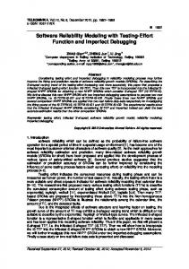
Fig 1. Observed/estimated logistic-exponential and Rayleigh TEF for DS1.
from present & past failure behavior is called predictive
All parameters of other distribution are estimated through LSE. The unknown parameters of Logisticexponential TEF are α=72(CPU hours), λ=0.04847, and k=1.387. Correspondingly the estimated parameters of Rayleigh TEF N=49.32 and b=0.00684/week. Fig.1 plots the comparison between observed failure data and the data estimated by Logistic-exponential TEF and Rayleigh TEF. The PE, Bias, Variation, MRE and RMS-PE for Logisticexponential and Rayleigh are listed in Table I. From the TABLE I we can see that Logistic-exponential has lower PE, Bias, Variation, MRE and RMS-PE than Rayleigh TEF. We can say that our proposed model fits better than the other one. In the TABLE II we have listed estimated values of SRGM with different testing-efforts. We have also given the values of SSE, R2 and MSE. We observed that our proposed model has smallest MSE and SSE value when compared with other models. The 95% confidence limits for the all models are given in the Table III.
validity. This approach, which was proposed by [26], can be represented by computing RE for a data set (18) In order to check the performance of the logisticexponential software reliability growth model and make a comparison criteria for our evaluations [14]. D. SSE criteria: SSE can be calculated as :[17] (19) Where yi is total number of failures observed at a time ti according to the actual data and m(ti) is the estimated cumulative number of failures at a time ti for i=1,2,…..,n.
TABLE-1 COMPARISION RESULT FOR DIFFERENT TEF APPLIED TO DS1
(20) (21) (22) (23)
BIAS
VARIATION
MRE
RMS-PE
PRESENT
0.2243
1.297
0.033
1.27
Rayleigh
0.830337
2.169314
0.052676
2.004112
B. DS2: The dataset used here presented by wood [2] from a subset of products for four separate software releases at Tandem Computer Company. Wood Reported that the specific products & releases are not identified and the test data has been suitably transformed in order to avoid Confidentiality issue. Here we use release 1 for illustrations. Over the course of 20 weeks, 10000 CPU
V. MODEL PERFORMANCE ANALYSIS A. DS1: The first set of actual data is from the study by Ohba 1984 [15].the system is PL/1 data base application software ,consisting of approximately 1,317,000lines of code .During nineteen weeks of experiments, 47.65 CPU hours were consumed and about 328 software errors are removed.
© 2010 ACEEE DOI: 02.ACS.2010.01.254
TEF
9
Proc. of Int. Conf. on Advances in Computer Science 2010
TABLE-II ESTIMATED PARAMETER VALUES AND MODEL COMPARISION FOR DS1
Models
a
r
SSE
R2
MSE
SRGM with Logistic-exponential TEF
578.8
0.01903
2183
0.9889
128.36
353.7
0.08863
7546
0.9615
443.94
SRGM with Rayleigh TEF
459.1
0.02734
5100
0.974
299.98
Delayed S shaped model with Rayleigh TEF
333.2
0.1004
15170
0.9226
892.2
G-O model
760.5
0.03227
2656
0.9865
156.2
Yamada Delayed S shaped model
374.1
0.1977
3205
0.9837
188.51
Delayed S shaped model with Logisticexponential TEF
TABLE III 95% CONFIDENCE LIMIT FOR DIFFERENT SELECTED MODELS(DS1)
a
r
Models Lower
Upper
Lower
Upper
441.5
716
0.01268
0.02538
348.6
569.6
0.01651
0.03817
314.5
392.8
0.07288
0.1044
288.7
377.7
0.07507
0.1258
G-O model
465.4
1056
0.01646
0.04808
Yamada Delayed S shaped model
343.7
404.4
0.1748
0.2205
SRGM with Logistic-exponential TEF
SRGM with Rayleigh TEF
Yamada Delayed S shaped Model with Logsitic-exponential TEF
Yamada Delayed S shaped Model with Rayleigh TEF
© 2010 ACEEE DOI: 02.ACS.2010.01.254
10
Proc. of Int. Conf. on Advances in Computer Science 2010
that SRGM with logistic-exponential TEF have less MSE than other models.
software reliability. Therefore, the optimal software release policy for the proposed software reliability can be formulated as Minimize C(T) subjected to R(t+Δt/t)≥ R0 for C2 > C1, C3 >0, Δt>0, 0 < R0 C1, C3 is the cost of testing per unit testing effort expenditure and TLC is the software life-cycle length. From reliability criteria, we can obtain the required testing time needed to reach the reliability objective R0. Our aim is to determine the optimal software release time that minimizes the total software cost to achieve the desired © 2010 ACEEE DOI: 02.ACS.2010.01.254
When T=0 then m(0)=0 and When T->∞, then And
therefore
is
monotonically decreasing in T. To analyze the minimum value of C(T) Eq. (27) is used to define the two cases of at T=0. 1) if
, then
for 0