2188
OPTICS LETTERS / Vol. 35, No. 13 / July 1, 2010
Wide field-of-view microscope based on holographic focus grid illumination Jigang Wu,1,* Xiquan Cui,1 Guoan Zheng,1 Ying Min Wang,2 Lap Man Lee,2 and Changhuei Yang1,2 1
Department of Electrical Engineering, California Institute of Technology, 1200 E. California Boulevard, Pasadena, California 91125, USA 2
Department of Bioengineering, California Institute of Technology, 1200 E. California Boulevard, Pasadena, California 91125, USA *Corresponding author:
[email protected]
Received March 22, 2010; revised May 19, 2010; accepted May 29, 2010; posted June 7, 2010 (Doc. ID 125762); published June 23, 2010 We have developed a new microscopy design that can achieve wide field-of-view (FOV) imaging and yet possesses resolution that is comparable to a conventional microscope. In our design, the sample is illuminated by a holographically projected light-spot grid. We acquire images by translating the sample across the grid and detecting the transmissions. We have built a prototype system with an FOV of 6 mm × 5 mm and acquisition time of 2:5 s. The resolution is fundamentally limited by the spot size—our demonstrated average FWHM spot diameter was 0:74 μm. We demonstrate the prototype by imaging a U.S. Air Force target and a lily anther. This technology is scalable and represents a cost-effective way to implement wide FOV microscopy systems. © 2010 Optical Society of America OCIS codes: 170.0110, 090.2890, 170.5810.
Automated, high-resolution, and cost-effective wide fieldof-view (FOV) microscopy is highly sought for many applications, such as high-throughput screening [1] and whole-slide digital pathology diagnosis [2]. In a conventional microscope, the FOV is inversely related to the microscope objective’s resolution due to the critical requirement of aberration correction for the whole viewing area. Commercial products for accomplishing wide FOV imaging typically raster scan the target samples under microscope objectives and reconstitute full-view images from multiple smaller images. This approach requires precise mechanical actuation along two axes. Scaling up the FOV for such an approach requires a linear cost increase (add more objectives) or longer scan time. Recently, exciting in-line holography methods [3,4] demonstrated the potential to cover a wide FOV image very cost effectively and without requiring sophisticated optics and mechanical scanning. In-line holography does require excellent raw data quality, as data noise can significantly distort the computed image and deteriorate resolution. To our knowledge, in-line holography’s demonstrated resolution for simple objects is about 1 μm [3]. In this Letter, we report a microscopy technique that employs holography concepts in a different fashion to accomplish wide FOV imaging. Our technique, termed holographic scanning microscopy (HSM), uses a specially written hologram to generate a grid of tightly focused light spots and uses this grid as illumination on the target sample to perform parallel multifocal scanning while the sample is translated across the grid. In comparison to inline holography, the resolution here is fundamentally determined by the focused spot size. Unlike in-line holography, this approach does require mechanical scanning, but the scanning format is a simple one-dimensional (1D) translation. This approach is readily scalable, as we would simply use a large hologram with more projection light spots to accomplish wider FOV imaging. Our HSM prototype demonstration, as shown in Fig. 1(a), used a laser (Excelsior-532-200-CDRH, Spectra Physics, with wavelength of 532 nm and power of 200 mW) as light source. The laser was attenuated, spatial 0146-9592/10/132188-03$15.00/0
filtered, and expanded to be a collimated Gaussian beam with 1=e2 beam diameter of 21:3 mm. We used the center portion of the beam (diameter 12 mm and power 1 mW) as the illumination. A hologram transferred the incoming collimated beam into a grid of 200 × 40 (along the x and the y direction, respectively) focused light spots at a focal length of 6 mm. The spacing between spots was 30 μm. The sample was mounted on a translation stage (LTA-HS, Newport) and positioned under the illumination of the focus grid. An achromatic lens pair (MAP10100100-A, Thorlabs) imaged the focus grid onto the imaging sensor (MotionXtra N3 with 1280 × 1024 pixels and 12 μm pixel size, Integrated Design Tools) with a magnification of 1.6. Note that the aberration induced in the projection lenses is not critical since we only need to differentiate different focus spots, which were well separated (30 μm). A beam block with diameter of 1 mm was positioned at the focus of the lens pair to block the zero-order transmission through the hologram.
Fig. 1. (Color online) (a) System setup of the wide FOV microscope system and (b) scanning mechanism employed for imaging. © 2010 Optical Society of America
July 1, 2010 / Vol. 35, No. 13 / OPTICS LETTERS
In the experiment, we linearly scanned the sample across the focus grid, which was tilted at a small angle with respect to the scanning direction, as shown in Fig. 1(b), and detected the transmission of the foci through the sample. Each focus spot will contribute to a line scan of the sample and a microscopic image can be reconstructed by appropriately shifting and assembling the line scans. This scanning scheme is similar to that of the optofluidic microscope [5], except that here we used a two-dimensional focus grid instead of a 1D aperture array. The focus grid was arranged so that the line scans of the adjacent columns of spots can be directly patched together. The linear scanning scheme has two advantages. First, we can achieve a small sampling distance of the image with relatively large focus spot spacing because of the slight angular tilt geometry. Second, it is simpler and can be much faster than a raster scanning scheme. As shown in Fig. 1(b), the sampling distances in the x and y directions can be written as δx ¼ d sinðθÞ;
δy ¼ v=F;
ð1Þ
where d is the spacing between focus spots, θ is the tilt angle of the focus grid with respect to the sample scanning direction, v is the scanning speed, and F is the frame rate of the imaging sensor. In the experiment, we chose the parameters to be d ¼ 30 μm, θ ¼ 0:025 rad, v ¼ 2:5 mm=s, and F ¼ 3333 frames=s. The exposure time was 7 μs. Thus the sampling distances δx and δy were both 0:75 μm, approximately matching the average focus spot size in our HSM system. Note that a high density of focused light spots is desirable as it would allow us to simultaneously collect more image data. On the other hand, we need to maintain adequate separation between adjacent light spots so that their projections on the sensor can be unambiguously distinguished. Our chosen spacing of 30 μm worked well as a compromise. According to the scanning scheme, the FOV in the x direction is determined by the extent of focus spots in this direction. Because of the linear scanning characteristics, the starting and ending part of the image will have a sawtooth shape, as shown in Fig. 1(b). The effective FOV in the y direction can be calculated by L − H, where L is the scan length and H is the extent of focus spots in the y direction. We used 200 × 40 focused light spots with 30 μm spacing, and a scan length of 6:2 mm for acquiring our images. Thus the FOV was 6 mm in the x direction and 5 mm in the y direction. The acquisition time of the image is determined by the scanning speed and the range of the translation stage, and was calculated to be 2:5 s. We note that the FOV in the x direction can be expanded by simply adding more focused light spots along that direction through the use of a larger hologram. The FOV in the y direction is limited only by the extent to which we are willing to translate our sample along that direction. The key optical component of our HSM system is the hologram. The use of holography to generate tiny focus spots has been reported in the literature [6,7]. Our hologram is technically challenging, as we require it to be capable of rendering tightly focused light spots over a relatively wide area. We implemented a scheme that is capable of patterning such a hologram [shown in Fig. 2(a)]. In this scheme, we employed a specially prepared mask. The mask consisted of a grid of apertures
2189
patterned on a layer of metal film. The aperture diameter was 0:8 μm, and the spacing between adjacent apertures was 30 μm. The metal film was intentionally chosen to be thin (with an optical density of ∼3) so that the incoming collimated light can be transmitted through it and be attenuated. The light transmitted through the apertures, serving as the sample beam, would then interfere with the attenuated collimated light, serving as the reference beam, and project an appropriate pattern onto the holographic plate (VRP, Integraf) for recording. After exposure, the holographic plate was developed and bleached to produce the hologram. During reconstruction, as shown in Fig. 2(b), a conjugated collimated beam can then be transformed into a focus grid, and the focal length is the same as the distance between the holographic plate and the mask during recording. Note that there is a strong zero-order beam during reconstruction that needs to be blocked to enhance the spot pattern contrast in the imaging sensor, as shown in Fig. 1(a). Using the in-line holography scheme, the focal length can be adjusted easily, and a large area of apertures in the mask can be recorded. The effective NA of the recording is ultimately limited by the resolution of the holographic material. Our holographic plate has a resolution of more than 3000 lines=mm, which corresponds to a maximum NA of 0.8. The focus grid was observed under a microscope to measure the focus spot size. Figures 2(d)– 2(f) show microscope images, using a 60× objective, of spots from different region of the focus grid, as indicated in Fig. 2(c). The FWHM spot size was measured to be 0:65–0:80 μm (average of 0:74 μm). The effective NA was ∼0:36, and the Rayleigh range is ∼2:3 μm. The deviation of the experimental NA from the theoretical maximum NA is attributable to recording and developing imperfections. The nonuniform spot intensities of different focus spots were compensated by a normalization procedure during data processing. Note that the spot size in the x direction is larger than that in the y direction. The asymmetric shape of the spot was due to slight misalignment of the mask and holographic plate during the recording process. The simplicity of this recording scheme and its robustness are important, as the method can be used to create
Fig. 2. (Color online) (a) In-line holographic recording scheme for making the hologram, (b) generation of focus grid illumination by holographic reconstruction using the hologram, (c) schematic of the focus grid, and (d)–(f) observation of focus spots from different regions of the focus grid, as indicated in (c), under a microscope using a 60× objective.
2190
OPTICS LETTERS / Vol. 35, No. 13 / July 1, 2010
large format and good quality light-spot-grid holograms. At this point, it is also worth noting that there are other ways to implement focus grid illumination, e.g., by using a microlens array [8]. The challenge of using a microlens array lies in the fact that, to maintain a reasonable NA and high focus-light-spot density, the focal length would have to be very short. For example, for a spacing of 30 μm and NA of 0.36, the microlens would have a diameter of 30 μm and a focal length of ∼40 μm. Aside from fabrication issues related to the difficulty of implementing such small lenses and short focal lengths with good focusing quality, the short focal length is also inconvenient for sample handling. In comparison, our hologram had a much longer focal length of 6 mm. This difference is attributable to the fact that the effective lenses in the hologram can overlap each other, while microlenses simply cannot overlap in a microlens array. In fact, the extent of overlap for our prototype was remarkable. In our prototype, the holographic “lenses” were effectively 4:3 mm in diameter, while the lens-center spacing was 30 μm. To test our prototype system, we acquired images of a U.S. Air Force target and a lily anther microscope slide, as shown in Fig. 3. Figure 3(a) shows the wide FOV image of the U.S. Air Force target with effective FOV indicated by a dashed rectangle. Figure 3(b) shows the expanded view of the region indicated in Fig. 3(a), which contains the smallest feature size with a line width of 2:2 μm (group 7, element 6). Figure 3(c) shows the wide FOV image of the lily anther. Many distinct features, such as carpel, microspore, and petal, of the lily anther can be seen in the image. Small features can also be discerned, as demonstrated in Fig. 3(d), where an expanded-view image of the rectangle area indicated in Fig. 3(c) is shown. We can see that our system can render a wide FOV image and still provide good resolution. The shadow artifacts that are apparent in Fig. 3(b) were caused by crosstalk among the projected transmissions of the light spots. Light spots that were close to the feature edges tend to diffract strongly and introduce light onto regions of the camera that are sampling other spots. These systemic artifacts can be iteratively corrected via postimaging processing. We also note that scan motion nonuniformity (∼0:8 μm) is the cause of the image jitter along the scan direction, as can be seen in some horizontal bars. This issue can be solved by employing a more uniform linear actuation system. Our HSM prototype actually operates in a sub-Nyquist sampling regime. To render full images at the fundamental resolution limit set by the spot size, the sampling increment for both directions should be halved. This can be accomplished by choosing a tilt angle θ of 0:0125 rad and using a scanning speed v of 6666 frames=s. Our achieved resolution with the demonstration operating parameters was 1:5 μm; this is why we were able to discern the smallest individual scale bars (feature width ¼ 2:2 μm) in Fig. 3(b). We note that our system does not contain feedback systems (common in commercial FOV systems) for keeping the sample in focus during scanning. We believe that our HSM design can potentially allow us to solve the axial focus control issue by a different means—by using the hologram to instead project a grid of finite Bessel beams [9], we can potentially image nonflat samples without requiring focus tracking. Finally, we note that the HSM can
Fig. 3. (Color online) (a) Wide FOV image of a U.S. Air Force target, with an effective FOV of 6 mm × 5 mm, as indicated in the large dashed rectangle, (b) expanded view of the smallest feature (groups 6 and 7) of the target, as indicated in (a), (c) wide FOV image of a lily anther, with an effective FOV of 6 mm × 5 mm, as indicated in the large dashed rectangle, and (d) expanded view of the small rectangle area as indicated in (c). S.D., scanning direction.
potentially collect fluorescence images by simply inserting the appropriate filter. In summary, we have shown a wide FOV microscope system based on holographic focus grid illumination. The use of focus grid illumination can effectively provide wide FOV and high-resolution microscopy imaging. We have demonstrated the principle by making a prototype system with an FOV of 6 mm × 5 mm and an acquisition time of 2:5 s. The resolution is fundamentally limited by the spot size—our demonstrated average FWHM spot diameter was 0:74 μm. The prototype system was used to image a U.S. Air Force target and a lily anther for capability testing. This work is supported by Department of Defense grant W81XWH-09-1-0051. The authors acknowledge Richard Cote and Ram Datar from the University of Miami for helpful discussions. References 1. M. Oheim, Br. J. Pharmacol. 152, 1 (2007). 2. J. Ho, A. V. Parwani, D. M. Jukic, Y. Yagi, L. Anthony, and J. R. Gilbertson, Hum. Pathol. 37, 322 (2006). 3. W. B. Xu, M. H. Jericho, I. A. Meinertzhagen, and H. J. Kreuzer, Proc. Natl. Acad. Sci. USA 98, 11301 (2001). 4. S. Seo, T. W. Su, D. K. Tseng, A. Erlinger, and A. Ozcan, Lab Chip 9, 777 (2009). 5. X. Q. Cui, L. M. Lee, X. Heng, W. W. Zhong, P. W. Sternberg, D. Psaltis, and C. H. Yang, Proc. Natl. Acad. Sci. USA 105, 10670 (2008). 6. W. H. Liu and D. Psaltis, Opt. Lett. 24, 1340 (1999). 7. F. Kalkum, S. Broch, T. Brands, and K. Buse, Appl. Phys. B 95, 637 (2009). 8. C. H. Sow, A. A. Bettiol, Y. Y. G. Lee, F. C. Cheong, C. T. Lim, and F. Watt, Appl. Phys. B 78, 705 (2004). 9. J. Durnin, J. J. Miceli, and J. H. Eberly, Opt. Lett. 13, 79 (1988).