Proceedings of ASME-IGTI TURBO EXPO 2004 14-17 JUNE 2004 VIENNA (AUSTRIA)
ASME PAPER 2004-GT-54115 WIDGET-TEMP: A NOVEL WEB-BASED APPROACH FOR THERMOECONOMIC ANALYSIS AND OPTIMIZATION OF CONVENTIONAL AND INNOVATIVE CYCLES Alberto Traverso Aristide F. Massardo TPG-DiMSET Università di Genova Italy
[email protected] [email protected]
Walter Cazzola DICo – Department of Informatics and Communication Università di Milano Italy
[email protected]
ABSTRACT In a deregulated energy market the adoption of multipurpose and flexible software tools for the optimal design and sizing of energy systems is becoming mandatory. For these reasons, we have developed WIDGET-TEMP (Web-based Interface and Distributed Graphical Environment for TEMP, ThermoEconomic Modular Program), a tool which is the result of an interdisciplinary research which applied recent IT innovations such as XML and web-based approaches to the analysis and optimization of energy plant layouts on a thermoeconomic basis. WIDGET provides an interface for remotely accessing the internal thermoeconomic analysis, the full life-cycle cost and investment assessment, which includes the economic impact of environmental costs due to pollutant emissions. This approach reduces the requirements for the local machine in terms of processor time and memory, and allows users to exploit the tool just when needed. An initial functional productive diagram of the plant is now automatically drawn and is available to the user on a visual basis. We present a general description of the tool organization and outline the approach for modeling the technical performance and cost of the component. Then, we describe the latest upgrades of TEMP, and report the new gas turbine cost equations. Finally, the tool is applied to a conventional simple and combined cycle, showing both the usability of the new tool and the reliability of the results. INTRODUCTION Whenever a new energy conversion process has to be designed or upgraded, the frequently asked questions are: what type, how much? The basic features that can make the difference are, of course, the performance and the cost. Then,
Giovanni Lagorio DISI – Department of Informatics and Computer Science Università di Genova Italy
[email protected]
once the basic layout has been decided and the preliminary design point settled, other considerations about reliability, maintainability, availability can lead to continuous improvements of the power plant and its organization. However, the original choice influences all the following developments and should be carefully taken. In this respect, tools that can provide estimates of the technical and economic performance of different plant layouts become very helpful. WIDGET-TEMP is a new software environment aimed at the thermoeconomic analysis and optimization of conventional and innovative energy systems at on-design conditions. The software represents the latest evolution of the TEMP (ThermoEconomic Modular Program) code, developed over the last ten years by the TPG. The TEMP had wide capabilities for the thermoeconomic analysis of power plants and it was used for several research works and publications [1-9]. The major limitations of TEMP derived from its implementation using the FORTRAN language of the source code. In fact, this affected the usability and user-friendliness of the tool, which could be effectively exploited only by experienced users. No visual interface was available and the input/output was managed through numerical files. This required a long training/learning time for new users, who could easily make mistakes in the definition of the plant layout and in the interpretation of the results. This was the motivation for the development of WIDGET-TEMP. The WIDGET web-based approach allows users to exploit all the TEMP potentialities directly from their web browser. The TEMP can now be run locally or, alternatively, on a remote machine, which is accessed via Internet. The WIDGET interface provides the possibility of building up and configuring various types of power plant in a visual environment. So, new users can now have a much more straightforward approach to the tool, and time can be saved both in the definition of the 1
Copyright © 2004 by ASME
energy system layout and in the visualization of the simulation results. THE TEMP THERMOECONOMIC APPROACH Systems for converting energy, even the most complex, can be specified using a limited set of basic components (compressors, pumps, and so on). In this respect, the development of a new software tool for simulating energy systems must ensure good modeling flexibility and extendibility, so that a wide range of plant configurations can be easily handled. These requirements led to the adoption of a modular structure for TEMP [2]. The TEMP looks at the system as a generic process, and analyzes and optimizes it regardless of its particular layout. The original TEMP simulation engine has been significantly improved [1-4], and currently TEMP is provided with about sixty components. The most significant are reported in Table 1. All the components are organized in a library, which can be extended by users without modifying the “core” of the code. Figure 1 reports the conceptual organization of TEMP and how it interacts with WIDGET: TEMP solves the engineering problem and exchanges with WIDGET the input for and the output of the thermoeconomic analysis. In TEMP, each component is defined by three subroutines, which describe its thermodynamic, exergetic and thermoeconomic properties at on-design conditions. The subroutines are executed according to the following three cascaded steps: Thermodynamic analysis Exergy analysis Thermoeconomic analysis In the thermodynamic analysis, the physical plant layout defined by the user is solved iteratively, and the thermodynamic performance, in terms of efficiency, heat and power, found. Moreover, the properties of each flow stream, such as mass flow, pressure, temperature, and composition, are calculated. The exergy analysis subroutines are sequentially called: they provide a complete description of the irreversibilities and exergy streams in the plant. Finally, the thermoeconomic subroutines automatically construct the functional productive diagram of the cycle (briefly, “functional diagram”), which is necessary for the complete thermoeconomic analysis of the plant. As a result, the capital costs of all the components (see Appendix A) and the specific and marginal costs (monetary and exergetic) of each flow stream are calculated. Environmental costs related to pollutant emissions can also be included in the analysis [4][10]. The results allow the user to obtain the details of the behavior of the plant as well as its global technical and economic performance. Moreover, the thermoeconomic diagnostics provided by the exergoeconomic analysis [11], performed within the thermoeconomic analysis, provides a deeper and more complete understanding of the system. Recently, the assessment of the balance of the plant and investment profitability have been enhanced, through the introduction of the through-life cost analysis, which allows the
user to calculate the “global” economic parameters of the plant, such as the net present value (NPV) or the internal rate of return (IRR) [5]. Optimization can be applied to the whole system, and different objective functions, such as the best thermodynamic efficiency or the best economic performance (i.e. minimum cost of electricity, maximum IRR), can be pursued. Initially, Lagrangian formulation of the optimization problem was used, which, unfortunately, made the system stiff and insufficiently flexible [12]. The TEMP code, instead, started with the Direct Thermoeconomic Optimization (D.T.O.), where a non-linear algorithm of optimization is directly applied to the objective function, without the intermediate step represented by the Lagrangian multipliers. Nevertheless, the internal economy (properly “thermoeconomic internal analysis”) is calculated separately. Table 1 – Main components available in TEMP Conventional Advanced Compressor CH4 Steam Reformer Combustor
CO2 Separation Unit
Turbine
Fuel Cell SOFC
Steam turbine
Fuel Cell MCFC
HRSG Heat Recovery Steam Generator
Flue Gas Condenser
Steam Condenser
Saturator
SCR Selective Catalytic Reduction
Biomass Gasifier
WIDGET
ECONOMIC SCENARIO
PLANT PHYS ICAL DIAGRAM
CALCULATION OPTIONS
PLANT DATA
RES ULTS
PLANT FUNCTIONAL DIAGRAM
THERMODYNAMIC EX ERGY THERMO ECONOMIC
OPTIMIZATION TOOL
ANALYS ES
COMPONENT LIB RARY
Figure 1 WIDGET-TEMP conceptual scheme
2
Copyright © 2004 by ASME
Figure 2 WIDGET-TEMP: coding of project file
WIDGET: IMPROVING THE AVAILABILITY AND USABILITY OF TEMP Albeit the TEMP simulation engine has evolved steadily, its user-friendliness has not been enhanced accordingly. In order to run a simulation, users must write a text-file consisting of a series of figures, which describes the basic components of the plant, their properties and their interconnections. Basically, each component is identified by an integer and its properties are represented by a series of floating-point numbers. An example can be seen in Figure 2, which shows how a piece of a plant is coded. The upper part of the figure shows how the plant is designed inside WIDGET, the lower part shows a snippet from the corresponding input file for TEMP. Each row of the input file corresponds to a component, and each row consists of four sections: comment, kind, connections and properties. The comment section is just what you expect: a comment, which is ignored by TEMP. The type is a positive integer that identifies a class of components; in the example three components are shown: an air inlet (identified by 19), a compressor (identified by 14) and a gas expander (identified by 16). The connection section of each component consists of a series of integers, one for each port of the component. These integers specify the connection each port is connected to. That is, each connection is identified by a positive integer and using the same number in the two places corresponding to the ports specifies a connection between two ports. In the example, the connection between the air inlet and the compressor is specified by the number “1” and the connection between the compressor and the expander by the number “3”. The big arrows in the figure show this correspondence.
The last section specifies the properties for each component as a series of floating point numbers. Each component has a different set of properties, so it is very difficult to remember what is needed and in what order. Instead, as the figure highlights, WIDGET lists the property names in a panel where the user has only to insert the values (and can check the online help for getting further insights if necessary). It is fairly evident that designing and coding even a simple plant in this way is a difficult and error-prone process. So many variables and properties are involved for each component that using them in a consistent way is rather complex for a nonexpert user. Moreover, the result of a simulation is a text file as well, which is full of numerical information correlated to several components or streams of the input plant. Basically, before the development of WIDGET, the users had to translate their intuitive idea of a plant into a numberbased representation (to be processed by a FORTRAN program) and then, to map the result on their original vision of the plant without any graphic support. Although this was the only viable option when the project started, this approach forces the user to think as a computer and requires a deep knowledge of the inner working of the program to get sensible results. Nowadays, technology has evolved to the point in which users can think in application domain terms only, without bothering with the error-prone paradigm shift required before. WIDGET is a graphical front-end to TEMP which provides users with a user-friendly interface to design their plants. They can then “draw” them using a library of basic components, set their properties and connect them with few mouse clicks. WIDGET performs some consistency checks during the design of a plant; for instance, users are prevented from connecting together incompatible ports (e.g., a power 3
Copyright © 2004 by ASME
input to a water input). When a plant is properly connected, WIDGET can run TEMP to carry out the simulation. Then, the results of the simulation are mapped on the graphical diagrams simplifying their interpretation. At any moment, the user can customize the visualization by choosing which results provided by TEMP are to be shown; as is highlighted in Figure 5, the user can decide which type of result to show, and in what order. The translation back and forth to the text-based representation remains, but now it is performed by WIDGET, which hides all the details of this translation behind a graphical front-end. WIDGET has been designed as a separate program, which wraps a graphical interface around TEMP for different reasons: 1. by adopting a Java-based technology, WIDGET can be run on any machine that can run Java, i.e., every modern computer (while TEMP can currently run only on Windows machines); 2. by adopting client/server architecture, interoperability among different combination of operating systems and hardware is granted. In this architecture, TEMP is the server process, and each instance of WIDGET is a client. Hence, while TEMP has still to be run on a Windows-based machine, users can now use TEMP remotely with any kind of machine (e.g., Linux-box or Macintosh) through WIDGET; 3. being a Java applet, WIDGET can be used inside any Java-enabled browser without requiring any software installation or configuration. We can summarize the novel features introduced by WIDGET as open and flexible architecture, a remote access to TEMP and, last but not least, an automatic generation of a graphical view for the functional diagrams. WIDGET AS OPEN ARCHITECTURE As said before, WIDGET is a program that is completely separated from TEMP. Yet, WIDGET must know which components TEMP handles, how to display them and how to check their consistency. Not wanting to hard-code the properties of each component inside WIDGET, we had to find a lingua franca to share the TEMP knowledge base with WIDGET. It turned out that XML [21], being an extensible markup language, is perfect for this task. XML is a standard language for describing other languages, which lets you design your own dialect for different types of data. In our case, we defined an XML dialect that let the TEMP developer describe every aspect of a component (its inputs/outputs, its properties and so on) known to TEMP. Therefore, a graphical representation must also be associated with the component by other means. Each component can be used by WIDGET to build two kinds of diagram: the physical and the functional view. Because the appearance of a component can differ in these two diagrams, we have associated each component with two external files that contain its vectorial graphical representation to be used in the physical and in the functional diagram respectively.
Figure 3 “Compressor”
Snippet of XML file for module
The consistency between the graphical representation and the data specified inside the XML files can be automatically checked by a special tool provided as a support for future extensions of TEMP. When these data are consistent the tool writes a compressed representation of all the TEMP components inside a file that is then used by WIDGET. Note that this tool has to be used by TEMP developers only when they need to change some aspects of an existing component or add a new component to TEMP. The end-users do not have to use any particular tool, except WIDGET itself. This approach is very flexible, because TEMP developers never need to change WIDGET in order to change or extend the component base library. They just need to write the description of the new component into an XML file, to draw its graphical representation in the two files (as explained before), and run the tool once. Figure 3 shows the XML file that describes the Compressor as an example. CREATING THE FUNCTIONAL DIAGRAM VIEW The automatic generation of a functional diagram is a major enhancement in analyzing a plant from a thermoeconomic point of view. The first time TEMP is (successfully) run on a plant, a functional diagram is created from the physical diagram and the results of the simulation. The former is used to lay out the components in the functional view; the latter describes the connection between ports (connections defined in the functional view are a superset of the ones defined in the physical view). While this automatically generated diagram is not usually as clean as one would like it to be, it is a well-known open research problem [22] to lay out a set of “connections” without creating useless intersections. Therefore the diagram could not be as clear as expected without fixing something. However, users can clean up this diagram moving components and connections “by hand”. WIDGET remembers all these manual changes so, in later runs of the simulations, 4
Copyright © 2004 by ASME
WIDGET creates the new functional view diagram as close as possible to the previous one, retaining its “proper” appearance. REMOTING TEMP One of our initial goals was to make TEMP remotely usable without affecting its source code. We have achieved this target by wrapping TEMP inside a Java program. That is, TEMP is still a Windows program that reads its input from files and writes its output to other files but, when used through WIDGET, it is invoked by a Java program that writes the input files before invoking TEMP and captures its output, sending it to the remote Java applet which has asked to run the simulation. So, even if we always talk about WIDGET as a single program, it really consists of two parts: a (small) part that runs as a server on the Windows machine and another (big) part that runs as a client inside the user’s web-browser. The latter part is the only one the end-users directly interact with. WIDGET-TEMP AT WORK: SIMPLE CYCLE AND COMBINED CYCLE ASSESSMENT WIDGET-TEMP capabilities have been tested for the V94.2 simple cycle and 1.V94.2 combined cycle, taken as an example to show the features of the new tool. Table 2 reports the basic features of the plants, together with the main data calculated by WIDGET-TEMP. The comparison of the data published in open literature and the calculated data shows a
good accuracy in the results, both from a thermodynamic (error < 1% ) and economic (error < 8%) point of view. The costs have been estimated with the cost equations in Appendix A and the heat recovery system costs given in [19]. The tool has also been tested against other combined cycles not reported here, giving good thermodynamic results and capital cost estimations within a ±15% error range. Table 2 1.V94.2 dual pressure combined cycle data [18] and WIDGET-TEMP results
Net Power [kW] Efficiency [%] GT Pressure ratio Intake air [kg/s] Turbine Outlet Temperature [°C] Capital Cost [106 $] Specific Cost [$/kW]
V94.2 Gas Turbine Available WIDGETdata TEMP results 159400 159380 34.4 34.4 11.4 11.4 509 505
1.V94.2 Combined Cycle Available WIDGETdata TEMP results 232900 51.7 11.4 509
235000 51.23 11.4 505
547
545
547
552
24.7 155
26.3 164
103.87 446
102.5 436
In the following images (Figures 4-8), examples of WIDGET-TEMP windows are reported. They report examples of physical diagrams and functional diagrams, with the main properties, such as temperature, pressure, capital costs of the components, specific costs of the streams, displayed.
Figure 4 WIDGET-TEMP: V94.2 simple cycle physical diagram with temperatures [°C] and pressures [bar] 5
Copyright © 2004 by ASME
Figure 5 WIDGET-TEMP: V94.2 simple cycle physical diagram with component costs [$]
Figure 6 WIDGET-TEMP: V94.2 simple cycle functional diagram with stream specific cost [$/kJ] (negentropy streams are also reported) 6
Copyright © 2004 by ASME
Figure 7 WIDGET-TEMP: 1.V94.2 combined cycle physical diagram The recent upgrades of TEMP capabilities for the full life cycle analysis and the update of cost equations improved the accuracy of the results obtained. ACKNOWLEDGMENTS The authors wish to thank Giovanna Massetti of TPG for her active contribution to the development of WIDGET-TEMP, Massimo Ancona of the Department of Informatics and Computer Science of Genova for believing in interdisciplinary collaboration and research. The second author wishes to thank Dr. Alessio Agazzani, who started TEMP development many years ago as a Ph.D student. Figure 8 WIDGET-TEMP: 1.V94.2 combined cycle functional diagram. Detail of the 2LP Heat Recovery CONCLUSIONS WIDGET-TEMP represents a novel web-based tool for the thermoeconomic analysis and optimization of complex energy systems. It includes all the capabilities of the original TEMP code, now available through every web browsers. This reduces the use of local resources (processor and memory) and makes the tool available for a very wide range of users. The visual interface allows the training time for new users to be significantly reduced and the results to be more straightforward interpreted. The functional productive diagram of the plant is automatically drawn and available to the user.
APPENDIX A: GAS TURBINE COST EQUATIONS The cost functions for gas turbine simple cycles have been updated to the latest cost data available in open literature (Figure 9). The original form presented in [2] has been modified to improve both the power range of validity of such correlations and the management of non-conventional fluids, such as gas and water/steam mixtures. Table 3 presents the gas turbines considered for cost equation data-fitting. The first part of the columns refers to the data taken from [18] and used as a reference, while the second part of the columns refers to the performance inferred with WIDGET-TEMP. The blade-cooling model employed here is a simplified version of the complete model in [20]. The present model is based on the blade uniform temperature approach and considers the expander as a whole (no distinction between stages). The cooling flow requirement is then calculated as a 7
Copyright © 2004 by ASME
result, and it is considered to be bled from the last compressor stage. 900
(m out ⋅ Vout ) Ξ combustor = cc1 (m out ⋅ Vout ) ref
m air R in Tin Pin ⋅ mcr cc5
c4 ⋅ β ln(β) 1 - ηpolC c 2 ref
(
)
cc3⋅ Tout - cc4 T ref 1 ⋅ ⋅ 1. + e out cc2 dPp
t5
(m out ⋅ Vout ) Ξ turbine = t1 1. + e (m out ⋅ Vout ) ref
Tin t3⋅ T ref in
Pow el Ξ generator = g1 Pow el ref
Symbols dPp percentage pressure drop m mass flow P pressure Pow power R gas constant T temperature V specific volume pressure/expansion ratio β efficiency η capital cost Ξ
- t4 ⋅
ln(β ) 1 - ηpolT
(
)t 2
800
(1)
Gas Turbine Price ($/kW)
m R in Tin Ξ compressor = c1 air Pin ⋅ m cr
c3
(2)
(3)
700
y = -98.328Ln(x) + 1318.5
600 500 400 300 200 100 0 0
g2
50000
100000
Table 4 Coefficients of the gas turbine cost function (dimensionless, unless reported) c1 [$] c2 c3 c4 cc1 [$] cc2 cc3 cc4 cc5 Pref [Pa] Tref [K] mref [kg/s]
The coefficients used in the cost functions are reported in Table 4. The cost obtained from the equations was increased by a factor of 1.26, which takes into account the cost for electrical equipment and control instrumentation.
5095.9 0.15 0.85 0.3 1857.0 0.995 5.479 34.36 0.6 101325 288.15 1.0
Makila TI (Turbomeca) ST18A (Pratt & Whitney) UGT-2500 (Maskproekt) ST40 (Pratt & Whitney) Taurus 60 (Solar) Tempest (Alstom) Titan 130 (Solar) UGT-15000+ (Maskproekt) LM2500PE (ISH) GT10C (Alstom) RB211-6761 DLE (Rolls Royce) PG6561B (Hitachi) LM6000PD (GE) Trent 50 (Rolls Royce) V64.3A (Siemens) PG6111(FA) (GE) GT11N2 (Ansaldo) PG9171E (Hitachi) V94.2 (Siemens) PG7241FA (GE)
1988 1995 1992 1999 1993 1995 1998 1998 1976 1999 2000 1996 1994 1996 1996 2003 1993 1987 1981 1994
[kW] [$/kW] 1050 838 1960 611 2850 456 4040 446 5500 355 7910 373 14250 335 20000 275 22800 402 29060 292 32120 321 39620 255 42330 241 51920 312 67400 236 75900 245 116500 169 123400 165 159400 155 171700 182
Cost [$] 880000 1200000 1300000 1800000 1950000 2950000 4770000 5500000 9175000 8490000 10300000 10100000 10200000 16200000 15900000 18600000 19700000 20400000 24700000 31250000
Powref [kW] 1.0 Rref [J/kgK] 289.2 0.9586 mcrref
Calculated
Pressure Exhaust Intake Ratio Efficiency Temp. Air [%] 9.6 14.0 12.0 16.9 12.5 13.7 16.1 19.4 18.4 18.0 21.5 12.0 29.3 32.0 15.8 15.6 15.5 12.3 11.4 16.0
27.1 30.2 27.5 33.1 30.4 31.2 35.0 34.2 36.8 36.0 39.3 31.9 41.1 42.2 33.8 35.0 33.9 33.8 34.4 36.2
5979.1 0.29 4.185 23.60 0.75 1030.9 0.72
t1 [$] t2 t3 t4 t5 g1 [$] g2
Data (Gas Turbine World 2003) Gas Turbine
200000
Figure 9 2003 specific Gas Turbine cost trend against the net power output (data from [18])
Subscripts in inlet out outlet cr critic air air ref reference pol polytropic el electrical
Specific Cost Year Power
150000
Plant Output (kW)
(4)
TIT
Blade Cooling
[°C] [kg/s] [°C] [% intake] 505 5.4 995 8.9 532 8.0 1140 11.0 435 14.9 933 8.2 544 13.9 1220 12.1 510 21.9 1080 10.0 537 29.8 1150 10.9 482 49.8 1122 10.7 412 70.0 1040 10.3 520 74.0 1234 12.0 518 91.0 1218 11.8 503 94.4 1260 12.2 532 144.3 1120 10.4 452 126.0 1270 13.1 312 152.9 1279 13.8 583 191.9 1288 12.3 603 202.8 1322 12.6 530 400.0 1185 11.4 538 403.7 1152 10.6 547 509.0 1155 10.5 601 444.5 1350 12.7
ηCpol
Combustor ηTpol Press. drop
0.881 0.886 0.884 0.893 0.892 0.893 0.902 0.904 0.903 0.903 0.917 0.891 0.928 0.922 0.902 0.895 0.895 0.899 0.905 0.906
0.834 0.823 0.833 0.834 0.834 0.831 0.851 0.842 0.852 0.847 0.862 0.844 0.868 0.860 0.840 0.842 0.838 0.862 0.874 0.848
[%] 9.0 6.0 5.0 9.0 6.0 5.0 5.0 5.0 5.0 5.0 5.0 5.0 5.0 5.0 5.5 5.0 5.0 5.0 5.0 5.0
Table 3 Gas Turbine Data from [18] and calculated with WIDGET-TEMP 8
Copyright © 2004 by ASME
Vref can be calculated with the perfect gas law. The coefficients were obtained through an optimization procedure that minimized the quadratic error (the function “Lsqcurvefit” available in Matlab© Optimization Toolbox [13] was used. The algorithm is presented in [15][16]). With these new cost equations, the range of validity of the cost equations was extended from 1MW to 170MW (tuning range); however, such cost equations were successfully extrapolated up to 300MW, always keeping the estimation error within ±15%. The average error within the tuning range was lower than 13% (Figure 10). It is worth remembering that the subdivision of a single gas turbine into its basic components is useful to provide the code with the necessary flexibility to study innovative cycles, including intercooled or re-heated gas turbine [3], humid air cycles [5], CO2 separation gas turbine plants [6], and others, where these basic devices can be assembled in nonconventional ways. 4.E+07
4.E+07
Cost Equation Estimation [$]
3.E+07
3.E+07
2.E+07
2.E+07
TEMP WIDGET-TEMP Gas Turbine World 2003 -15% Gas Turbine World 2003 +15% Gas Turbine World 2003
1.E+07
5.E+06
0.E+00 0.E+00
5.E+06
1.E+07
2.E+07
2.E+07
3.E+07
3.E+07
4.E+07
Actual Cost [$]
Figure 10 Gas Turbine Cost: new cost equations compared to the previous ones [2] REFERENCES [1] A. Agazzani, A. F. Massardo, A. Satta, 1995, “Thermoeconomic Analysis of Complex Steam Plants”, ASME Paper 95-CTP-38. [2] A. Agazzani, A. F. Massardo, 1997, “A Tool for Thermoeconomic Analysis and Optimization of Gas, Steam, and Combined Plants”, Journal of Engineering for Gas Turbine and Power, 119, 885-892. [3] A.F. Massardo, M. Scialò, 2000, “Thermoeconomic Analysis of Gas Turbine Based Cycle”, Journal of Engineering for Gas Turbine and Power, 122 , 664-671. [4] A. Agazzani, A.F. Massardo, C.A. Frangopoulos, 1998, “Environmental Influence on the Thermoeconomic Optimization of a Combined Plant with NOx Abatement”, Journal of Engineering for Gas Turbine and Power, 120, 557565. [5] A. Traverso, A. F. Massardo, 2002, “Thermoeconomic Analysis of Mixed Gas-Steam Cycles”, Applied Thermal Engineering, Elsevier Science, 22 (2002), 1-21.
[6] M. Bozzolo, M. Brandani, A. F. Massardo, A. Traverso, “Thermoeconomic Analysis of a Gas Turbine Plant with Fuel Decarbonisation and CO2 Sequestration”, ASME Paper GT2002-30120 (accepted for Transactions), Best Paper Award ASME IGTI 2002. [7] Research contract n. PRC0S090.1, between ENEL e DIMSET, 2001,“High temperature fuel cell hybrid system and humid air cycle modeling”. [8] Research contract between Ansaldo Ricerche e DIMSET 2002, “Microcogen”. [9] “Thermodynamic Cycles using Liquid Diluent”, January 2003, US Patent pending, assigned to VAST Power Systems. [10] A. Traverso, M. Santarelli, A. F. Massardo, M. Calì, 2002, “A New Generalised Carbon Exergy Tax: an effective rule to control global warming”, ASME Paper 2002-GT-30139 (accepted for Transactions). [11] G. Tsatsaronis, M. Winhold, 1985, “Exergoeconomic Analysis and Evaluation of Energy Conversion Plants. I- A New General Methodology”, Energy, Vol. 10, No. 1, pp. 69-80. [12] C. A. Frangopoulus, 1983, “ Thermoeconomic Functional Analysis: a Method for Optimal Design or Improvement of Complex thermal System”, Ph. D. Thesis, Georgia Institute of Technology, Atlanta, GA. [13] The Mathworks, “Matlab User Manual”, Release 13.0.1, 2003 [14] Y. El-Sayed, M. Tribus, 1983, “Strategic Use of Thermoeconomics for System Improvement”, Journal of Engineering for Power, 92, 27-34. [15] T. F. Coleman, Y. Li, 1994, “On the Convergence of Reflective Newton Methods for Large-Scale Nonlinear Minimization Subject to Bounds”, Mathematical Programming, Vol. 67, Number 2, pp. 189-224. [16] T. F. Coleman, Y. Li, 1996, “An Interior, Trust Region Approach for Nonlinear Minimization Subject to Bounds”, SIAM Journal on Optimization, Vol. 6, pp. 418-445. [17] A. Bejan, G. Tsataronis, M. Moran, "Thermal Design & Optimisation" Wiley-Interscience Publication, John Wiley & Sons Inc., 1996. [18] Gas Turbine World, 2003, “ Gas Turbine World 2003 Handbook”, Pequot Publishing Inc. [19] Foster-Pegg R.W., 1986, “Capital Cost of Gas-Turbine Heat-Recovery Boilers”, Chemical Engineering, Vol. 93, n. 14, pp. 73-78. [20] L. Torbidoni, A. F. Massardo, 2002, “Analytical blade row cooling model for innovative gas turbine cycle evaluations supported by semi-empirical air cooled blade data”, ASME Paper 2002-GT-30519 (accepted for Transactions). [21] World Wide Web Consortium. Extensible Markup Language (XML) 1.0. W3C Recommendation available at http://www.w3.org/TR/REC-xml , February 1998. [22] Daniel Bienstock, 1990, “Some provably hard crossing number problems”, Proceedings of the sixth annual symposium on Computational geometry, ACM Press.
9
Copyright © 2004 by ASME