Pogosyan, and K. B. Wolf, ''Wigner functions for curved spaces. I. On hyperbo- .... Alonso, Pogosyan, and Wolf ...... Ozaktas, R. Simon, and K. B. Wolf, J. Opt. Soc.
JOURNAL OF MATHEMATICAL PHYSICS
VOLUME 44, NUMBER 4
APRIL 2003
Wigner functions for curved spaces. II. On spheres Miguel Angel Alonso, George S. Pogosyan,a) and Kurt Bernardo Wolf Centro de Ciencias Fı´sicas, Universidad Nacional Auto´noma de Me´xico, Apartado Postal 48-3, Cuernavaca, Morelos 62251, Me´xico
共Received 12 November 2002; accepted 10 December 2002兲 The form of the Wigner distribution function for Hamiltonian systems in spaces of constant negative curvature 共i.e., hyperboloids兲 proposed in M. A. Alonso, G. S. Pogosyan, and K. B. Wolf, ‘‘Wigner functions for curved spaces. I. On hyperboloids’’ 关J. Math. Phys. 43, 5857 共2002兲兴, is extended here to spaces whose curvature is constant and positive, i.e., spheres. An essential part of this construction is the use of the functions of Sherman and Volobuyev, which are an overcomplete set of plane-wave-like solutions of the Laplace–Beltrami equation for this space. Rotations that displace the poles transform these functions with a multiplier factor, and their momentum direction becomes formally complex; the covariance properties of the proposed Wigner function are understood in these terms. As an example for the one-dimensional case, we consider the energy eigenstates of the oscillator on the circle in a Po¨schl–Teller potential. The standard theory of quantum oscillators is regained in the contraction limit to the space of zero curvature. © 2003 American Institute of Physics. 关DOI: 10.1063/1.1559644兴
I. INTRODUCTION
In the first part of this series1 we proposed a generic form for the Wigner quasiprobability distribution function defined in terms of the generalized basis of plane waves; this form may be extended in a natural way to curved configuration spaces, provided that an analogous basis of plane-wave-like solutions can be found on those manifolds; the new functions will correspondingly endow their argument and index with the physical meaning of position and momentum. Although one may think to generalize the Wigner function to any manifold, the hyperboloid and the sphere are the two simplest cases to start such a study. In Ref. 1 we considered spaces of constant negative curvature, i.e., the upper sheet of a two-sheeted hyperboloid, where the basic plane waves were the set of Shapiro functions.2 That Wigner function has the desired marginal projections, and its properties of covariance under rotations and hyperbolic translations were shown to stem from those of the Shapiro functions. The goal of this second part is the study of the Wigner function on spaces of positive constant curvature, i.e., on spheres. As was the case in Ref. 1, the generalization offered in our approach results from recognizing that the Wigner function on flat phase space (p,x)苸R2D , 3 in addition to its usual expression as a single integral, can be written also in the following twofold integral form with a Dirac ␦,
1
W RD 共 f ,g 兩 x,p兲 ª
共 2 兲D
⫽
1 共 2 兲D
冕 冕
RD
d D zf 共 x⫺ 21 z兲 * e ⫺ip•zg 共 x⫹ 21 z兲
RD
d D x⬘
冕
RD
d D x⬙ f 共 x⬘ 兲 * g 共 x⬙ 兲 p共 x⬘ 兲 ␦ D 共 x⫺ 21 共 x⬘ ⫹x⬙ 兲兲 p共 x⬙ 兲 * , 共1兲
a兲
Permanent address: Laboratory of Theoretical Physics, Joint Institute for Nuclear Research, Dubna, Russia and International Center for Advanced Studies, Yerevan State University, Yerevan, Armenia.
0022-2488/2003/44(4)/1472/18/$20.00
1472
© 2003 American Institute of Physics
Downloaded 03 Apr 2003 to 132.248.33.128. Redistribution subject to AIP license or copyright, see http://ojps.aip.org/jmp/jmpcr.jsp
J. Math. Phys., Vol. 44, No. 4, April 2003
Wigner functions for curved spaces. II. On spheres
1473
where the function p(x) and its complex conjugate p(x) * , whose argument and index variables bind the position and momentum variables, are the plane waves
p共 x兲 ªexp共 ip•x兲 ,
⫺⌬ 共 x兲 ⫽ p 2 共 x兲 ,
共2兲
where pª 兩 p兩 , and which are solutions of the Helmholtz 共Laplace–Beltrami兲 equation on flat space. Momentum p has units of inverse length when ប⫽1; in optics, p is the wave number of light. The form 共1兲 of the Wigner function again suggests its generalization to the sphere S D through replacing the integration over flat space ( 兰 RD d D x) by an integration over the new D-dimensional manifold ( 兰 S D dx), replacing the plane waves p(x) of flat space by plane-wavelike solutions of the Laplace–Beltrami equation on that manifold, and replacing the Dirac delta ␦ D (x⫺ 21 (x⬘ ⫹x⬙ )) in 共1兲 by an appropriate distribution on the sphere. The new reproducing kernel should guarantee that, if x⬘ and x⬙ are on the manifold, then x should lie halfway along a geodesic. In flat space, the transformation between the position and momentum representations arises from the basis of plane wave functions 共2兲 that defines the Fourier transform; on the hyperboloid, it is a Mellin transform. Here, this transform will relate wave functions on the sphere with functions over a momentum space, through a summation over the discrete values that the wave number can have on the sphere, and an integral over the directions of the plane waves. Both the hyperboloid and the sphere are characterized by the radius R 共curvature ⫾1/R), which will serve as the contraction parameter whose limit R→⬁ represents flat space, and where the traditional phase space and Wigner function are recovered. Let us stress that, unlike previous studies where the sphere is the symplectic manifold on which the Wigner function is drawn, as in the cases for spin4 and finite systems,5,6 or of the Wigner function defined on the coadjoint orbits of a Lie algebra7 which may have a similar or more complicated topology, this Wigner function describes wave fields whose configuration space is the sphere. Also, we distinguish the present case from other previous definitions describing Helmholtz wave fields in flat free space, where momentum is constrained to the so-called Descartes sphere of ray directions.8 In Sec. II we concentrate the necessary definitions and relevant properties of these planewave-like solutions, and our understanding of the momentum space conjugate to the sphere. In Sec. III we develop the new Wigner function on the direct product phase space, making explicit its covariance properties and its contraction limit. As in Ref. 1, we illustrate some of these results in Sec. IV with an example: the harmonic oscillator analog on the circle (D⫽1) that corresponds to the bounded-interval Po¨schl–Teller potential. In Sec. V we recapitulate our results in the context of other approaches in the literature. II. SPHERICAL SPACES AND MOMENTUM
We follow the plan of Ref. 1 to present the Laplace–Beltrami operator on the curved space— here a D-dimensional spherical manifold—and its corresponding basis of plane-wave functions.9,10 This is the basis we choose to define the momentum manifold that will appear in the definition of the Wigner function in the next section. A. Laplace–Beltrami operator on the sphere
Consider the D-dimensional manifold of a sphere S D of radius R⬎0, embedded in the ambient space x苸RD⫹1 , 兩 x 兩 2 ªx 20 ⫹x2 ⫽R 2 ,
2 x2 ªx 21 ⫹x 22 ⫹¯⫹x D .
共3兲
The isometry group of the manifold of x’s is the real orthogonal group in D⫹1 dimensions; for simplicity we disregard reflections and use the proper rotation group SO(D⫹1). This will replace the Euclidean isometry ISO(D) ⫹ of flat configuration space. The standard realization of the Lie algebra so(D⫹1) by generators of rotations of the ambient (D⫹1)-dimensional space 共3兲, is
Downloaded 03 Apr 2003 to 132.248.33.128. Redistribution subject to AIP license or copyright, see http://ojps.aip.org/jmp/jmpcr.jsp
1474
J. Math. Phys., Vol. 44, No. 4, April 2003
Alonso, Pogosyan, and Wolf
M j,k ªx j x k ⫺x k x j ,
共4兲
j,k⫽0,1,2,...,D.
D is (R ⫺2 times兲 the second-order invariant Casimir The Laplace–Beltrami operator on S ⫹ operator, namely,
⌬ LBª
1 1 M2 . 2 C⫽ 2 R R 0⭐ j⬍k⭐D j,k
兺
共5兲
The spectrum of the Casimir operator of so(D⫹1) is well known to be the lower bound, discrete but infinite set of values ⌺ 共 C兲 ⫽ 兵 ᐉ 共 ᐉ⫹D⫺1 兲 兩 ᐉ苸Z ⫹ 0 其,
Z⫹ 0 ª 兵 0,1,2,... 其 .
共6兲
Corresponding to each value of ᐉ there is a unitary irreducible representation belonging to the most degenerate 共also called most symmetric兲 series, which is of finite dimension 关 2ᐉ⫹1 in so(3) for D⫽2]. The free wave functions on the sphere are the solutions to the Laplace–Beltrami equation characterized by those eigenvalues 共6兲, that we choose to write as ⌬ LB f 共 x兲 ⫽⫺
冋 冉 冊册
D⫺1 ᐉ 共 ᐉ⫹D⫺1 兲 f 共 x兲 ⫽⫺ p 2 ⫺ R2 2R
pª 关 ᐉ⫹ 21 共 D⫺1 兲兴 /R,
2
f 共 x兲 ,
ᐉ⫽⫺ 21 共 D⫺1 兲 ⫹ pR苸Z ⫹ 0 .
共7兲 共8兲
B. Sherman–Volobuyev functions on the sphere
In Ref. 1 we used the Shapiro functions, introduced by Gel’fand, Graev, and Shapiro in Ref. 2 as Fourier-type plane waves on a D-dimensional space of negative curvature 共the upper sheet of D the hyperboloid H ⫹ ). Close analogs to these functions on the 共compact兲 space of positive curvature—the sphere S D 傺RD⫹1 , were given by Sherman in Ref. 9 and were independently used by Volobuyev in Ref. 10, who wrote his work in the context of a phase space model where momentum space is the hyperboloid of Kadyshevsky and Mir–Kasimov,11 and translated this to a spherical case with the Laplace–Beltrami equation on this manifold. In contrast to the denumerable basis of spherical harmonics, which are orthonormal and complete on S D , the generalized basis of Sherman–Volobuyev functions 共as is the case with coherent states on flat space兲 are neither. Thus, this basis must be complemented by a distinct dual basis. In the following, we keep the notation in direct correspondence with that used in Ref. 1. By vertical projection, the upper and lower hemispheres of a sphere S D 傺RD⫹1 map on the same open equatorial disk D D 傺RD 共and the equator on its common closure—a lowerdimensional S D⫺1 manifold兲. For convenience, functions f (x) on the sphere x苸S D , 兩 x 兩 2 ⫽R 2 , will be sometimes written as functions on 关 兵 ⫺1,1其 丢 D D 兴 丣 S D⫺1 with colatitude angle as f 共 x 兲 ⬅ f 共 x 0 ,x兲 ⬅ f 共 x兲 , x 0 ⫽ 冑R 2 ⫺x2 ⫽R cos ,
苸 兵 ⫺1,1其 , 0⭐ ⬍ ,
x⫽R sin 苸D D 傺RD ,
1 or ⫽0, ⫽ , 2
共9兲
苸S D⫺1 .
The ⫽0 submanifold is the equator of the sphere, but its explicit inclusion is not crucial to our work. Integration over the sphere will be written as
冕
SD
dx f 共 x 兲 ªR
兺 ⫽⫺1,⫹1
冕
DD
dx
冑R 2 ⫺x2
f 共 x兲 ,
共10兲
Downloaded 03 Apr 2003 to 132.248.33.128. Redistribution subject to AIP license or copyright, see http://ojps.aip.org/jmp/jmpcr.jsp
J. Math. Phys., Vol. 44, No. 4, April 2003
Wigner functions for curved spaces. II. On spheres
1475
and the ⫽0 submanifold will be normally ignored. The Sherman–Volobuyev functions and their duals are complex functions on the sphere that are solutions to the Laplace–Beltrami equation 共7兲; they are classified according to 共6兲 by the index ᐉ苸Z ⫹ 0 of completely symmetric representations in SO(D), or equivalently, by the discrete wave number p in 共7兲, whose values are spaced by 1/R. The functions in the Sherman–Volobuyev generalized basis of plane waves are characterized by a real momentum vector pª pn,
p⫽
1 1 关 共 D⫺1 兲 ⫹ᐉ 兴 , R 2
ᐉ苸Z ⫹ 0 ,
n苸S D⫺1 .
共11兲
which has the direction indicated by the unit vector on the sphere in the equatorial subspace. Using the relations 共8兲 between the representation index ᐉ and the absolute value of the momentum vector, p⫽ 兩 p兩 ⬎0 共for D⬎1), these functions and their duals are ⌽ p(D) 共 x 兲 ª
冉
冊
x 0 ⫹in"x ᐉ ⫽ 共 cos ⫹in" sin 兲 ᐉ ⫽⌽ (D) p(⫺n) 共 x 兲 * , R
¯ p(D) 共 x 兲 ª 共 sign n"x兲 D⫺1 ⌽
冉
x 0 ⫹in"x R
冊
共12兲
1⫺D⫺ᐉ
⫽ 共 sign n"x兲 D⫺1 共 cos ⫹in"x sin 兲 1⫺D⫺ᐉ (D) ¯ (D) ⫽ 共 sign n"x兲 D⫺1 /⌽ ((D⫺1)/R⫹p)n 共 x 兲 ⫽⌽ p(⫺n) 共 x 兲 * .
共13兲
In Fig. 1 we show Sherman–Volobuyev functions for the case D⫽2, which can be readily plotted on the sphere S 2 . The functions 共12兲 can be equivalently characterized as the highest-weight solid S D -hyperspherical harmonics Yᐉ,...,ᐉ (x)⬃(x 1 ⫹ix 2 ) ᐉ 共which are solutions of the Laplace equation in the ambient space兲, rotated so as to bring the x 1 -x 2 plane to the plane x 0 -n, for each equatorial direction n苸S D⫺1 . Their dual functions 共13兲 are the second solutions of the Laplace equation, which are obtained by replacing ᐉ→1⫺D⫺ᐉ, and formally correspond to the same eigenvalues 共6兲 of the Casimir operator on the sphere; they are singular on the S D⫺2 submanifold orthogonal to the x 0 -n plane. In the D⫽2 case, these are the two points at right angles to the wavetrain. C. Properties and limits
The Sherman–Volobuyev functions satisfy the following completeness and orthogonality relations: ⬁
1 N (D) 共 p 兲 共 2 兲 D ᐉ⫽0
兺
1 共 2 兲D
冕
冕
S D⫺1
¯ (D) dn ⌽ (D) pn 共 x 兲 ⌽ pn 共 x ⬘ 兲 ⫽ ␦ S D 共 x,x ⬘ 兲 , 1
(D)
SD
¯ (D) dx ⌽ pn 共 x 兲 ⌽ p ⬘ n⬘ 共 x 兲 ⫽
N
(D)
共p兲
␦ p,p ⬘ d p 共 n,n⬘ 兲 ,
共14兲
共15兲
where the Plancherel weight of the irreducible representations is N (D) 共 p 兲 ª pR⌫ 共 21 共 D⫺1 兲 ⫹ pR 兲 /⌫ 共 ⫺ 21 共 D⫺3 兲 ⫹ pR 兲 ⫽ 21 共 D⫺1 兲 ! ⌬ (D) ᐉ , ⌬ (D) ᐉ ªdim irrep ᐉ of SO共 D⫹1 兲 .
共16兲
1 Writing 兩 S D⫺1 兩 ⫽2 2 D /⌫( 21 D) for the surface of the sphere, the ␦ S D (x,x ⬘ ) on the ambient sphere S D , and the d p (n,n⬘ ) on the momentum direction spheres n,n⬘ 苸S D⫺1 , are
␦ S D 共 x,x ⬘ 兲 ⫽ ␦ , ⬘ 冑R 2 ⫺x2 ␦ D 共 x⫺x⬘ 兲 ,
x,x⬘ 苸D D ,
共17兲
Downloaded 03 Apr 2003 to 132.248.33.128. Redistribution subject to AIP license or copyright, see http://ojps.aip.org/jmp/jmpcr.jsp
1476
J. Math. Phys., Vol. 44, No. 4, April 2003
Alonso, Pogosyan, and Wolf
FIG. 1. Sherman–Volobuyev functions for the case D⫽2, ⌽ p(2) (x) on the sphere x苸S 2 . The real part is shown for ᐉ ⫽5 and 20, for momenta p⫽p n with p⫽11/2R and 41/2R, in the same direction n( )苸S 1 along 1-axis ( ⫽0). White and black correspond to values ⫹1 and ⫺1 of the function; the 2ᐉ extrema occur along the meridian at the x 0 -x 1 plane; at the two points on the x 2 axis of the sphere the complex functions are zero. The imaginary part is identical to the real part 1 except for a rotation of /2ᐉ around the x 2 axis, i.e., by a displacement of 4 wavelength.
d p 共 n,n⬘ 兲 ⫽
1 D/2 共 C D/2共 n"n⬘ 兲 ⫹C ᐉ⫺1 共 n"n⬘ 兲兲 , 兩 S D⫺1 兩 ᐉ
n,n⬘ 苸S D⫺1 ,
共18兲
where ␦ D (x⫺x⬘ ) is the D-dimensional Dirac delta on the disk D D , and there is the Kronecker D ( ) are the Gegenbauer delta ␦ p,p ⬘ ª ␦ ᐉ,ᐉ ⬘ between spheres of discrete radii p and p ⬘ . The C 1/2 ᐉ polynomials of degree ᐉ in ⫽n"n⬘ , i.e., the cosine of the angle between the two momentum vectors, p and p⬘ . In particular, note that for ᐉ⫽0, N (D) ⫽ 21 ⌫(D). As pointed out by Sherman and by Volobuyev,9,10 the last d p (n,n⬘ ) in 共18兲 is not a true Dirac ␦, but a reproducing kernel in the ⌬ (D) ᐉ -dimensional vector space spanned by the functions 兵 ⌽ (D) pn (x) 其 n苸S D⫺1 of fixed wave number p↔ᐉ,
冕
S D⫺1
dn⬘ d p 共 n,n⬘ 兲 ⌽ pn⬘ 共 x 兲 ⫽⌽ (D) pn 共 x 兲 , (D)
共19兲
¯ (D) and the same property holds for the duals 兵 ⌽ pn (x) 其 n苸S D⫺1 . In the limit of large wave numbers, limpR→⬁ d p (n,n⬘ )⫽ ␦ S D⫺1 (n,n⬘ ).
Downloaded 03 Apr 2003 to 132.248.33.128. Redistribution subject to AIP license or copyright, see http://ojps.aip.org/jmp/jmpcr.jsp
J. Math. Phys., Vol. 44, No. 4, April 2003
Wigner functions for curved spaces. II. On spheres
1477
The Ino¨nu–Wigner contraction limit of the rotation to the Euclidean group SO(D⫹1) →ISO(D) is the limit R→⬁ in our expressions for vectors with x 0 ⬇R, x2 ⰆR 2 , and p⫽ p n as before with discrete values of p separated by a decreasing R ⫺1 , i.e., lim ⌽ p(D) 共 x 兲 ⫽ lim R→⬁
R→⬁
冉
x 0 ⫹in"x R
冊
⫺ 1/2(D⫺1)⫹pR
冉
⬇ lim 1⫹i R→⬁
n"x R
冊
pR
⫽exp共 ix•p兲 ,
lim ¯⌽ p(D) 共 x 兲 ⫽exp共 ⫺i x•p兲 .
共20兲 共21兲
R→⬁
Correspondingly, limR→⬁ N (D) (p)⫽1 and ␦ D (x,x ⬘ )→ ␦ D (x⫺x⬘ ). Ordinary Fourier analysis and synthesis are thus recovered in the contraction limit; this justifies the name of plane waves for the Sherman–Volobuyev functions, as well as our expectation that they will provide the bridge between the position on the sphere and a physically appropriate momentum space. D. Momentum space for the sphere
The basis of Sherman–Volobuyev functions is nonorthonormal and overcomplete, as can be seen from 共15兲, 共18兲, and 共19兲, but allows the synthesis of functions f (x) on the sphere x苸S D , D⫺1 of with coefficients in a space that we recognize as the momentum manifold, p⫽ pn苸Z ⫹ 0 丢S D the D-dimensional system on configuration space x苸S . The Sherman–Volobuyev synthesis of a complex function f (x) over the sphere x苸S D , involves a sum of integrals over spheres; the sum ranges over the radii p⫽ 21 (D⫺1)/R, 21 (D ⫹1)/R, 21 (D⫹3)/R,... 共corresponding to ᐉ⫽0,1,2,...), and the integrals over n苸S D⫺1 , with both the functions and their duals, as follows:9,10 ⬁
f 共 x 兲⫽
1 N (D) 共 p 兲 共 2 兲 D/2 ᐉ⫽0
兺
冕
⬁
f 共 x 兲*⫽
S D⫺1
1 N (D) 共 p 兲 共 2 兲 D/2 ᐉ⫽0
兺
冕
˜ dn ⌽ (D) pn 共 x 兲 f 共 pn 兲 ,
共22兲
¯ (D) 共 x 兲 នf 共 pn兲 . dn ⌽ pn
共23兲
S D⫺1
The coefficients are found by ˜f 共 pn兲 ⫽
នf 共 pn兲 ⫽
冕 冕
1 共 2 兲 D/2
1 共 2 兲 D/2
¯ (D) 共 x 兲 f 共 x 兲 , dx ⌽ pn
共24兲
dx ⌽ (D) pn 共 x 兲 f 共 x 兲 * .
共25兲
SD
SD
This means that there are two 共rather than a single兲 mutually dual momentum representations for any one wave function on the sphere. That both should be considered on equal footing is indicated by the Parseval relation, 共 f ,g 兲 S D ª
冕
SD
N (D) 共 p 兲
冕
dn នf 共 pn兲 ˜g 共 pn兲
共27兲
N (D) 共 p 兲
冕
dn ˜f 共 pn兲 * gន 共 pn兲 * .
共28兲
⬁
⫽
兺
ᐉ⫽0 ⬁
⫽
兺
ᐉ⫽0
共26兲
dx f 共 x 兲 * g 共 x 兲
S D⫺1
S D⫺1
Downloaded 03 Apr 2003 to 132.248.33.128. Redistribution subject to AIP license or copyright, see http://ojps.aip.org/jmp/jmpcr.jsp
1478
J. Math. Phys., Vol. 44, No. 4, April 2003
Alonso, Pogosyan, and Wolf
FIG. 2. Momentum space and the Sherman–Volobuyev functions ⌽ p(2) (x). The momentum space p⫽p n is composed by 1 3
concentric circles n( )苸S 1 , of radii p苸 兵 2 , 2 ,... 其 /R 共for ᐉ苸 兵 0,1,... 其 ). The two functions of Fig. 1 are shown for ᐉ⫽5 and 20, with direction n along the 1-axis.
It will help intuition to consider again the case D⫽2 for wave fields on the ordinary twosphere S 2 , where x 20 ⫹x 21 ⫹x 22 ⫽R 2 . While in Fig. 1 we show the complex Sherman–Volobuyev functions, Figure 2 schematizes their representation in the momentum space p⫽pn of concentric circles with discrete radii p↔ᐉ and direction n苸S 1 . The length of the momentum vector p ⫽ 兩 p兩 is associated to the number ᐉ of wavelengths around the meridian indicated by n, which is normal to all wave fronts. There is an evident covariance between the SO共2兲 rotations of the circles of momentum and rotations of the configuration-space sphere around its x 0 axis. E. Covariance properties
Because the basis of Sherman–Volobuyev functions 共12兲 and their duals 共13兲 depends on the scalar product n"x, they will be covariant in x and n under rotations R苸SO(D) of the sphere S D within its equatorial disk x苸D D , viz., (D) (D) ⫺1 T 共 R兲 :⌽ (D) pn 共 x 0 ,x 兲 ª⌽ pn 共 x 0 ,R x 兲 ⫽⌽ pRn共 x 0 ,x 兲 ,
共29兲
¯ (D) and similarly for the dual ⌽ pn (x 0 ,x)’s. We now analyze further the transformation properties of the Sherman–Volobuyev planewave-like basis under SO(D⫹1) rotations out of the equatorial disk x苸D D 共i.e., mixing x 0 and components of x兲, and the covariant transformations of the sphere of momentum directions n 苸S D⫺1 . Under these transformations, the direction vector n of momentum may become complex, as we now show. Indeed, the functions 共12兲 can be written as the power ᐉ of a scalar product between one complex and one real (D⫹1)-vectors 共Refs. 9 and 10兲 also indicated by • : x 0 ⫹in"x⫽
冉 冊冉 冊
1 x0 • ⫽: •x, in x
n"n⫽1,
• ⫽0,
共30兲
To find the transformation of the Sherman–Volobuyev function set under rotations of the ambient-space vectors x苸S D in the plane of x 0 and a unit vector m苸S D⫺1 in the equatorial subspace of the sphere, we decompose the position vectors as x⫽x储 m⫹x⬜m , into their components parallel and perpendicular to the direction of m. The latter are invariant under all rotations
Downloaded 03 Apr 2003 to 132.248.33.128. Redistribution subject to AIP license or copyright, see http://ojps.aip.org/jmp/jmpcr.jsp
J. Math. Phys., Vol. 44, No. 4, April 2003
Wigner functions for curved spaces. II. On spheres
1479
of the x 0 -m plane, that we indicate by Rm苸SO(D⫹1). Then we can write x⫽(x 0 ,x储 m ,x⬜m) T and n⫽(n储 m ,n⬜m) T, so the action of a rotation by ␣ 苸S 1 on ambient space will be
冉 冊冉
cos ␣ x0 T 共 Rm共 ␣ 兲兲 : x储 m ⫽ sin ␣ x⬜m 0
⫺sin ␣
0
cos ␣
0
0
1
冊冉 冊
x0 x储 m . x⬜m
共31兲
The corresponding transformation of the momentum vector p⫽ pn will leave the irreducible representation index p invariant, and the action on the unit direction vectors n which characterize the Sherman–Volobuyev functions can be found from 共30兲, through the (D⫹1)-dimensional inner product form •x ⬘ ⫽ ⬘ •x. This yields the transformation of the complex vector ⫽(1,in) T to
冉 冊冉
cos ␣ 1 ⬘ 共 ␣ 兲 ⫽ in储 m • sin ␣ in⬜m 0
⫺sin ␣ cos ␣ 0
0
冊
冉 冊
1 0 ⫽ 共 m, ␣ ;n兲 in⬘储 m , ⬘ in⬜m 1
共32兲
with a multiplier function 共which is independent of x),
共 m, ␣ ;n兲 ªcos ␣ ⫹im"n sin ␣
共33兲
and a new direction vector n⬘ ⫽
冉 冊
冉
冊
1 n⬘储 m 共 m"n cos ␣ ⫹i sin ␣ 兲 m ⫽ , n⬜m ⬘ n⬜m 共 m, ␣ ;n兲
共34兲
of real norm n⬘ •n⬘ ⫽1. The action of Rm苸SO(D⫹1) on the Sherman–Volobuyev functions of fixed wave number p↔ᐉ 关recall 共11兲兴, and their duals is therefore ᐉ T 共 Rm共 ␣ 兲兲 :⌽ (D) pn 共 x 兲 ⫽ 共 m, ␣ ;n 兲 ⌽ pn⬘ 共 x 兲 ,
共35兲
¯ (D) 共 x 兲 ⫽ 共 m, ␣ ;n兲 1⫺D⫺ᐉ ⌽ ¯ (D) 共 x 兲 . T 共 Rm共 ␣ 兲兲 :⌽ pn pn⬘
共36兲
(D)
The transformations that rotate out of the equatorial subspace thus produce ‘‘complex momentum direction vectors.’’ We use quotes around this phrase because the Sherman–Volobuyev functions are already an overcomplete set, and those whose n’s are complex are in any case expressible in terms of the real-n set, as we shall note below. But formally, the complexification of the direction sphere n can be a useful tool for intuition. When we separate the real and imaginary parts of n⬘ ( ␣ )⫽r⬘ ( ␣ )⫹is⬘ ( ␣ ), we see that
冉 冊 冉 冊
冉
冊
1 r⬘储 m n"mm ⫽ , ⬘ r⬜m 兩 共 m, ␣ ;n兲 兩 2 n⬜m sin ␣ cos ␣
冉
共37兲
冊
⫺1 s⬘储 m 共共 m"n兲 2 ⫺1 兲 m sin ␣ cos ␣ ⫽ . ⫺n"mn⬜m sin ␣ ⬘ s⬜m 兩 共 m, ␣ ;n兲 兩 2
共38兲
Here we note that r⬘ •s⬘ ⫽0 for all ␣ , and this implies 兩 r⬘ 兩 2 ⫺ 兩 s⬘ 兩 2 ⫽1; this is the surface of a hyperboloid, of signature (⫹,⫺) in the D real and D imaginary components. This confines s to an independent S D⫺2 -sphere. In dimension D, the complex sphere C D⫺1 is a homogeneous space for the action of SO(D), which is determined by its natural action on S D through 共31兲–共34兲. When we shall discuss in Sec. III C the behavior of the Wigner function under translations 共i.e., rotations兲 of space, the transformations of position and of momentum that are correlated by the map 共31兲–共34兲 will define the
Downloaded 03 Apr 2003 to 132.248.33.128. Redistribution subject to AIP license or copyright, see http://ojps.aip.org/jmp/jmpcr.jsp
1480
J. Math. Phys., Vol. 44, No. 4, April 2003
Alonso, Pogosyan, and Wolf
Sherman–Volobuyev covariance of the proposed Wigner function. The two lowest-dimensional cases will now be examined to show how the above formalism reduces to the analysis of the well-known Fourier series. F. The cases D Ä1 „circle… and D Ä2 „sphere…
The D⫽1 case of Sherman–Volobuyev functions 共39兲 on the circle 苸S 1 may appear trivial, but it is important to note that we recover the Fourier series that we use in the example of Sec. IV. 0 Momentum space is now the set of points p⫽ᐉn/R, ᐉ苸Z ⫹ 0 , and n苸S ⫽ 兵 ⫺1,⫹1 其 is a sign. Moreover, the duals are now the complex conjugate functions, (1) ¯ (1) 共 x 兲 * . ⌽ ⫾ᐉ/R 共 x 兲 ⫽e ⫾iᐉ ⫽⌽ ⫾ᐉ/R
共39兲
The discrete measure over momentum space N (1) (p) in 共16兲 is, in the D⫽1 case, N (1) 共 ᐉ⭓1 兲 ⫽1,
N (1) 共 ᐉ⫽0 兲 ⫽ 21 .
共40兲
(1) In particular the two ᐉ⫽0 functions ⌽ ⫾0 (x)⫽1 will sum with the factor 21 from 共40兲 to provide a single e i0 ⫽1 basis element. This is the full Fourier basis e im , with m⫽nᐉ苸Z, reproduced with the correct unit normalization coefficients. The multiplier function in 共33兲 is (•, ␣ ;n) ⫽e in ␣ 关 n⫽sign m苸 兵 ⫺1,⫹1 其 , cf. 共39兲兴. Under rotations of the -circle therefore, the functions e im are multiplied by the correct phase e inᐉ ␣ , as follows from 共35兲–共36兲. The Sherman– Volobuyev synthesis and analysis 共22兲–共25兲 in the D⫽1 case on the circle are given by the well-known Fourier series
f 共 兲⫽
1
兺 e im ˜f 共 m 兲 , 冑2 m苸Z
˜f 共 m 兲 ⫽
冕 冑 1
2
2
0
d e ⫺im f 共 兲 .
共41兲
For D⭓2, the Sherman–Volobuyev basis functions are an overcomplete set. This overcompleteness is transparent in the case D⫽2 of the sphere S 2 , where the momentum direction n共兲 is parametrized around the circle 苸S 1 , and n( )•n( ⬘ )⫽cos(⫺⬘)—see Fig. 2. For fixed p↔ᐉ, the dimension of the space of functions f (p) ( ) is ⌬ (2) ᐉ ⫽2ᐉ⫹1, where a better known, orthonorᐉ . In other words, mal and complete basis is that of solid spherical harmonics 兵 Yᐉ,m (x) 其 m⫽⫺ᐉ although the momentum circles in Fig. 2 appear continuous, only 2ᐉ⫹1 points on each circle correspond to independent functions. On these circles, the Gegenbauer polynomials in 共18兲 reduce to Chebyshev polynomials of the second kind, C 1ᐉ ( )⫽U ᐉ ( )⫽sin关(ᐉ⫹1)兴/sin , and reproduce the well-known Dirichlet kernel, d p 共 n,n⬘ 兲 ⫽
ᐉ sin关共 ᐉ⫹ 21 兲共 ⫺ ⬘ 兲兴 1 e im( ⫺ ⬘ ) ⫽ ——→ ␦ 共 兲 . 2 m⫽⫺ᐉ 2 sin 21 共 ⫺ ⬘ 兲 ᐉ→⬁
兺
共42兲
Since the functions ⌽ p(2) (x) are polynomials of integer degree ᐉ⫽pR⫺ 21 in n"x⬃cos ⫽ 21(ei ⫹e⫺i), then any function f (p) ( ) in this space is fully reproduced by 共42兲, i.e.,
冕
S1
d d p 共 n共 兲 ,n⬘ 共 ⬘ 兲兲 f (p) 共 兲 ⫽ f (p) 共 ⬘ 兲 .
共43兲
Also visible in the D⫽2 case of Fig. 1 is the covariance of the Sherman–Volobuyev functions under rotations out of the equatorial plane, Eqs. 共31兲–共38兲, leading to complex direction vectors n⫽r⫹is. The real part r苸R2 of n here determines the imaginary part s up to a sign 共the two points of S 0 傺R). When n⫽r is real, 兩 r兩 2 ⫽1⇒s⫽0. The vector n is complex when and only when 兩 r兩 2 ⬎1, and then its imaginary part s has magnitude 兩 s兩 2 ⫽ 兩 r兩 2 ⫺1, and lies at right angles to r.
Downloaded 03 Apr 2003 to 132.248.33.128. Redistribution subject to AIP license or copyright, see http://ojps.aip.org/jmp/jmpcr.jsp
J. Math. Phys., Vol. 44, No. 4, April 2003
Wigner functions for curved spaces. II. On spheres
1481
To examine the multiplier function 共33兲, we consider the Sherman–Volobuyev functions ⌽ p(2) (x) on the sphere x苸S 2 关shown in Fig. 1 and Eq. 共12兲兴 whose real momentum direction vector is along the 1-axis, n⫽( 10 ). When we rotate by ␣ the x-sphere in the 0-1 plane 关Eq. 共35兲 with m储n, so m"n⫽1], then for p and ᐉ related by 共8兲, the multiplier factor is
共 m, ␣ ,m兲 ⫽e i ␣ ,
共44兲
and the transformed Sherman–Volobuyev function will be
⬘ 兲 /R 兴 ᐉ ⫽e iᐉ ␣ ⌽ (2) Rm共 ␣ 兲 :⌽ (2) pm共 x 兲 ⫽ 关共 x 0⬘ ⫹ix 1 pm共 x 兲 ,
共45兲
i.e., they eigenfunctions of rotations in the direction of the momentum n⫽m 关cf. the extreme spherical harmonics Yᐉ,ᐉ (x) under rotations about x 0 ]. On the other hand, when the rotation is performed in the 0-2 plane, then instead of 共45兲 we use 共35兲, now with ( 01 )⫽m⬜n⫽( 10 ), so m"n ⫽0, and the multiplier is
共 m, ␣ ,⬜m兲 ⫽cos ␣ .
共46兲
Thus rotated, the Sherman–Volobuyev functions remain plane-wave-like solutions of the Laplace–Beltrami equation, ᐉ ᐉ Rm共 ␣ 兲 :⌽ (2) p(⬜m) 共 x 兲 ⫽ 共 x 0 cos ␣ ⫺x 2 sin ␣ ⫹ix 1 兲 ⫽ 共 cos ␣ 兲 ⌽ pn⬙ ( ␣ ) 共 x 兲 , (2)
n⬙ 共 ␣ 兲 ⫽
冉
冊
sec ␣ , i tan ␣ 共47兲
whose wave fronts are normal to a maximal circle, which is no longer a sphere meridian, as those in Fig. 1. The real part of n⬙ points in the same direction as n, but the imaginary part is responsible for displacing the wave train laterally, along the 2-axis. We underline again that when n⬙ is not (2) real, ⌽ pn⬙ (x) does not belong to the Sherman–Volobuyev function basis 关which by itself satisfies 共14兲–共15兲兴, but to an analytic continuation of their continuous direction label n to the complex unit circle C 1 .
G. Oscillators on the sphere
Free fields on the sphere, whose energy is purely kinetic, are ruled by the Laplace–Beltrami equation 共5兲–共7兲. A second energy term is introduced by adding a function V(x) of position,
冉
冊
⫺1 ⌬ ⫹R 2 V 共 x兲 f 共 x兲 ⫽R 2 E f 共 x兲 . 2 LB
共48兲
In Schro¨dinger quantum mechanics this describes a particle of mass m⫽ប 2 in a potential V(x). 12–14 In wave optics, the interpretation of the extra term comes from the refractive index anomaly of the medium n(x)⫽ ⫺V(x), with ⰇV and V 2 ⬇0. An SO(D⫺1)-isotropic harmonic oscillator potential on the sphere S D , depending only on the colatitude angle 苸 关 0, 兴 of 共9兲, can be generalized in many ways. An especially useful model is, as in the hyperbolic case,1 the Po¨schl–Teller potential in D-dimensional configuration space13 given by 兩 x兩 2 1 1 1 V 共 x兲 ⫽ 2 R 2 2 ⫽ 2 R 2 tan2 ⫽ 2 R 2 共 sec2 ⫺1 兲 . 2 2 2 x0
共49兲
The wave functions of this model are also the Wigner 共Clebsch–Gordan兲 coupling coefficients for the three-dimensional Lorentz algebra so共2,1兲 between representations belonging to the discrete, 15 lower-bound Bargmann D ⫹ k series.
Downloaded 03 Apr 2003 to 132.248.33.128. Redistribution subject to AIP license or copyright, see http://ojps.aip.org/jmp/jmpcr.jsp
1482
J. Math. Phys., Vol. 44, No. 4, April 2003
Alonso, Pogosyan, and Wolf
III. WIGNER FUNCTION ON THE SPHERE
Here we construct the Wigner function for the sphere in the same way as for the hyperboloid in Ref. 1, namely generalizing the double-integral form in Eq. 共1兲, replacing the plane waves over RD with the Sherman–Volobuyev functions and their duals over S D . A. Definition
With the measure 共10兲 and the functions in 共12兲–共13兲, we define the Wigner function on the sphere as W S共 f ,g 兩 x,p兲 ª
1 共 2 兲D
冕
SD
d Dx ⬘
冕
SD
d D x ⬙ f 共 x ⬘ 兲 * ⌬ D 共 x;x ⬘ ,x ⬙ 兲 g 共 x ⬙ 兲
1 ¯ (D) 共 x ⬙ 兲 ⫹⌽ ¯ (D) 共 x ⬘ 兲 * ⌽ (D) 共 x ⬙ 兲 * 兴 . ⫻ 关 ⌽ p(D) 共 x ⬘ 兲 ⌽ p p p 2
共50兲
We now describe each of the elements of this definition. We denote the position argument x⫽(x 0 ,x) of the Wigner function by the ambient vector, with the understanding that it is the position on the sphere; contrary to the hyperbolic case, where the surface can be mapped 1:1 on x, the sign of x 0 distinguishes between the two hemispheres 关and we prefer not to write 共,x兲 as in 共9兲兴. As in Ref. 1, the ⌬ D (x;x ⬘ ,x ⬙ ) which takes the place of the flat Dirac delta ␦ D (x⫺ 21 (x⬘ ⫹x⬙ )) in Eq. 共1兲, should guarantee that x be the midpoint of the shortest geodesic between x ⬘ and x ⬙ , and lie on the sphere S D of radius R. To this end, we choose any (D⫹1)-vector y⫽(y 0 ,y)苸S D which is orthogonal to x⫽(x 0 ,x)苸S D , x•y⫽0. Then, we write x ⬘ ªx cos 21 ␣ ⫺y sin 21 ␣
⇒x⫽
x ⬙ ªx cos ␣ ⫹y sin ␣ 1 2
1 2
x ⬘ ⫹x ⬙ 2 cos 21 ␣
,
共51兲
so 兩 x 兩 ⫽R⫽ 兩 y 兩 ⇔ 兩 x ⬘ 兩 ⫽R⫽ 兩 x ⬙ 兩 for all ␣ 苸 关 0, 兴 and any y on the S D⫺1 sphere orthogonal to x. From 共51兲 it also follows that x•x ⬘ ⫽R 2 cos 21␣⫽x•x⬙ and x ⬘ •x ⬙ ⫽R 2 cos ␣, so x indeed lies at angles 21 ␣ between x ⬘ and x ⬙ on the sphere. When the signs of the 0-components match, the D , can be written as binding ⌬ in 共50兲 that enforces 共51兲 on the equatorial projection disks D ⫾ ⌬ D 共 x;x ⬘ ,x ⬙ 兲 ⫽
冉
冊
x0 D x⬘ ⫹x⬙ ␦ x⫺ . R 2 cos 21 ␣
共52兲
More generally, when we denote by v⬜x the component of v 苸RD⫹1 which is orthogonal to x, the binding ⌬ is ⌬ D 共 x;x ⬘ ,x ⬙ 兲 ⫽ ␦ D
冉
共 x ⬘ ⫹x ⬙ 兲⬜x
2 cos 21 ␣
冊
.
共53兲
This distribution has the properties ⌬ D 共 x;x ⬘ ,x ⬘ 兲 ⫽
x0 D ␦ 共 x⫺x⬘ 兲 , R
冕
SD
d D x⌬ D 共 x;x ⬘ ,x ⬙ 兲 ⫽1.
共54兲
Through complex conjugation, we verify that the Wigner function 共50兲 satisfies the necessary property W S共 f ,g 兩 x,p兲 * ⫽W S共 g, f 兩 x,p兲 .
共55兲
Downloaded 03 Apr 2003 to 132.248.33.128. Redistribution subject to AIP license or copyright, see http://ojps.aip.org/jmp/jmpcr.jsp
J. Math. Phys., Vol. 44, No. 4, April 2003
Wigner functions for curved spaces. II. On spheres
1483
¯ p(D) (x ⬙ )⫹⌽ ¯ p(D) (x ⬘ ) * ⌽ p(D) (x ⬙ ) * 兴 ; only this combiThis is the reason for the factor 21 关 ⌽ p(D) (x ⬘ ) ⌽ nation turns into itself with x ⬘ and x ⬙ exchanged, and has the correct contraction limit detailed in Sec. III D. Equation 共55兲 guarantees that, for f ⫽g, the Wigner function is real. By means of this binding ⌬ and the change of variables in 共51兲, the 2D-fold integration in the Wigner function 共50兲 reduces to the D-fold integral form W S共 f ,g 兩 x,p兲 ⫽ 关 1/共 2 兲 D 兴
冕
0
共 sin ␣ 兲 D⫺1 d ␣
冕
D⫺1
S ⬜x
d D⫺1 y
⫻ f 共 x cos 21 ␣ ⫺y sin 21 ␣ 兲 * g 共 x cos 21 ␣ ⫹y sin 21 ␣ 兲 ¯ (D) 共 x cos 1 ␣ ⫹y sin 1 ␣ 兲 ⫻ 12 关 ⌽ p(D) 共 x cos 21 ␣ ⫺y sin 21 ␣ 兲 ⌽ 2 2 p ¯ (D) 共 x cos 1 ␣ ⫺y sin 1 ␣ 兲 * ⌽ (D) 共 x cos 1 ␣ ⫹y sin 1 ␣ 兲 * 兴 . ⫹⌽ 2 2 2 2 p p
共56兲
B. Marginal projections
The integral of the Wigner function W S( f ,g 兩 x,p) in 共50兲 over momentum space yields the cross-probability distribution over configuration space, and conversely, integration over the sphere yields a function of momentum shown below. The two marginal distributions derive from the orthogonality and completeness relations of the Sherman–Volobuyev basis and its dual, Eqs. 共15兲–共14兲 and 共54兲. They are M S共 f ,g 兩 x 兲 ⫽ ⫽ ⫽
M S共 f ,g 兩 p兲 ⫽ ⫽
冕 冕 冕
d Dp W 共 f ,g 兩 x,p兲 (D) 共p兲 S p苸RD N
SD
SD
冕
SD
d Dx ⬘
冕
SD
d D x ⬙ f 共 x ⬘ 兲 * g 共 x ⬙ 兲 ⌬ D 共 x;x ⬘ ,x ⬙ 兲 ␦ D 共 x ⬘ ,x ⬙ 兲
d D x ⬘ f 共 x ⬘ 兲 * g 共 x ⬘ 兲 ⌬ D 共 x;x ⬘ ,x ⬘ 兲 ⫽ f 共 x 兲 * g 共 x 兲 ,
共57兲
d D x W S共 f ,g 兩 x,p兲
1 2共 2 兲D ⫹
冕
SD
冋冕
SD
d D x ⬘ f 共 x ⬘ 兲 * ⌽ p(D) 共 x ⬘ 兲
¯ (D) 共 x ⬘ 兲 * d Dx ⬘ f 共 x ⬘ 兲*⌽ p
冕
SD
冕
SD
¯ (D) 共 x ⬙ 兲 d Dx ⬙ g共 x ⬙ 兲 ⌽ p
d D x ⬙ g 共 x ⬙ 兲 ⌽ p(D) 共 x ⬙ 兲 *
1 ⫽ 关 នf 共 p兲˜g 共 p兲 ⫹˜f 共 p兲 * gន 共 p兲 * 兴 . 2
册 共58兲
We note that both the momentum representation and its dual appear on equal footing. The Parseval relation 共27兲–共28兲 provides the overlap
冕
S
d D x M S共 f ,g 兩 x 兲 ⫽ 共 f , g 兲 S D ⫽ D
冕
d Dp M 共 f ,g 兩 p兲 . (D) 共p兲 S p苸S D N
共59兲
C. Covariance under SO„ D ¿1… rotations
Under rotations R苸SO(D⫹1) of the ambient space around the x 0 axis, the basis of Sherman–Volobuyev functions 共12兲–共13兲 on the S D -sphere transform as given by 共29兲. Since the
Downloaded 03 Apr 2003 to 132.248.33.128. Redistribution subject to AIP license or copyright, see http://ojps.aip.org/jmp/jmpcr.jsp
1484
J. Math. Phys., Vol. 44, No. 4, April 2003
Alonso, Pogosyan, and Wolf
integrations and binding ⌬ in 共53兲 that appear in the definition 共50兲 are invariant 关 ⌬ D (x ¯ ;x ¯ ⬘ ,x ¯ ⬙) D ⫺1 ¯ ⫽⌬ (x;x ⬘ ,x ⬙ ) for x⫽R x, etc.兴, it follows that the proposed Wigner function is covariant under SO(D) rotations, fulfilling W S共 T 共 R兲 : f ,T 共 R兲 :g 兩 x,p兲 ⫽W S共 f ,g 兩 x 0 ,R⫺1 x,R⫺1 p兲 .
共60兲
But now consider the rotations of the sphere S D out of the equatorial x苸RD subspace, Rm( ␣ )苸SO(D⫹1), as was done in 共35兲–共47兲 for the Sherman–Volobuyev functions and their duals of direction n, and ᐉ↔p characterizing the invariant wave number 关 SO(D,1) irreducible representation兴 as given by 共8兲, and n⬘ by 共34兲. The Wigner function 共50兲 is bilinear in ⌽ (D) p n (x) ¯ (D) (x), and so it will transform with a multiplier factor that is extracted from the integral, as and ⌽ pn W S共 T 关 Rm共 ␣ 兲兴 : f ,T 关 Rm共 ␣ 兲兴 :g 兩 x,pn兲 ⫽Re关共 共 m, ␣ ,n兲兲 ⫺D⫹1 兴 W S共 f ,g 兩 Rm共 ␣ 兲 ⫺1 :x,pRm共 ␣ 兲 ⫺1 :n兲 .
共61兲
We call 共61兲 the Sherman–Volobuyev covariance of Wigner functions on the sphere. This concept is the analog of that introduced for the hyperbolic case in Ref. 1. Since volume elements of the momentum direction sphere n苸S D are not conserved under rotations Rm苸SO(D⫹1), the multiplier for the Wigner function, 共m,␣,n兲 in 共33兲, is necessary to offset this change of measure and ensure the total conservation of probability contained in 共59兲. A new feature that appears in the sphere, however, is that an analytic continuation of the momentum direction is implied by this covariance. D. Contraction limit
When the radius of the sphere grows and the functions f (x) and g(x) in the Wigner function remain significantly different from zero only within a given area around x⫽(R,0) that becomes increasingly a flat patch, the Wigner function 共56兲 reduces to the standard Wigner function for flat space, Eq. 共1兲. In 共56兲, the integrand will be significant only when S D -norms of the vectors fulfill 兩 x cos ␣ ⫾y sin ␣ 兩 ⰆR⇒ 1 2
1 2
再
⇒x⬇R 共 1,兲 T,
兩 x兩 cos 21 ␣ ⰆR
⇒sin Ⰶ1,
兩 y兩 sin 21 ␣ ⰆR
⇒sin ␣ Ⰶ1,
y⬇R 共 ", 兲 T,
共62兲 共63兲
where 苸S D⫺1 is a unit vector in the direction of y. The limit 共20兲 and the approximations sin ␣⬇␣ and cos 21␣⬇cos ⬇1, bring the Wigner function 共56兲 to RD W S共 f ,g 兩 x,p兲 ⫽ 共 2 兲D
冕␣ ⬁
0
D⫺1
d␣
冕
S D⫺1
d D⫺1
⫻ f 共 x 0 ,x⫺ 21 R ␣ 兲 * exp共 ⫺iR ␣ •p兲 g 共 x 0 ,x⫹ 21 R ␣ 兲 .
共64兲
Changing variables to z⫽R ␣ and integrations by 兰 RD d D z⫽R D 兰 ⬁0 ␣ D⫺1 d ␣ ⫻ 兰 S D⫺1 d D⫺1 , completes the proof that 共64兲 reduces to 共1兲 in the limit R→⬁. ¨ SCHL–TELLER OSCILLATOR ON THE CIRCLE IV. PO
We saw in Eqs. 共39兲–共41兲 that in the case D⫽1, the Sherman–Volobuyev basis coincides with the Fourier series basis of complex exponential functions on the circle, and that momentum space is a set of equally spaced points on a line, ⌽ (1) p 共 x 1 兲 ⫽exp共 i pR 兲 ,
x 1 ⫽R sin ,
苸S 1 ,
p⫽m/R,
m苸Z.
共65兲
Downloaded 03 Apr 2003 to 132.248.33.128. Redistribution subject to AIP license or copyright, see http://ojps.aip.org/jmp/jmpcr.jsp
J. Math. Phys., Vol. 44, No. 4, April 2003
Wigner functions for curved spaces. II. On spheres
1485
A. Wigner function on the circle
The Wigner function of wave functions on the circle, Eq. 共56兲, has the same structure as the standard flat-space Wigner function 共1兲 except for the integration ranges. The displaced arguments of the two functions f and g in 共56兲, in the form 共65兲 where x 1 ⫽R sin and y 1 ⫽R sin , are x cos ␣ ⫾y sin ␣ ⫽R 1 2
1 2
冉
cos共 ⫾ 21 ␣ ) sin共 ⫾ 21 ␣ 兲
冊
共66兲
,
with ␣ 苸(⫺ , ). The Wigner function 共56兲, indicating f (R cos ,R sin )⫽f() and p⫽m/R, thus becomes R 2
W S共 f ,g 兩 x, p 兲 ⫽
冕
冉
冊
冋
⬁
⫽
冉
1 * 1 d ␣ f ⫺ ␣ e ⫺im ␣ g ⫹ ␣ 2 2 ⫺
冊
共67兲
册
1 1 ˜f 共 m ⬘ 兲 * sinc 共 m ⬘ ⫹m ⬙ 兲 ⫺m e i(m ⬙ ⫺m ⬘ ) ˜g 共 m ⬙ 兲 , 2 m ⬘ ,m ⬙ ⫽⫺⬁ 2
兺
共68兲
where sinc ªsin()/ is ␦ ,0 when is integer, and (⫺1) ⫺1/2/ when is half-integer; therefore the double sum in 共68兲 cannot be reduced to a single one except when the coefficients ˜f (m) vanish for a given parity of m. Finally, we recall that for D⫽1 the multiplier function 共61兲 for rotations of the circle is unity.
B. Oscillator on the circle
We now consider the oscillator on the circle which obeys the D⫽1 case of the Schro¨dinger equation 共48兲 with the Po¨schl–Teller potential given in Eq. 共49兲, and written V 共 兲 ⫽ 冑r 共 r⫺1 兲共 sec2 ⫺1 兲 ,
rª 21 ⫹
1 2
冑共 2 R 2 兲 2 ⫹1.
共69兲
This potential exhibits two inpenetrable barriers at ⫽⫾ 21 on S1 . We thus expect two independent solutions in the two disconnected open intervals 苸(⫺ 21 , 21 ) and 苸( 21 , 23 ). Changing variables and placing the potential 共69兲 into the Schro¨dinger equation on the circle 共48兲, one obtains the Po¨schl–Teller equation,16 d 2 ⫹ 关 4⫺r 共 r⫺1 兲共 sec2 ⫹csc2 兲兴 ⫽0, d2
ª 21 ⫾ 41 苸 共 0, 21 兲 ;
ª2 R 2 共 E⫹ 21 2 R 2 兲 . 共70兲
Writing ⫾ ⫽2 ⫿ 21 苸(⫺ 21 , 21 ) and ⫾ ( )⫽ ( ⫾ )⫽ ( ), the solutions to this equation are 2r r,⫾ n 共 兲 ⫽2
冑
冉
冊
r n! 共 n⫹r 兲 1 ⌫ 共 r 兲 sin 2 C rn 共 cos 2 兲 ⌫ 共 n⫹2r 兲 2
⫽⌰ 共 ⫾cos 兲
冑
n! 共 n⫹r 兲 ⌫ 共 r 兲 兩 2 cos 兩 r C rn 共 sin 兲 , 2 ⌫ 共 n⫹2r 兲
共71兲
where ⌰(x) is the Heaviside function that determines the well in which the particle is confined, so 1 1 r,⫹ that r,⫺ n ( )⫽ n ( ⫹ ). In what follows we assume the particle is in (⫺ 2 , 2 ) and disregard the index ⫾. The spectrum of values of is quantized in the quadratic series (n⫹r) 2 , so the energy values are
Downloaded 03 Apr 2003 to 132.248.33.128. Redistribution subject to AIP license or copyright, see http://ojps.aip.org/jmp/jmpcr.jsp
1486
J. Math. Phys., Vol. 44, No. 4, April 2003
E rn ⫽
共 r⫹n 兲 2
2R
2
Alonso, Pogosyan, and Wolf
冉 冉 冊冊
1 1 1 ⫺ 2R 2⫽ n 2 ⫹2r n⫹ 2 2 2R 2
.
共72兲
C. Contractions to the square box and oscillator in flat space
It is interesting to consider two limiting cases of the Po¨schl–Teller potential on the two half-circles in Eqs. 共71兲 and 共72兲. The first is the limit of weak potentials →0 共so r→1), and the second is the analog of the previous contraction, now from the circle to the line. In the limit of weak potential barrier, one could prima facie expect that the Po¨schl–Teller eigenstates 共71兲 may reduce to the free eigenstates 共39兲 on the circle. This is not the case however, as can be seen by setting r⫽1 in Eqs. 共71兲 and using the property17 that cos C1n(sin ) is cos关(n⫹1)兴 for n even, and sin关(n⫹1)兴 for n odd,
1n 共 兲 ⫽⌰ 共 cos 兲
冑再
2 cos关共 n⫹1 兲 兴 , sin关共 n⫹1 兲 兴 ,
n even,
E 1n ⫽
n odd,
共 n⫹1 兲 2 . 2R2
共73兲
The energies 共72兲 for the limit states form a quadratic sequence characteristic of a square well with impenetrable barriers at ⫽⫾ /2. This, rather than the free circle, is the limit r→1 of the Po¨schl–Teller potential. The second limit of interest is the contraction r→⬁ of the Po¨schl–Teller potential on the circle to the harmonic oscillator on flat space, rⰇ1⇐r⬃ R 2 , 共 1⫺z 2 兲 r/2⬃exp共 ⫺rz 2 /2兲
for z 2 ⬍1.
Then, Eq. 共71兲 becomes
rn 共 兲 ⫽⌰ 共 cos 兲
⬃
⬃
⫽
冑冑
冑冑
n! 2
2
n
n! 共 n⫹r 兲 ⌫ 2 共 r 兲
⌫ 共 r⫹ n 兲 ⌫ 共 r⫹ 关 n⫹1 兴 兲 1 2
共 2r 兲 1/4⫺n/2e ⫺
1
冑n!2 n 冑 /r
e⫺
冑R
冑n! 2 n 冑 /
1 2 2 r sin
1 2 2 r sin
1 2
兩 cos 兩 r C rn 共 sin 兲
C rn 共 sin 兲
H n 共 冑r sin 兲
e ⫺ x 1 /2 H n 共 冑 x 1 兲 . 2
共74兲
In the last expression we replaced z⫽sin ⫽x1 /R, and again, these are the energy eigenstates of the harmonic oscillator in flat space. The energies of these limit states, from 共72兲, now exhibit the linear harmonic oscillator spectrum E n ⫽ (n⫹ 21 ). The 冑R factor compensates the normalization on x 1 .
D. Wave functions in momentum representation
The momentum representation of the wave functions rn ( ) can be found from the Fourier r,⫾ series coefficients ˜ r,⫾ n (m) in 共41兲 of the functions n ( ) in 共71兲. It is convenient to expand the Gegenbauer polynomials as
Downloaded 03 Apr 2003 to 132.248.33.128. Redistribution subject to AIP license or copyright, see http://ojps.aip.org/jmp/jmpcr.jsp
J. Math. Phys., Vol. 44, No. 4, April 2003
Wigner functions for curved spaces. II. On spheres
⌫ 共 j⫹r 兲 ⌫ 共 n⫺ j⫹r 兲 i(2 j⫺n) e in /2 e . 共 ⫺1 兲 j 2 j! 共 n⫺ j 兲 ! 关 ⌫ 共 r 兲兴 j⫽0
1487
n
C rn 共 sin 兲 ⫽
兺
共75兲
The integral can be then performed17 and yields the momentum representation of the wave functions of p⫽m/R in terms of the hypergeometric 3 F 2 function of unit argument, as ˜ rn 共 m 兲 ª ⫽
冕 冑 冑 冑 2
1
d
2
0
e in /2 8
⫻ 3F 2
冉
r im n共 兲 e
n⫹r ⌫ 共 n⫹r 兲 ⌫ 共 r⫹1 兲 1 n!⌫ 共 n⫹2r 兲 ⌫ 共 2 共 r⫹m⫹n 兲 ⫹1 兲 ⌫ 共 21 共 r⫺m⫺n 兲 ⫹1 兲 ⫺n, ⫺ 21 共 r⫹m⫹n 兲 , r
⫺r⫺n⫹1,
1 2
共 r⫺m⫺n 兲 ⫹1
冏冊
共76兲
1 .
Because the wave functions rn ( ) vanish on one half-circle, it turns out that it is sufficient to determine the coefficients for m even; in fact, any periodic function f ( ) vanishing in the interval ( 21 , 23 ) will have its odd-m coefficients determined by the even-m ones through the relation ˜f 共 2m⫹1 兲 ⫽ 共 ⫺1 兲 m
共 ⫺1 兲 k
兺 k苸Z 共 m⫺k⫹
1 2
兲
˜f 共 2k 兲 .
共77兲
E. Wigner function for the Po¨schl–Teller states
The Wigner function 共50兲 in the case D⫽1 for two functions f ,g on the circle 苸S1 was written in Eqs. 共67兲–共68兲. For the energy eigenstates rn ( ) of the Po¨schl–Teller potential given in 共71兲, the Wigner functions can be computed numerically; we have not been able to find a closed expression for them. They are plotted in Fig. 3 along with their marginal projections, for n ⫽0,1,5,10. V. CONCLUDING REMARKS
We have defined the analog of the Wigner function of Ref. 1 for the case of a spherical configuration space. We have observed remarkably different properties between the hyperbolic and spherical cases. First, unlike the Shapiro functions of the former, the Sherman–Volobuyev functions of real momentum are an overcomplete set; a dual basis is thus required and this implies the existence of two dual momentum representations. Further, a coordinate translation which displaces the poles causes the momentum of a Sherman–Volobuyev function to become complex. As a consequence, the covariance of the momentum representation共s兲 as well as the that of Wigner function under this type of translation are meaningful only as an analytic continuation of the momentum direction vector. The appearance of a multiplier is analogous to the hyperbolic case in Ref. 1. These features derive from the definition of momentum afforded by the Shapiro and the Sherman–Volobuyev plane-wave-like solutions of the Laplace–Beltrami equation on the hyperbolic and spherical manifolds, and are reflected by the Wigner function introduced here. In trying to fit the definition 共50兲 and the corresponding one for the hyperbolic case in Ref. 1, into the existing plethora of Wigner functions defined in Refs. 3–7, 18 and others found in the literature, it seems increasingly clear that the concept of a Wigner function is not unique. Perhaps a working definition of such a class of functions W( f ,g 兩 x,p) should include only 共cf. Ref. 19兲 sesquilinearity in the wave fields (⬃ f (x ⬘ ) * g(x ⬙ )), a symmetric correlation between their arguments x ⬘ ,x ⬙ to a point x in the manifold 关determined by a Dirac-type ⌬(x;x ⬘ ,x ⬙ )], and a complete 共or overcomplete兲 basis 共or generalized basis兲 兵 ⌽ p (x) 其 which will provide p as conjugate coordinate for a momentum manifold to complete phase space. The minimal properties to be expected of such
Downloaded 03 Apr 2003 to 132.248.33.128. Redistribution subject to AIP license or copyright, see http://ojps.aip.org/jmp/jmpcr.jsp
1488
J. Math. Phys., Vol. 44, No. 4, April 2003
Alonso, Pogosyan, and Wolf
FIG. 3. Wigner functions of the Po¨schl–Teller eigenstates rn ( ), on rows of mode n⫽0,1,2,3, for values of the parameter 1
r of the sphere 关Eq. 共69兲兴, r⫽2 共left兲 and r⫽30 共right兲; we show a quadrant of position x 1 ⫽R sin , 苸 关 0, 2 兴 and momentum/angular momentum p⫽m/R 关Eqs. 共65兲兴. The quadrants have reflection symmetry across the axes. White is the maximum, black is the minimum; the shade at the upper right corner corresponds to zero. The marginal projection 兩 rn ( ) 兩 2 is plotted at top, and 兩 ˜ rn (m) 兩 2 is plotted to the right.
Wigner functions should include the correct marginals, a useful form of covariance between the wave fields and the phase space coordinates, and a natural contraction limit to flat space returning the traditional Wigner function. To test Wigner function models, it is also important to have a number of basic systems, such as the harmonic or Po¨schl–Teller potentials, or Coulomb systems, that should substantiate intuition and the usefulness of the representation. A practical example could be the description of surface waves on sperical bubbles. Let us not forget that the Wigner function does not provide
Downloaded 03 Apr 2003 to 132.248.33.128. Redistribution subject to AIP license or copyright, see http://ojps.aip.org/jmp/jmpcr.jsp
J. Math. Phys., Vol. 44, No. 4, April 2003
Wigner functions for curved spaces. II. On spheres
1489
more information than the wave fields do 共in fact, overall phases are lost兲, but displays this information in a manner that should be more amenable to our understanding. ACKNOWLEDGMENTS
We thank the support of the Direccio´n General de Asuntos del Personal Acade´mico, Universidad Nacional Auto´noma de Me´xico 共DGAPA–UNAM兲 grant IN112300 Optica Matema´tica. M.A.A. and K.B.W. thank Professor Harrison Barrett for the hospitality at the Optical Sciences Center 共Tucson, Arizona兲, and Dana Clarke for introducing to us the objective of an interesting research project. G.S.P. acknowledges the Consejo Nacional de Ciencia y Tecnologı´a 共Me´xico兲 for a Ca´tedra Patrimonial Nivel II, and the Armenian National Science and Engineering Foundation for Grant No. PS124 –01. M. A. Alonso, G. S. Pogosyan, and K. B. Wolf, J. Math. Phys. 43, 5857 共2002兲. I. M. Gel’fand, M. I. Graev, and I. I. Pyatetski-Shapiro, Representation Theory and Automorphic Functions 共Saunders, Philadelphia, 1969兲. 3 E. Wigner, Phys. Rev. 40, 749 共1932兲. 4 G. S. Agarwal, Phys. Rev. A 24, 2889 共1981兲; J. C. Va´rilly and J. M. Gracia-Bondı´a, Ann. Phys. 共N.Y.兲 190, 107 共1989兲; J. P. Dowling, G. S. Agarwal, and W. P. Schleich, Phys. Rev. A 49, 4101 共1994兲. 5 K. B. Wolf, N. M. Atakishiyev, and S. M. Chumakov, Photonic Quantum Computing, Proceedings of SPIE, Vol. 3076, pp. 196 –206, 1997; N. M. Atakishiyev, S. M. Chumakov, and K. B. Wolf, J. Math. Phys. 39, 6247 共1998兲. 6 S. M. Chumakov, A. B. Klimov, and K. B. Wolf, Phys. Rev. A 61, 034101 共2000兲. 7 S. T. Ali, N. M. Atakishiyev, S. M. Chumakov, and K. B. Wolf, Ann. Henri Poincare 1, 685 共2000兲. 8 K. B. Wolf, M. A. Alonso, and G. W. Forbes, J. Opt. Soc. Am. A 16, 2476 共1999兲; M. A. Alonso, ibid. 18, 910 共2001兲. 9 T. O. Sherman, Trans. Am. Math. Soc. 209, 1 共1975兲. 10 I. P. Volobuyev, Teor. Mat. Fiz. 45, 421 共1980兲. 11 V. G. Kadyshevsky, R. M. Mir-Kasimov, and N. B. Skachkov, Problems Elementary Particle At. Nucl. Phys. 2, 635 共1972兲. 12 C. Grosche, G. S. Pogosyan, and A. N. Sissakian, Phys. Part. Nucl. 27, 244 共1996兲; Fortschr. Phys. 43, 453 共1995兲. 13 P. W. Higgs, J. Phys. A 12, 309 共1979兲; H. I. Leemon, ibid. 12, 489 共1979兲. 14 E. Schro¨dinger, Proc. R. Irish Acad. 46, 9 共1941兲; 46, 183 共1941兲; 47, 53 共1941兲. 15 V. Bargmann, Ann. Math. 48, 568 共1947兲; D. Basu and K. B. Wolf, J. Math. Phys. 24, 478 共1983兲, Eqs. 共6.9兲–共6.12兲; A. Frank and K. B. Wolf, Phys. Rev. Lett. 52, 1737 共1984兲; J. Math. Phys. 26, 973 共1985兲. 16 S. Flu¨gge, Practical Quantum Mechanics 共Springer-Verlag, Berlin, 1994兲. 17 A. Erde´lyi, W. Magnus, F. Oberhettinger, and F. G. Tricomi, Higher Transcendental Functions 共McGraw-Hill, New York, 1953兲, Vol. 2. 18 See, e.g., Feature Issue, Wigner Distributions and Phase Space in Optics, edited by G. W. Forbes, V. I. Man’ko, H. M. Ozaktas, R. Simon, and K. B. Wolf, J. Opt. Soc. Am. A 共2000兲. 19 H.-W. Lee, Phys. Rep. 259, 147 共1995兲; C. Brif and A. Mann, Phys. Rev. A 59, 971 共1999兲. 1 2
Downloaded 03 Apr 2003 to 132.248.33.128. Redistribution subject to AIP license or copyright, see http://ojps.aip.org/jmp/jmpcr.jsp