) into separate data records. Several methods may be adopted to handle this task such as MDR [18], DEPTA [39], and our previous work RST [3]. Different from MDR and DEPTA which assume a fixed length of generalized nodes, RST provides a unified search based solution for record region detection and segmentation. In this framework, we employ and modify the RST method so that it only detects the records within the identified DOM tree (e.g. the tree in Figure 4). Meanwhile, the top down traversal search is not needed here since we already know that the record region’s root should be the root of this sub-tree (e.g.
in Figure 4). Note that this method is able to eliminate regions that cannot be segmented into records since these regions are probably not record regions.
4.
SEMI-SUPERVISED LEARNING MODEL FOR EXTRACTION
In our framework, the extraction of new entities and their attributes from a particular data record set is formulated as a sequence classification problem. Recall that D is a semistructured data record set identified from a Web page. Each data record xi in D is composed of a sequence of text tokens and HTML tags. Hence, it can be represented by a |x | token sequence xi = x1i · · · xi i . Since some records in D correspond to the seed entities known as seed records, we attempt to automatically identify the text fragments corresponding to entity names and attribute values based on the infobox information. For example, consider the sample data record 320, i.e., the cartoon “One Droopy Knight” in Figure 2. By using the infobox of the seed Wikipedia entity as given in Figure 1, the text fragment “ONE DROOPY KNIGHT” is identified as the entity name and labeled with “ENTITY NAME” label. The text fragment “Michael Lah” is identified as the director attribute value of the cartoon and labeled with “DIRECTED BY” label. Unlike traditional labels that are provided by human, the above labels are automatically derived from the infobox and called derived labels. The label “OTHER” is used to label the tokens that do not belong to the entity names and attribute values. After the seed records are automatically labeled with the derived labels, we obtain a set of derived training examples |s | denoted as DL = {(xi , si )}, where si = s1i · · · si i and sqi = q q q hti , ui , yi i is a token segment with the beginning index tqi , the ending index uqi , and the derived label yiq . Our goal is to predict the labels of the text fragments for each record in the remaining part of D, namely DU = D − DL , so as to extract new entity names and their attribute values described by the record. The details of the component for generating the derived training examples will be presented in Section 5. We adopt the semi-Markov CRF [27] as the basic sequence classification learning model. As mentioned, the amount of DL is quite limited since only a few seed entities are given. As a result, the performance of the trained classifier with the ordinary supervised learning is limited. To tackle this problem, we develop a semi-supervised learning model which exploits the data records in DU . To better utilize DU , a graph-based component is designed to guide the semi-supervised learning process. Specifically, we propose
1: 2: 3: 4: 5: 6: 7: 8: 9: 10: 11: 12: 13: 14: 15: 16: 17:
input: record set D (DL ∪ DU ) (0) DU ← DU , n ← 0 (0) Λ ← train semi-Markov CRF on DL G ← construct proximate record graph on D ˆ ← calculate empirical distribution on DL P while true do P ← estimate label distribution for each record xi in D with Λ(n) ˆ according to graph G P∗ ← regularize P with P ˜ ← interpolate distributions of P∗ and P P (n+1) ˜ DU ← inference label of DU with P (n+1) (n) if DU same as DU or n = maxIter then goto Line 17 end if (n+1) Λ(n+1) ← train semi-Markov CRF on DL ∪ DU n←n+1 end while (n+1) return DU
Figure 5: The algorithm of our Semi-supervised Learning Model. a graph called proximate record graph where each node of the graph represents a record in D. Each edge represents the connected data records with high degree of similarity in both of text content and HTML format. The high-level pseudocode of our semi-supervised learning algorithm is given in Figure 5. At the beginning, we train the initial parameters of the semi-Markov CRF on DL in Line 3. Before performing the semi-supervised learning, the construction of the proximate record graph G is conducted using the records in D in Line 4. The details of the construction will be discussed in Section 4.1. In Lines 7 and 8, the proximate record graph G guides the regularization of the posterior label distribution P of the records. The details are presented in Section 4.3. In Lines 9 and 10, the regularized distribution P∗ is interpolated with the original posterior distribution P to produce an ˜ which is used in the inference updated label distribution P to get the predicted labels for the records in DU . The details are presented in Section 4.4. Then, if the stopping conditions in Line 11 are not met, the algorithm proceeds to the next iteration, and the records in DU with the inferred labels in the current iteration are involved in the semi-Markov CRF training in Line 14 as discussed in Section 4.5. Finally the labeling results of DU in the last iteration are returned as the output. After all record sets corresponding to category C are processed, the extracted entities and attribute values are integrated together. The details are described in Section 4.6.
4.1 Proximate Record Graph Construction A proximate record graph G = (D, E ) is an undirected weighted graph with each record in D as a vertex and E is the edge set. Recall that each record xi in D is represented by |x | a token sequence xi = x1i · · · xi i . Each edge eij = (xi , xj ) connecting the vertices xi and xj is associated with a weight wij calculated as: A(xi , xj ) if xi ∈ K(xj ) or xj ∈ K(xi ) , (1) wij = 0 otherwise where A is a pairwise sequence alignment function returning a score in [0, 1] which indicates the proximate relation
between the two record sequences of xi and xj . K(·) is a function that can output the top k nearest neighbors. In the proximate record graph, only the vertices (i.e., records) sharing similar format and content will be connected by the edges. Taking the record set given in Figure 2 as an example, xi denotes the token sequence obtained from the data record number i. There are edges such as (x319 , x320 ) and (x319 , x321 ). However, it is unlikely that there is an edge between x2 and x319 . To design the alignment function A, we employ a modified Needleman-Wunsch algorithm [21] which performs a global alignment on two sequences using the dynamic programming technique. In particular, we use unit penalty per gap, zero penalty per matching, and infinite penalty per mismatching. The overall alignment penalty of two sequences is converted and normalized into a similarity score in [0, 1]. Considering data records x2 and x3 in Figure 2, their token sequences are “
DIGIT : cleaning house
rel DATE · · · ”, and “
DIGIT : blue monday
rel DATE · · · ” respectively. The alignment result is illustrated as below: < p > DIGIT : cleaning house − − < br > rel · · · | | | | | < p > DIGIT : − − blue monday < br > rel · · ·
where “-” represents a gap token. After sequence alignment, n we obtain a set of aligned token pairs Atij = {(xm i , xj )}, n m n from x from x and x ) indicates that x , x where (xm j are i j i j i aligned. Furthermore, we can also define the set of aligned segment pairs of xi and xj : Asij
= s.t.
q n r m t n (a).¬∃(xm i , xj ) ∈ Aij ∧ xi ∈ si ∧ xj ∈ sj , and q
As mentioned in the overview of our framework in Section 2, our semi-supervised extraction model employs semiMarkov CRFs [27] as the basic classification learning model. In particular, a linear-chain CRF model is used. Let si = |s | s1i · · · si i denote a possible segmentation of xi , where sqi = q q hti , ui , yim i as defined above. Then the likelihood of si can be expressed as: X 1 P (si |xi ; Λ) = exp {ΛT · f (yiq−1 , sqi , xi )}, (2) Z(xi ) q where f is a feature vector of the segment sqi and the state of the previous segment. Λ is the weight vector that establishes the relative importance of all the features. Z(xi ) is a normalizing factor. To avoid the risk of overfitting with only a few derived training examples in our problem setting, the only feature template used in our framework is the separator feature: fj,j ′ ,t,t′ ,d (yiq−1 , sqi , xi ) = 1{y q =d} 1
q t −j
{xii
i
1
q u +j ′
=t} {xi i
=t′ }
,
(3) where j, j ′ ∈ {1, 2, 3}. t and t′ vary over the separators such as delimiters and tag tokens in the sequence xi . d varies over the derived labels of the record set from where xi originates. This class of features are unrelated to the previous state, so the feature vector f can be simplified to f (sqi , xi ) in our framework.
4.3 Posterior Regularization
{(sqi , srj )} t −1
4.2 Semi-Markov CRF and Features
tr −1
q
u +1
ur +1
(b).(xii , xjj ) ∈ Atij ∧ (xi i , xj j ) ∈ Atij , and (c).uqi − tqi ≤ maxL ∧ urj − trj ≤ maxL. The first condition constrains that an aligned segment pair does not contain any aligned token pairs. The second condition constrains that the left (right) neighboring tokens of the segment pair are aligned. The last condition constrains that the length of both segments should be less than or equal to the maximum length maxL. In the above example, one aligned segment pair is (“cleaning house”, “blue monday”). Note that the alignment relation between segments is transitive. Therefore, although x2 and x319 are not directly connected by an edge, the segments “cleaning house” and “scat cats” can still be aligned indirectly with the paths from x2 to x319 in G. As shown by the above example, it is beneficial to make the labels of aligned segments favor towards each other. The reason is that the text fragments having the same label in different records often share the same or similar context tokens. Meanwhile, they are often presented in the similar relative locations in their own token sequences. The aligned segments generated from our pairwise sequence alignment algorithm can capture the above two characteristics at the same time. The context tokens of some “OTHER” segments may also be similar to that of the desirable segments. The “OTHER” segments in the unlabeled records are often directly or indirectly aligned to the “OTHER” segments in the labeled records. The label regularization in the semisupervised learning can help predict the correct labels for such situations.
In Lines 7 and 8 of the semi-supervised learning model shown in Figure 5, the posterior label distribution is regularized with the guidance of the proximate graph G. Once the parameters of the CRF model are trained, the posterior probability of a particular segment sqi in the sequence xi , denoted by P (sqi |xi ; Λ), can be calculated as: 1 exp {ΛT · f (sqi , xi )}, Z′
P (sqi |xi ; Λ) =
(4)
′
where Z = Σy exp {ΛT · f (htqi , uqi , yi, xi )}. Let the vector Psqi = (P (htqi , uqi , yi|xi ; Λ))T denote the posterior label distribution of sqi . To regularize this distribution with the proximate graph G, we minimize the following function: O(P) = O1 (P) + µO2 (P),
(5)
where µ is a parameter controlling the relative weights of the two terms. O1 (P) and O2 (P) are calculated as in Equations 6 and 7:
O1 (P) =
|xi | X X
s.t.1≤l≤maxL, b+l−1≤|xi |
X
ˆ s − Ps k, kP
(6)
xi ∈DL b=1 s:hb,b+l−1,yi
X
O2 (P) =
wij
(xi ,xj )∈E
+ q
X
“
(si ,sr )∈As j ij
X
− Pxnj k kPxm i
n t (xm i ,xj )∈Aij
” kPsqi − Psrj k ,
(7)
ˆ s is the empirical label where k · k is the Euclidean norm. P distribution of the segment s in xi . When l > 1, Pˆ (hb, b +
l − 1, yi|xi ) is calculated as: X
Pˆ (hb, b + l − 1, yi|xi ) =
Pˆ (hm, m, yi|xi )/l, (8)
b≤m≤b+l−1
and Pˆ (hm, m, yi|xi ) is obtained from the derived label sequence of xi . In Equation 5, the term O1 (P) regularizes the estimated posterior distribution of the derived training examples in DL with the original empirical labeling. The term O2 (P) regularizes the estimated posterior distribution of the aligned token and segment pairs. To achieve efficient computation, we employ the iterative updating method to obtain the suboptimal solution P∗ of Equation 5. The updating formulae are: X X ˆ sq 1{x ∈D } + µ wij P′sq = P Psrj , (9) i L i
i
(xi ,xj )∈E
q
s (si ,sr j )∈Aij
and X
ˆ xm 1{x ∈D } + µ P′xm =P i L i i
wij
(xi ,xj )∈E
X
Pxnj ,
n t (xm i ,xj )∈Aij
(10) where P is the old estimation from the last iteration. Note that after each iteration, P′ should be normalized so as to meet the condition kP′ k1 = 1, where k · k1 is the ℓ1 norm. Then P′ will be regarded as the old estimation for the next iteration.
4.4 Inference with Regularized Posterior In Lines 9 and 10 of the algorithm shown in Figure 5, the obtained P ∗ (sqi |xi ) in the regularization is employed to adjust the original P (sqi |xi ; Λ) which is calculated with the parameters obtained from the training in the last iteration. The interpolation function is given in Equation 11: P˜ (sqi |xi ; Λ) = (1 − υ)P ∗ (sqi |xi ) + υP (sqi |xi ; Λ),
(11)
where υ is a parameter controlling the relative weights of P ∗ and P . Then we calculate′ the new feature value related to sqi on xi as P˜ (sqi |xi ; Λ) ∗ Z . This value is utilized in the Viterbi decoding algorithm to infer new label sequences for the records in DU . Recall that the proximate graph G captures the alignment relation between similar segments and this relation is transitive. Therefore, the decoded labels with the interpolated posterior distribution favor towards the labels of their aligned neighboring segments.
4.5 Semi-supervised Training As shown in Line 11 of the algorithm in Figure 5, if the inferred labels of the records in DU from the previous step are the same as the ones obtained in the last iteration, the semi-supervised learning process terminates. Otherwise, if n is still smaller than the maximum iteration number, the records in DU with new labels will be taken into consideration in the next iteration of the training process. In this training, we maximize the penalized log likelihood function as shown below: X ℓ(Λ(n) ) = η log P (si |xi ; Λ(n) ) (12) (xi ,si )∈DL
+
(1 − η)
X
log P (s∗i |xi ; Λ(n) ) + γkΛ(n) k, (n)
(xi ,s∗ i )∈DU
where η is a parameter controlling the relative weights of the contribution from the records in DL and DU . The term γkΛ(n) k is the Euclidean norm penalty factor weighted by γ. s∗i is the segmentation of xi inferred from the previous step. Obviously, the above objective function is still concave and it can thus be optimized with the efficient gradient descent methods such as L-BFGS [19].
4.6 Result Ranking In our semi-supervised leaning model for extraction as shown in Figure 5, each data record set is processed separately. Thus, the same entity may be extracted from different record sets where it appears with its different variant names. Before ranking the result entities, we first conduct entity deduplication. The number of occurrence of the same entity is counted during the deduplication process. Then the entities are ranked according to their number of occurrence. After entity deduplication, the attributes of the same entity collected from different record sets are integrated together, and they are also deduplicated and ranked similarly. The details of variant collecting and approximate string matching utilized in the deduplication will be presented in Section 5 since they are also used in the generation of derived training examples.
5. DERIVED TRAINING EXAMPLE GENERATION As mentioned before, in a semi-structured data record set D, the seed records refer to the data records that correspond to the seed entities in S. The goal of derived training example generation is to automatically identify seed records in D and determine the sequence classification labels for these records using the information of the seed infoboxes. Since such labels are not directly provided by human as in the standard machine learning paradigm, we call them derived labels. Moreover, the records, after determining the derived labels, are called derived training examples. The generation task can be decomposed into two steps, namely, seed record finding and attribute labeling. To find the seed record in D for a seed entity E, we first find the records that contain E’s name or its variants as a sub-sequence. The name variants are obtained from synonym in WordNet and the redirection relation in Wikipedia. If the entity name is a person name detected by YagoTool1 , we also collect its variants by following the name conventions, such as middle name removal, given name acronym, etc. In addition, we allow an approximate string matching as supplement in case that the collected variants are not sufficient. The found records are regarded as candidate seed records of E, and the matching sub-sequences are regarded as the candidate record name segments. If multiple record name segments are found in one candidate seed record, the one that has the smallest index in the record is retained and the others are discarded. We adopt this strategy because the subject of a record, i.e. the record name segment, is usually given in the very beginning of the record [8]. When multiple candidate seed records are found for E, the one whose record name segment has the smallest index in its own token sequence is returned as the seed record. This treatment can handle the case that the entity name of E appears as an attribute value or plain text in other non-seed records. 1
http://www.mpi-inf.mpg.de/yago-naga/javatools/
The found record name segment of the seed record is labeled with the derived label “ENTITY NAME”. The seed records found above compose the derived training set DL . The procedure of labeling the attribute values in these seed records is similar to the labeling of the entity name. The attribute values for labeling are collected from the seed entities’ infoboxes and their variants are obtained in a similar manner as above. In addition, we use YagoTool to normalize the different formats of date and number types. The variant set of each attribute value goes through the same procedure above for entity name except that we only search the value variant in its own seed record. The derived labels of attribute values are obtained from the seed entity’s infobox, such as “DIRECTED BY”, “STORY BY”, etc. After the labeling of attribute values, the remaining unlabeled parts in the seed records are labeled with “OTHER”.
6.
EXPERIMENTS
6.1 Experiment Setting We collect 16 Wikipedia categories as depicted in Table 1 to evaluate the performance of our framework. These categories are well-known so that the annotators can collect the full set of the ground truth without ambiguity. Therefore, the experimental results are free from the annotation bias. Moreover, some of these categories are also used in the experimental evaluation of existing works, such as SEAL [33] which will also be compared in our experiments. To obtain the ground truth of entity elements, the annotators first check the official Web site of a particular category if available. Normally, the full entity list can be found from the Web site. For example, the teams of NBA can be collected from a combox in the home page. For the categories that do not have their own official Web sites such as African country, our annotators try to obtain the entity elements from other related organization Web sites, e.g. the Web site of The World Bank. In addition, the entity lists of some categories are also available in Wikipedia. Wikipedia already contains articles for some entities in the above categories, and quite many of these articles have well maintained infoboxes. This is helpful for us to collect the ground truth attribute values with high quality for conducting the evaluation of the attribute extraction results. For each entity, the annotators collect the ground truth attribute values for each attribute that also appeared in the seed entities’ infoboxes of the same category. Since these infoboxes are used to generate the derived training examples, the extracted attribute values have the same label set as the derived label set from these infoboxes. Hence, the collected ground truth attribute values can be used to evaluate the results. During the collection of attribute values, if the entity exists in Wikipedia and has a good quality infobox, our annotators use the infobox first. After that, they search the Web to collect the values for the remaining attributes. For each category, the semi-structured data collection component randomly selects two seed entities from the existing ones in Wikipedia to generate a synthetic query. This query is issued to Google API to download the top 200 hit Web pages. The discovery of entities and the extraction of their attributes are carried out with the semi-structured record sets detected from the downloaded pages. This procedure is executed 3 times per category so as to avoid the possible bias introduced by the seed entity selection. The average of
Table 1: The details of the Wikipedia categories collected for the experiments. Category # of Category Name ID entities 1 African countries 55 2 Best Actor Academy Award winners 78 3 Best Actress Academy Award winners 72 4 Best Picture Academy Award winners 83 5 Counties of Scotland 33 6 Fields Medalists 52 7 First Ladies of the United States 44 8 Leone d’Oro winners 57 9 Member states of the European Union 27 10 National Basketball Association teams 30 11 Nobel laureates in Chemistry 160 12 Nobel laureates in Physics 192 13 Presidents of the United States 44 14 Prime Ministers of Japan 66 15 States of the United States 50 16 Wimbledon champions 179
these 3 runs is reported as the performance on this category. It is worthwhile to notice that when three or more seeds are available, we can enhance the performance by generating several synthetic queries with different combinations of the seeds and aggregate the results of these synthetic queries. For example, three synthetic queries each of which involves two seeds can be generated from three seed entities. In our framework, the parameter setting is chosen based on a separate small development data set. The tuned parameters are µ = 0.1, υ = 0.2, and η = 0.01. In the proximate record graph construction, each vertex is connected to its 3 nearest neighbors. The iteration numbers are 20 and 10 for regularization updating and semi-supervised learning respectively. Following the setting in [27], maxL and γ are set to be 6 and 0.01.
6.2 Entity Expansion For entity expansion, we conduct comparison with two methods. The first one is a baseline that employs supervised semi-Markov CRF as the extraction method (called CRF-based baseline). It also makes use of the collected semistructured record sets by our framework as the information resource and takes the derived training examples in our framework as the training data to perform supervised learning. The second comparison method is an existing work, namely SEAL [33]. SEAL also utilizes the semi-structured data on the Web to perform entity set expansion. It generates a character-level wrapper for each Web page with the seed entities as clues. We collect 200 results from the system2 Web site of SEAL per seed set per category. Both precision and recall are used to evaluate the ranking results of entity discovery. We first report the result of precision at K (P@K) where K is the number of entities considered from the top of the ranked output list by a method. For each method, the value of K varies over 5, 20, 50, 100, and 200. The results of entity discovery of different methods are given in Table 2. It can be observed that all three methods achieve encouraging performance. Their average P@5 values are 0.94, 0.90 and 0.90 respectively. This demon2
http://www.boowa.com/
# 1 2 3 4 5 6 7 8 9 10 11 12 13 14 15 16 avg.
Table 2: The precision performance of entity discovery of different methods. Our framework CRF-based baseline SEAL @5 @20 @50 @100 @200 @5 @20 @50 @100 @200 @5 @20 @50 1.00 1.00 0.94 0.48 0.25 1.00 0.90 0.80 0.47 0.25 1.00 1.00 0.92 1.00 1.00 0.94 0.76 0.38 1.00 0.90 0.84 0.68 0.38 1.00 1.00 0.92 1.00 0.95 0.92 0.67 0.35 1.00 0.90 0.82 0.58 0.31 1.00 0.85 0.74 1.00 1.00 0.98 0.81 0.41 1.00 0.93 0.90 0.77 0.41 1.00 1.00 0.98 0.53 0.43 0.28 0.16 0.11 0.40 0.35 0.28 0.16 0.11 0.40 0.40 0.22 1.00 1.00 0.94 0.50 0.25 1.00 0.95 0.84 0.43 0.25 1.00 1.00 0.86 1.00 0.93 0.72 0.42 0.21 0.93 0.85 0.60 0.41 0.21 1.00 0.80 0.62 0.87 0.85 0.74 0.44 0.24 0.73 0.68 0.48 0.34 0.24 0.80 0.72 0.51 0.80 0.72 0.46 0.23 0.12 0.60 0.55 0.44 0.23 0.12 0.80 0.55 0.42 1.00 1.00 0.54 0.28 0.14 1.00 0.93 0.48 0.25 0.14 1.00 1.00 0.52 1.00 0.95 0.90 0.88 0.66 1.00 0.87 0.84 0.68 0.52 1.00 0.95 0.86 1.00 0.97 0.86 0.84 0.73 1.00 0.83 0.78 0.62 0.58 1.00 0.95 0.92 1.00 1.00 0.80 0.41 0.21 1.00 0.93 0.72 0.37 0.19 1.00 0.98 0.76 1.00 1.00 0.84 0.52 0.32 1.00 0.95 0.76 0.44 0.30 1.00 0.98 0.82 1.00 1.00 0.95 0.48 0.24 1.00 0.93 0.88 0.48 0.24 1.00 1.00 0.96 0.80 0.68 0.52 0.33 0.19 0.67 0.62 0.48 0.33 0.18 0.47 0.35 0.34 0.94 0.91 0.77 0.52 0.31 0.90 0.82 0.68 0.46 0.28 0.90 0.85 0.71 P-value in pairwise t-test 0.014 9.90E- 1.25E- 0.002 0.025 0.074 0.011 0.004 08 05
strates that semi-structured data on the Web is very useful in this task. Therefore, making use of the semi-structured Web data to enrich some categories of Wikipedia is a feasible and practical direction. On average, the performance of our framework with semi-supervised learning extraction is better than SEAL. One reason for the superior performance is that our framework detects the semi-structured data record region before the extraction. This can eliminate the noise blocks in the Web pages. The character-level wrapper of SEAL may be affected by these noise blocks. In addition, with only a few seeds, the character-level wrapper of SEAL cannot overcome the difficulty caused by the cases that the seed entity names have inconsistent contexts. For example, one seed name is embedded in a tag while the other seed name is not. The wrapper induction procedure will be misled by this inconsistency. Moreover, when the text segments of the names have similar format contexts as that of other segments of the records, the obtained wrapper will also extract more false positives. The CRF-based baseline also suffers from the above context related difficulties. Our semisupervised learning method can cope with this problem by taking the unlabeled data records into account. Specifically, the sequence alignment based proximate record graph regularizes the labels according to the alignment relation so as to overcome the difficulties brought in by the ambiguous context. We conduct pairwise t-test using a significance level of 0.05 and find that the improvements of our framework are significant in most cases. The P-values in the significance tests are given in the last row of Table 2. We manually check some categories with low performance. One major type of error for Category 9 is due to the non-EU European countries, such as “Ukraine” and “Switzerland”. When we retrieve the semi-structured data records from the Web, the seeds of EU member countries also serve as the seeds for non-EU European countries in a counterproductive manner. For the category of Scotland county, many noisy place names are extracted. The main reason is that the entity names in this category are also widely used to
@100 0.47 0.71 0.48 0.79 0.12 0.46 0.40 0.26 0.22 0.27 0.71 0.57 0.39 0.42 0.48 0.25 0.44 0.001
@200 0.25 0.38 0.29 0.40 0.07 0.24 0.21 0.14 0.12 0.14 0.48 0.52 0.20 0.30 0.24 0.14 0.26 0.010
name other places all over the nations of British Commonwealth. Consequently, the collected large amount of noisy semi-structured data records affect the performance. We also report the recall of different methods in Table 3. Since the number of the ground truth entities in different categories varies from dozens to near 200, the recall values are calculated at different K values of the result list, namely 50, 100, and 200. If the ground truth number is no more than a particular K value, the recall for this K value is calculated. On average, our framework outperforms SEAL by about 7%. One reason is that the noise output of SEAL affects the ranking of the true positives, and some of them are ranked lower. Another possible reason is that the search engine cannot return sufficient number of semi-structured record sets. This also affects the performance of our framework.
6.3 Attribute Extraction Another major goal of our framework is to extract attribute values for the detected entities. SEAL does not perform entity attribute extraction, therefore, we only report the performance of our framework and the CRF-based baseline. For each domain, we only examine the extracted attributes of the correct entities in its answer entity list and report the average precision at different K values from 1 to 10 in all domains. Note that about one fifth correctly extracted entities do not have detected attributes and they are excluded from this evaluation. The result of attribute extraction performance is given in Figure 6. It can been seen that our framework can perform significantly better than the CRF-based baseline with a difference about 11% on average at different K levels. It is worth emphasizing that our framework can achieve 16% improvement on average when K is no more than 5. It indicates that our framework is rather robust. We manually check the extracted attributes of CRF-based baseline and find that besides noise segments, it sometimes wrongly identifies the name of an entity as an attribute value. The reason is that the CRF-based baseline only depends on the separator fea-
Table 3: The precision performance of entity discovery of different methods.
1 2 3 4 5 6 7 8 9 10 11 12 13 14 15 16 avg.
CRF baseline
CRF−based baseline
SEAL
50
100
200
50
100
200
50
100
200
– – – – 0.45 – 0.81 – 0.84 0.96 – – 0.93 – 0.98 – 0.83
0.91 0.79 0.74 1.00 0.52 1.00 1.00 0.71 0.92 1.00 – – 0.97 0.83 1.00 – 0.88
0.94 0.87 0.83 1.00 0.71 1.00 1.00 0.84 0.96 1.00 0.81 0.74 1.00 1.00 1.00 0.19 0.87
– – – – 0.44 – 0.72 – 0.81 0.86 – – 0.86 – 0.92 – 0.77
0.89 0.78 0.68 0.95 0.52 0.92 0.97 0.62 0.92 0.89 – – 0.88 0.75 1.00 – 0.85
0.94 0.84 0.83 1.00 0.71 1.00 1.00 0.80 0.96 1.00 0.66 0.59 0.90 1.00 1.00 0.18 0.84
– – – – 0.35 – 0.74 – 0.81 0.93 – – 0.89 – 1.00 – 0.79
0.89 0.79 0.62 0.97 0.39 0.92 0.90 0.41 0.88 0.96 – – 0.90 0.76 1.00 – 0.80
0.94 0.82 0.79 0.99 0.45 1.00 0.95 0.51 0.96 1.00 0.61 0.52 0.93 1.00 1.00 0.16 0.79
tures to identity segments. Thus they cannot distinguish those segments with similar context tokens. Our framework can handle these cases by regularizing the label distribution with the proximate record graph as guidance. As a result, noise segments can be regularized to favor towards the segments labeled as “OTHER” in the derived training examples. Similarly, the segments of the entity name and the attribute value with similar context tokens can also be properly identified. In addition, it can be seen that the attributes of higher rank have better precision. Specifically, our framework can output 2 true positive attribute values among the top 3 extracted attribute results. It is because the important attributes of an entity are repeatedly mentioned in different data record sets, such as the capital and GDP of an African country, the party and spouse of a US president, etc. Therefore, they are ranked higher according to the counted occurrence time. We also find that some correct attributes are not ranked very high. One possible reason is due to the simple design of the final ranking method which only counts the number of occurrence of the extracted attributes.
7.
RELATED WORK
SEAL [33] exploits “list” style of data, which can be considered as a simplified kind of semi-structured data records in this paper, to discover more entities for expanding a given entity set. They extract named entities with wrappers, each of which is composed of a pair of character-level prefix and suffix [34]. However, they do not perform record region detection, consequently the wrappers may extract noise from the non-record regions of the page. Context distribution similarity based methods [23, 25] utilize the context of the seed entities in the documents or Web search queries to generate a feature/signature vector of the targeted class. Then the candidate entities are ranked according to the similarity of their feature vectors with the class’s vector. Different from the above methods that explore positive seed instances only, Li et al [16] proposed a learning method that takes both positive and unlabeled learning data as input and generates a set of reliable negative examples from the candidate entity set. Then the remaining candidates are evaluated with
0.7
P@K
Our framework
H K H # H H
Our framework 0.8
0.6
0.5
0.4
0.3
1
2
3
4
5
6
7
8
9
10
K
Figure 6: The attribute extraction performance of our framework and the CRF-based baseline.
the seeds as well as the negative examples. Ensemble semantics methods [7, 26] assemble the existing set expansion techniques as well as their information resources to boost the performance of a single approach on a single resource. The output of named entity recognition [20] can serve as one source to perform set expansion [23, 25, 26]. All the above methods cannot extract attributes of the discovered entities. Entity set acquisition systems [5, 10] do not need input seeds. They leverage domain independent patterns, such as “is a” and “such as”, to harvest the instances of a given class. Open information extraction [2, 11] and table semantifying [17, 31, 32] focus more on extracting or annotating large amount of facts and relations. The methods of weaklysupervised attribute acquisition [22, 24] can also be applied in identifying important attributes for the categories. Thus, the existing infoboxes can be polished, and the non-infobox categories can obtain proper attributes to establish their own infobox schemata. Among the semi-supervised CRF approaches, one class of methods consider data sequence granularity [12, 15, 35]. Precisely, these methods incorporate one more term in the objective function of CRF. This term captures the conditional entropy of the CRF model or the minimum mutual information on the unlabeled data. The extra term can be interpreted by information theory such as rate distortion theory. However, the objective function does not possess the convexity property any more. Subramanya et al. also constructed a graph to guide the semi-supervised CRF learning in part-of-speech tagging problem [28]. This method regularizes the posterior probability distribution on each single token in a 3-gram graph. Its n-gram based graph construction is not applicable to the problem tackled here. The reason is that the length of our desirable text segments cannot be fixed in advance. In contrast, our proximate record graph can capture both record level and segment level similarities at the same time. Furthermore, the proximate record graph is also able to capture the position information of a text segment in the alignment so that the aligned segments with higher chance describing the same functionality components of different records.
8.
CONCLUSIONS AND FUTURE WORK
In this paper, a framework of Wikipedia entity expansion and attribute extraction is presented. This framework takes a few seed entities automatically collected from a particular category as well as their infoboxes as clues to harvest more entities as well as attribute content by exploiting the semi-structured data records on the Web. To tackle the problem of lacking sufficient training examples, a semisupervised learning model is proposed. A proximate record graph is designed, based on pairwise sequence alignment, to guide the semi-supervised learning. Extensive experimental results can demonstrate that our framework can outperform a state-of-the-art existing system. The semi-supervised learning model achieves significant improvement compared with pure supervised learning. Several directions are worth exploring in the future. One direction is to investigate how to perform derived training example generation with the article of the seed entity when its infobox does not exist. Another direction is to detect new attributes in the semi-structured data record sets that are not mentioned in the infoboxes. Such new attributes are valuable to populate the relations in knowledge bases.
9.
REFERENCES
[1] S. Auer, C. Bizer, G. Kobilarov, J. Lehmann, R. Cyganiak, and Z. Ives. Dbpedia: a nucleus for a web of open data. In ISWC/ASWC, pages 722–735, 2007. [2] M. Banko, M. J. Cafarella, S. Soderl, M. Broadhead, and O. Etzioni. Open information extraction from the web. In IJCAI, pages 2670–2676, 2007. [3] L. Bing, W. Lam, and Y. Gu. Towards a unified solution: data record region detection and segmentation. In CIKM, pages 1265–1274, 2011. [4] K. Bollacker, C. Evans, P. Paritosh, T. Sturge, and J. Taylor. Freebase: a collaboratively created graph database for structuring human knowledge. In SIGMOD, pages 1247–1250, 2008. [5] M. J. Cafarella, D. Downey, S. Soderland, and O. Etzioni. Knowitnow: fast, scalable information extraction from the web. In HLT, pages 563–570, 2005. [6] M. J. Cafarella, A. Halevy, D. Z. Wang, E. Wu, and Y. Zhang. Uncovering the relational web. In WebDB, 2008. [7] A. Carlson, J. Betteridge, R. C. Wang, E. R. Hruschka, and T. M. Mitchell. Coupled semi-supervised learning for information extraction. In WSDM, pages 101–110, 2010. [8] E. Crestan and P. Pantel. Web-scale table census and classification. In WSDM, pages 545–554, 2011. [9] H. Elmeleegy, J. Madhavan, and A. Halevy. Harvesting relational tables from lists on the web. Proc. VLDB Endow., 2:1078–1089, 2009. [10] O. Etzioni, M. Cafarella, D. Downey, S. Kok, A.-M. Popescu, T. Shaked, S. Soderland, D. S. Weld, and A. Yates. Web-scale information extraction in knowitall (preliminary results). In WWW, pages 100–110, 2004. [11] O. Etzioni, A. Fader, J. Christensen, S. Soderland, and Mausam. Open information extraction: The second generation. In IJCAI, pages 3–10, 2011. [12] Y. Grandvalet and Y. Bengio. Semi-supervised learning by entropy minimization. In NIPS, pages 529–536. 2004. [13] R. Gupta and S. Sarawagi. Answering table augmentation queries from unstructured lists on the web. Proc. VLDB Endow., 2:289–300, 2009. [14] R. Hoffmann, C. Zhang, and D. S. Weld. Learning 5000 relational extractors. In ACL, pages 286–295, 2010. [15] F. Jiao, S. Wang, C.-H. Lee, R. Greiner, and D. Schuurmans. Semi-supervised conditional random fields for improved sequence segmentation and labeling. In ACL, pages 209–216, 2006.
[16] X.-L. Li, L. Zhang, B. Liu, and S.-K. Ng. Distributional similarity vs. pu learning for entity set expansion. In ACLShort, pages 359–364, 2010. [17] G. Limaye, S. Sarawagi, and S. Chakrabarti. Annotating and searching web tables using entities, types and relationships. Proc. VLDB Endow., 3:1338–1347, 2010. [18] B. Liu, R. Grossman, and Y. Zhai. Mining data records in web pages. In KDD, pages 601–606, 2003. [19] D. C. Liu and J. Nocedal. On the limited memory bfgs method for large scale optimization. Mathematical Programming, 45:503–528, 1989. [20] D. Nadeau and S. Sekine. A survey of named entity recognition and classification. Lingvisticae Investigationes, 30:3–26, 2007. [21] S. Needleman and C. Wunsch. A general method applicable to the search for similarities in the amino acid sequence of two proteins. Journal of Molecular Biology, 48:443–453, 1970. [22] M. Pa¸sca. Organizing and searching the world wide web of facts – step two: harnessing the wisdom of the crowds. In WWW, pages 101–110, 2007. [23] M. Pa¸sca. Weakly-supervised discovery of named entities using web search queries. In CIKM, pages 683–690, 2007. [24] M. Pa¸sca and B. V. Durme. Weakly-supervised acquisition of open-domain classes and class attributes from web documents and query logs. In ACL, pages 19–27, 2008. [25] P. Pantel, E. Crestan, A. Borkovsky, A.-M. Popescu, and V. Vyas. Web-scale distributional similarity and entity set expansion. In EMNLP, pages 938–947, 2009. [26] M. Pennacchiotti and P. Pantel. Entity extraction via ensemble semantics. In EMNLP, pages 238–247, 2009. [27] S. Sarawagi and W. W. Cohen. Semi-markov conditional random fields for information extraction. In NIPS, pages 1185–1192, 2004. [28] A. Subramanya, S. Petrov, and F. Pereira. Efficient graph-based semi-supervised learning of structured tagging models. In EMNLP, pages 167–176, 2010. [29] F. M. Suchanek, G. Kasneci, and G. Weikum. Yago: A large ontology from wikipedia and wordnet. Web Semant., 6:203–217, 2008. [30] F. M. Suchanek, M. Sozio, and G. Weikum. Sofie: a self-organizing framework for information extraction. In WWW, pages 631–640, 2009. [31] P. Venetis, A. Halevy, J. Madhavan, M. Pa¸sca, W. Shen, F. Wu, G. Miao, and C. Wu. Recovering semantics of tables on the web. Proc. VLDB Endow., 4:528–538, 2011. [32] J. Wang, B. Shao, H. Wang, and K. Q. Zhu. Understanding tables on the web. Technical report, 2010. [33] R. C. Wang and W. W. Cohen. Language-independent set expansion of named entities using the web. In ICDM, pages 342–350, 2007. [34] R. C. Wang and W. W. Cohen. Character-level analysis of semi-structured documents for set expansion. In EMNLP, pages 1503–1512, 2009. [35] Y. Wang, G. Haffari, S. Wang, and G. Mori. A rate distortion approach for semi-supervised conditional random fields. In NIPS, pages 2008–2016. 2009. [36] T.-L. Wong and W. Lam. Learning to adapt web information extraction knowledge and discovering new attributes via a bayesian approach. IEEE Trans. on Knowl. and Data Eng., 22:523–536, 2010. [37] F. Wu and D. S. Weld. Autonomously semantifying wikipedia. In CIKM, pages 41–50, 2007. [38] F. Wu and D. S. Weld. Open information extraction using wikipedia. In ACL, pages 118–127, 2010. [39] Y. Zhai and B. Liu. Web data extraction based on partial tree alignment. In WWW, pages 76–85, 2005. [40] J. Zhu, Z. Nie, J.-R. Wen, B. Zhang, and W.-Y. Ma. Simultaneous record detection and attribute labeling in web data extraction. In KDD, pages 494–503, 2006.


![The [Wikipedia] - Semantic Scholar](https://m.moam.info/img/260x300/the-wikipedia-semantic-scholar_599b88541723dd0c4031cf29.jpg)