DISTANCE FUNCTIONS AND ATTRIBUTE ... - Semantic Scholar

Electronic Proceedings of Undergraduate Mathematics Day 4 2010 No. 3, 1–13; http://academic.udayton.edu/EPUMD/

DISTANCE FUNCTIONS AND ATTRIBUTE WEIGHTING IN A k-NEAREST NEIGHBORS CLASSIFIER WITH AN ECOLOGICAL APPLICATION∗ Alyssa C. Frazee1 , Matthew A. Hathcock2 and Samantha C. Bates Prins3 1

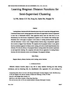
St. Olaf College Department of Mathematics, Statistics, and Computer Science Northfield, MN 55057 USA e-mail: [email protected] 2 Winona State University Department of Mathematics and Statistics Winona, WI 55987 email: [email protected] 3 James Madison University Department of Mathematics and Statistics Harrisonburg, VA 22807 email: [email protected] Abstract To assess environmental health of a stream, field, or other ecological object, characteristics of that object should be compared to a set of reference objects known to be healthy. Using streams as objects, we propose a k-nearest neighbors algorithm (Bates Prins and Smith, 2006) to find the appropriate set of reference streams to use as a comparison set for any given test stream. Previously, investigations of the k-nearest neighbors algorithm have utilized a variety of distance functions, the best of which has been the Interpolated Value Difference Metric (IVDM), proposed by Wilson and Martinez (1997). We propose two alternatives to the IVDM: Wilson and Martinez’s Windowed Value Difference Metric (WVDM) and the Density-Based Value Difference Metric (DBVDM) developed by Wojna (2005). We extend the WVDM and DBVDM to handle continuous response variables and compare these distance measures to the IVDM within the ecological k-nearest neighbors context. Additionally, we compare two existing attribute weighting schemes (Wojna 2005) when applied to the IVDM, WVDM, and DBVDM, and we propose a new attribute weighting method for use with these distance functions as well. In assessing environmental impairment, the WVDM and DBVDM were slight improvements over the IVDM. Attribute weighting also increased the effectiveness of the k-nearest neighbors algorithm in this ecological setting. ∗

This research was supported by NSF grant NSF-DMS 0552577 and was conducted during an 8-week summer research experience for undergraduates (REU).

EPUMD 4, 2010 No. 3

Distance Functions and Attribute Weighting

2

Key words and phrases: Nearest-neighbor, distance function, classification, mixedtype variables.

1

Introduction

When determining the health of ecological objects, test objects of unknown health status are compared to a set of reference objects, which are assumed to be healthy. In this application, we consider a set of n streams that are all assumed to be unimpaired. These streams form our set of reference streams. Using various biological metrics known to be correlated with stream health, the metric values of test streams, or streams of unknown impairment status, will be compared to the metric values of that test stream’s k nearest neighbors. Since ideal metric values vary based on a variety of factors, we seek to determine which k neighbors are most similar to the test stream. To find the neighbors, we use a distance function defined on pre-selected predictors. Very generally, the distance between any reference stream and test stream can be defined as: DIST (x, y) =

m X

dista (xa , ya )

(1)

a=1

where x and y are streams between which we desire to find the distance, a indicates the ath predictor, m is the number of predictors, and xa and ya are the values of predictor a for observations x and y respectively. In our application, we define x to be a test stream and y to be a reference stream, meaning that x is not included in the reference dataset, but y is. Then dista is defined as:  if predictor a is categorical   vdma (xa , ya ) C X dista (xa , ya ) = (2) |Pa,xa ,c − Pa,ya ,c |2 otherwise   c=1

where vdma is the Value Difference Metric (VDM) defined on predictor a (Wilson and Martinez [3]), c is an indicator for the output class, C is the total number of output classes, and Pa,xa ,c is the conditional probability that the output class is c given that predictor a has value x. In mathematical terms, Pa,xa ,c = P (c|xa ). Because predictors may be either categorical or continuous, a good distance function must allow for both. Spencer et al. [2] discuss the problem of scaling the possible contributions of continuous predictors to be equivalent to the possible contributions of categorical predictors. We analyze three different distance functions that incorporate both categorical and continuous predictors: the Interpolated Value Difference Metric (IVDM) (Wilson and Martinez [3]), the Windowed Value Difference Metric (WVDM) (Wilson and Martinez, [3]), and the Density-Based Value Difference Metric (DBVDM) (Wojna [5]). Though all these methods were originally developed to classify objects into categories (i.e. for use with categorical response variables), the IVDM was modified to handle continuous responses by Spencer et al. [2]. Because the biological metrics EPUMD 4, 2010 No. 3


3

we are considering are continuous, we have modified the WVDM and the DBVDM to handle continuous responses as well. In addition, we hypothesize that not all predictors are equally effective at determining stream similarity. We seek to incorporate predictor effectiveness into our distance functions by utilizing predictor weighting. We consider three weighting schemes for use with the proposed distance functions: Weights Optimizing Distance (Wojna [5] Algorithm 1), Weights Optimizing Classification Accuracy (Wojna [5] Algorithm 2), and Scaled Misclassification Ratio Weighting Method. When weighting is introduced, the distance is defined as: DISTweighted (x, y) =

m X

weighta · dista (xa , ya )

(3)

a=1

where weighta is the weight for the ath predictor and is assumed constant for all streams. In this paper, we compare the IVDM, WVDM, and the DBVDM, applying weights to each method and comparing the weighted methods with the unweighted. We also compare the effectiveness of the three different weighting schemes.

2

The Windowed Value Difference Metric (WVDM)

The WVDM was introduced by Wilson and Martinez [3] and functions similarly to the IVDM of those authors. However, instead of sampling values of Pa,x,c only at the midpoint of each of the predictor’s discretized ranges, the WVDM samples Pa,x,c at every value of predictor a that occurs in the reference dataset. The WVDM was originally proposed to handle classification problems i.e., problems with categorical responses. Here we extend the WVDM to continuous responses. To do this, we first discretize the response into C output classes. Let J = {1, 2, ..., n} represent the indices for the n objects in the reference dataset. The output class associated with the response R observed at observation p is defined as follows:  if Rp ≥max{Rj }, j ∈ J  C 1 if Rp ≤min{Rj }, j ∈ J discretize(Rp ) = (4)  b(Rp −minj∈J {Rj })/wc + 1 j ∈ J, otherwise, where w indicates the width of each output class. We define w = C1 | max{Rj }−min{Rj }|, where j ∈ J. After discretizing the response variable, the WVDM uses the general distance equations (1) and (2), or (3) instead of (1) if using weights. In using equation (2), we need to calculate Pa,xa ,c and Pa,ya ,c . To find these values, we first calculate Pa,xa ,c for each value, xa , of predictor a occurring in the reference dataset by considering the number of observations with values of predictor a that fall within a window centered at xa with width wa , defined as wa = 1s · | max(xaj ) − min(xaj )| where j ∈ J. A value for EPUMD 4, 2010 No. 3


4

0.7

0.7

s is chosen to determine window size, but the value of s is somewhat arbitrary and has been shown to have little bearing on results (Wilson and Martinez [3], Spencer et al. [2]). Then Pa,xa ,c is the proportion of observations in the window for xa that have output class C. Once the values of Pa,xa ,c are calculated for all values of xa occurring in the reference dataset, probabilities can be calculated for any value of xa , whether it occurs in the reference dataset or not. If xa occurs in the reference dataset, Pa,xa ,c is known based on the calculations performed in the previous step. If xa does not occur in the training set, choose x1 , x2 such that x1 , x2 are values of predictor a occurring in the reference dataset and x1 < xa < x2 . Then Pa,xa ,c is found by linear interpolation between Pa,x1 ,c and Pa,x2 ,c . For test values lying outside the range of reference values, the convention of Wilson and Martinez [3] was followed; values were interpolated toward zero.

0.4

0.5

0.6

Output Class 2 (c=2) Output Class 4 (c=4) Test Stream Reference Stream

0.0

0.1

0.2

0.3

Probability (Pa,xa,c)

0.4 0.3 0.0

0.1

0.2

Probability (Pa,xa,c)

0.5

0.6

Output Class 2 (c=2) Output Class 4 (c=4) Test Stream Reference Stream

1.5

2.0

2.5

3.0 Value of xa (area)

3.5

4.0

4.5

1.5

2.0

2.5

3.0

3.5

4.0

4.5

Value of xa (area)

Figure 1: Probability Profiles from WVDM (left) and DBVDM (right) methods Problems with the WVDM can arise if the reference dataset is too sparse [5]. Since the window width wa is fixed for each predictor, it may not capture enough observations to calculate accurate probabilities, and in other cases, the window may be too small to capture any observations. In this case, Na,x = 0, which causes problems since Na,x is the denominator of Pa,x,c . One solution to this problem is to use the DBVDM (Density-Based Value Difference Metric), which sets the window using a fixed number of observations rather than a fixed width. This method also allows us to calculate Pa,x,c the same way for all test values, whether their values fall within the reference set range or not.

EPUMD 4, 2010 No. 3


3

5

The Density-Based Value Difference Metric (DBVDM)

The DBVDM is an adaptation to the WVDM developed in [5]. The WVDM determines a constant width for the moving window; the number of observations that fall inside this window is variable. The DBVDM, however, has a constant number of observations in all windows, while the width of the windows is variable. Like the WVDM, the DBVDM samples Pa,xa ,c at every value of predictor a that occurs in the reference dataset. The DBVDM uses the general formula for a distance function (equations (2) and (1) or (3) if weighted). The DBVDM method was developed to handle the problems that could occur with the WVDM, namely that of sparse reference data. Including a fixed number of observations in every window addresses this issue. We have extended the DBVDM to handle a continuous response by using equation (4) to discretize the response into C output classes. We then calculate Pa,xa ,c for each predictor a in the reference dataset by considering each value xa of predictor a occurring in the reference data and selecting the nw observations with values of predictor a that are closest to xa . These nw observations form the window for the value xa . In the event of a tie between closest observations, we randomly select observations from the tied values. Pa,xa ,c is then defined as the proportion of observations in the window centered at xa with output class c. Figure 1 shows graphs of Pa,xa ,c for c = {1, 2, 3, 4, 5, 6} for the WVDM and DBVDM methods. Here, xa represents values of a predictor (catchment area in this example). The vertical lines represent values of catchment area for a test stream (x, dashed line) and a reference stream (y, dashed/dotted line). Here, xa = 2.172 and ya = 3.40. The WVDM distance is calculated by taking the sum of squared differences between Pa,xa ,c and Pa,ya ,c for each c, i.e. differences between probabilities associated with points of the same shape lying on different vertical lines. Because we calculate Pa,xa ,c at all the reference values rather than only s reference values as is done in the IVDM, we obtain a more accurate probability profile with the WVDM and DBVDM. Notice the discrete horizontal lines occurring in the DBVDM plot; this is due to the fact that Pa,xa ,c is always calculated with the same denominator (nw ), so there are only nw +1 possiblities for the value of Pa,xa ,c .

4

Attribute Weighting Schemes

We now discuss three approaches to determining the value of weighta , the weight for predictor a used in the distance function given in (3).

EPUMD 4, 2010 No. 3


4.1

6

Weights Optimizing Distance (Wojna Algorithm 1)

The first weighting method we tested on our data was the algorithm optimizing distance in Wojna [5]. This approach gives higher weights to predictors that put a large distance between two sites with different output classes. From our 87 streams, a random test sample (Stest ) of size 30 was selected, leaving 57 streams in a training set. The nearest neighbor of each stream x in the test set is found using all predictors. If the output class of x does not match the output class of x’s nearest neighbor (nearest(x)), x is included in the set misclass. Define dist(x, y) as the total distance between test stream x and reference stream y and define dista (x, y) as the distance between test stream x and reference stream y using only predictor a. We then define a global misclassification ratio M R and a predictor-specific misclassification ratio M R(a) as follows: X MR =

x∈misclass

X

x∈Stest

X

dist(x, nearest(x)) dist(x, nearest(x))

,

M R(a) =

dista (x, nearest(x))

x∈misclass

X

dista (x, nearest(x))

, (5)

x∈Stest

where nearest(x) is the same reference stream in the numerator and denominator of both M R and M R(a) and is found using all predictors. Then if M R(a) > M R, the weight for predictor a is additively increased by the value modif ier, initially defined to be 0.9. This entire process, beginning with random selection of Stest , is then repeated l times, multiplying modif ier by 0.9 each time. After running simulations with varying values of l, we followed Wojna’s convention and used l = 20; more iterations did not improve the results. The interested reader can refer to Wojna [5] for further details on this method.

4.2

Weights Optimizing Classification Accuracy (Wojna Algorithm 2)

Wojna [5] also proposes a weighting method that optimizes classification accuracy. This weighting scheme gives higher weights to predictors that define the nearest neighbor of a particular stream to be a stream of the same output class. The weight for each attribute is initialized to be 1. Like the previous method, this weighting scheme first selects a random set of 30 streams to be the test set (Stest ) and uses the remaining 57 streams as reference streams. Using the given distance function, for each of the 30 test streams (x), the method finds the nearest neighbor in the reference set with the same output class as the test stream (nearest(x)) and the nearest neighbor in the reference set with an output class different from the test stream (nearest(x)). The distances to these neighbors are calculated using all predictors. Next, the method calculates correct as the number of streams x ∈ Stest that are closer to nearest(x) than to nearest(x), using distances based on all predictors. Then correct(a) is similarly calculated, using EPUMD 4, 2010 No. 3


7

distances based only on predictor a (but still using the same streams for nearest(x) and nearest(x), found using all predictors). If correct(a) > correct, the weight for predictor a is additively increased by the value modif ier, initially defined to be 0.9. This entire process is repeated l times, multiplying modif ier by 0.9 each time. We again used l = 20 iterations.

4.3

Scaled Misclassification Ratio Weighting Method

In addition to the two methods created by Wojna, we tested a weighting method of our own design. The main criterion for measuring the effectiveness of predictor a was the misclassification ratio for that predictor i.e. M R(a), defined in (5). The steps for this algorithm are the same as those in the algorithm optimizing distance (Wojna Algorithm 1) until the weights are calculated. After finding the values of M R(a) and M R, predictor a is simply assigned a weight of MMR(a) . We hypothesized that R assigning weights directly related to M R(a) would improve the weighting scheme. The other weighting scheme simply increments the weight for predictor a if M R(a) > M R without accounting for the magnitude of the difference between M R(a) and M R. By assigning predictor a the weight MMR(a) , we hoped to better incorporate the magnitude R of the difference into the weighting system.

5

Data

Our analysis was based on the data used by Bates Prins and Smith [1]. This dataset consisted of n = 87 reference streams in the mid-Atlantic highlands region. For each stream, six different biological metrics (responses) were measured. These metrics include Ephemeroptera richness (EPHERICH), Plecoptera richness (PLECRICH), total taxa richness (TOTLRICH), tolerant taxa richness (TOLRRICH), proportional abundance of tolerant taxa of aquatic microinvertebrates (TOLRPIND), and proportional abundance of the three most common taxa (DOM3PIND). Predictors considered in our analysis included log-transformed catchment area (AREA), latitude (LAT), longitude (LON), total rapid bioassessment protocol habitat score (RBP), and Level III Ecoregion (ECO) as assigned by the EPA. All predictors are continuous except for ecoregion, which has 6 levels. Further details regarding the data can be found in Bates Prins and Smith [1]. All analysis was done in R Versions 2.9.0 and 2.4.1.

6

Methods of Comparison

Our comparison of the IVDM, WVDM, and DBVDM methods and our analysis of the effectiveness of attribute weighting was done using the leave-one-out approach described in Bates Prins and Smith [1]. Using the leave-one-out method and the EPUMD 4, 2010 No. 3


8

mean squared error of prediction (MSE), the best neighborhood size (k) along with the optimal subset of predictors was chosen. A low MSE indicated good choices of k and predictors. Each stream in our dataset in turn was treated as a test stream of unknown output class and unknown impairment status, and the k and predictor subset generating the lowest MSE were chosen. The distance function was then used to find the k nearest neighbors of the “test” stream. The response values of these neighbors were used to determine the scaled response value of the test stream, which determined the test stream’s impairment status as described in Bates Prins and Smith [1]; following their convention, a cutoff of α = 0.05 was used. Each of our “test” streams in actuality comes from our reference dataset, which is composed of streams known to be minimally impaired, so the impairment status for all the reference streams should be found to be not impaired. For each metric, classification accuracy (percentage of reference streams classified as not impaired) was measured; a classification rate of 100 indicates a good distance function. These two criteria (MSE and classification rate) served as a basis for our comparisons. We also experimented with different window widths for the WVDM and DBVDM, different numbers of input classes for the IVDM, and different numbers of output classes for all three distance functions. Following the convention of Wilson and Martinez [3, 4] and Spencer, Bates Prins, and Beckom [2], we used a heuristic approach in choosing values of s and C for the WVDM. Because ecoregion has 6 levels, we first set s = 6 and C = 6. After testing this case, we tried two smaller window widths (s = 8 and s = 12) and one larger window width (s = 4). We set C = 6 initally based on Wilson and Martinez’s tests [3], but also tried using different numbers of output classes by setting C = 3, C = 9, and C = 12. The same choices for C were used in the DBVDM. For the window size in the DBVDM, we originally set nw = 12, which corresponded to 13.7% of the reference dataset. This was based on Wojna’s choice of nw = 12 in proportion to the size of his datasets [5]. We also used a smaller window (nw = 8) and a larger window (nw = 16) in testing this method. We chose our “large-window” nw to correspond approximately to our “large-window” s, and our “small-window” nw to correspond to our “small-window” s. We note that 87/6 = 14.5 (so n/s is close to 16, our chosen value of nw ), and also that 87/12 = 7.25 (so n/s is close to 8, our chosen nw ). Because of this correspondence, we were able to make a fair comparison between weighting methods.

7

Results

In extending the WVDM and DBVDM to handle continuous response variables, we found that these methods are at least comparable to the IVDM, and in most cases, they perform better than the IVDM in terms of both MSE and classification rate, even without attribute weighting. In particular, the DBVDM performs well as measured by MSE, generating lower MSEs than the IVDM and WVDM for 5 of the 6 metrics. For the last metric (DOM3PIND), the WVDM generated a lower MSE than the IVDM, so EPUMD 4, 2010 No. 3


9

for all metrics, the IVDM is outperformed in terms of MSE. Table 1 gives the best MSE values for each distance function without weighting. MSE and classification rates for IVDM in Table 1 were taken from Spencer et al [2]; all WVDM and DBVDM measures are original work. In terms of weights, for all metrics, a weighted distance function was optimal in terms of MSE, with Wojna’s algorithm optimizing distance performing best for three metrics (EPHERICH, TOLRRICH, and DOM3PIND), Wojna’s algorithm optimizing classification accuracy performing best for two metrics (PLECRICH and TOLRPIND), and our scaled misclassification ratio weighting scheme performing best on one metric (TOTLRICH). For four of the six metrics, our scaled misclassification ratio scheme performed similarly to the best weighting scheme. In terms of classification accuracy, our scaled misclassification ratio weighting method performed best on 3 of the metrics (PLECRICH, TOTLRICH, and TOLRRICH), Wojna’s method optimizing classification accuracy performed best on one metric (DOM3PIND), and unweighted distance functions were optimal on the other two metrics, although the differences were small. Table 2 details the distance functions’ performance with weighting schemes. We were also interested in these distance functions’ ability to use both categorical and continuous predictors in determining distances. The inclusion of ecoregion, a categorical variable, as a predictor in our optimal predictor subsets is an indicator that these distance functions were somewhat successful at mixing the two types of attributes. In the unweighted methods, ecoregion was chosen as a predictor by at least two distance functions for 3 of the 6 metrics (EPHERICH, TOLRPIND, and DOM3PIND). For the weighing methods, ecoregion was frequently chosen when analyzing those three metrics as well. Ecoregion was never chosen as a predictor for any of the other three metrics. Ecoregion’s inclusion in the predictor set for half of the metrics indicates that these distance functions are somewhat successfully mixing continuous and categorical attributes.

8

Discussion

In our analysis of optimal distance functions and weighting methods, we found the WVDM to be a slight improvement over the IVDM, and we found the DBVDM to be substantially better than the IVDM in terms of MSE. Classification accuracy was not diminished when using the DBVDM. We believe the improvements over the IVDM are due to the fact that the WVDM and DBVDM calculate the values of Pa,xa ,c with more precision than does IVDM. The window of variable width in the DBVDM appears to be the reason for its good performance, since window size is the only difference between the DBVDM and the WVDM. Using the same number of observations in each window eliminates the problems of empty windows, windows with very few observations, and test sites with predictor values lying outside the predictor’s range in the reference dataset. The weighting methods also improved MSE, but there was no clear pattern as EPUMD 4, 2010 No. 3


10

Table 1: The minimum mean squared error (MSE) obtained by each method without attribute weighting. The MSE is listed along with the k, subset of predictors, s or nw , and C associated with that MSE. Also included is RATE, the percentage of times a reference stream was correctly classified as unimpaired. Low MSEs and high classification rates are desirable. The lowest MSE for each metric is in bold. A Xindicates the inclusion of a predictor in the nearest-neighbor distance calculation.

Method IVDM WVDM DBVDM






MSE 8.57 8.03 7.82

MSE 3.74 3.85 3.54

MSE 134.03 125.0 118.9

MSE 2.49 2.47 2.51

MSE 0.00614 0.00598 0.00580

MSE 0.0186 0.0167 0.0162

RATE 94 97 95

EPHERICH k AREA LAT LON 21 X 14 X X 18 X

RATE 98 94 95

PLECRICH k AREA LAT LON 11 X X 15 X X 14 X

RATE k 92 20 92 15 93 14

TOTLRICH AREA LAT LON X X X X X X

RATE 97 91 93

TOLRRICH k AREA LAT LON 25 X X 21 X 21 X

RATE 95 95 94

k 15 7 7

TOLRPIND AREA LAT LON X X X X X

k 18 20 11

DOM3PIND AREA LAT LON X X X X X

RATE 95 94 94

RBP

ECO X X X

Width C s=6 6 s=4 9 nw =16 9

RBP

ECO

Width C s=12 6 s=12 9 nw =12 9

RBP

ECO

Width C s=12 6 s=4 9 nw =12 6

RBP

ECO

Width C s=6 6 s=6 6 nw =16 3

RBP

ECO

X X

X X

Width C s=6 6 s=6 9 nw =16 9

RBP

ECO X X

X

X

Width C s=6 6 s=4 3 nw =16 9

EPUMD 4, 2010 No. 3


11

Table 2: The minimum mean squared error (MSE) obtained by each method using each weighting scheme. The classification rate associated with that MSE is also listed. The best MSE for each distance function within a metric is in bold. For each metric, the best overall MSE and classification rate are in boxes. EPHERICH Method IVDM WVDM DBVDM

MSE

Classification Rate

No Weights

Wojna 1

Wojna 2

Scaled MR

No Weights

Wojna 1

Wojna 2

Scaled MR

8.57 8.03 7.82

8.83 8.26 7.71

8.43 8.13 8.25

8.28 8.19 7.77

94 97 95

93 95 95

94 95 94

90 95 95

PLECRICH Method IVDM WVDM DBVDM

MSE

Classification Rate

No Weights

Wojna 1

Wojna 2

Scaled MR

No Weights

Wojna 1

Wojna 2

Scaled MR

3.74 3.85 3.54

3.54 3.80 3.56

3.79 3.84 3.51

3.72 3.81 3.58

98 94 95

94 94 95

93 94 94

98 94 98

TOTLRICH Method IVDM WVDM DBVDM

MSE

Classification Rate

No Weights

Wojna 1

Wojna 2

Scaled MR

No Weights

Wojna 1

Wojna 2

Scaled MR

134.0 125.0 118.9

122.7 126.6 120.2

123.1 123.3 119.0

123.2 124.7 116.9

92 92 93

93 93 94

92 91 92

92 93 95

TOLRRICH Method IVDM WVDM DBVDM

MSE

Classification Rate

No Weights

Wojna 1

Wojna 2

Scaled MR

No Weights

Wojna 1

Wojna 2

Scaled MR

2.49 2.47 2.51

2.51 2.47 2.43

2.49 2.47 2.51

2.50 2.47 2.45

97 91 93

90 91 92

94 91 93

97 91 94

TOLRPIND Method IVDM WVDM DBVDM

MSE

Classification Rate

No Weights

Wojna 1

Wojna 2

Scaled MR

No Weights

Wojna 1

Wojna 2

Scaled MR

0.00614 0.00598 0.00580

0.00591 0.00586 0.00592

0.00590 0.00590 0.00565

0.00597 0.00590 0.00593

95 95 94

92 93 94

94 94 92

93 92 94

EPUMD 4, 2010 No. 3


12

DOM3PIND Method IVDM WVDM DBVDM

MSE

Classification Rate

No Weights

Wojna 1

Wojna 2

Scaled MR

No Weights

Wojna 1

Wojna 2

Scaled MR

0.0186 0.0167 0.0162

0.0155 0.0166 0.0158

0.0163 0.0171 0.0160

0.0165 0.0166 0.0162

95 94 94

94 91 94

97 93 95

94 95 95

to when each weighting scheme would be optimal; the best weighting scheme appears to be dependent on the metric. The scaled misclassification ratio method performed best in terms of classification accuracy, while the other methods performed better in terms of MSE. Based on these experiments, we recommend the DBVDM with some choice of weighting scheme. All results incorporated variable selection by way of the forward selection process described in Bates Prins and Smith [1]. It can be argued that all predictors should be used in calculating distances to nearest neighbors (the calculation is faster and it makes use of all available information) but that the predictors should be weighted in terms of importance or accuracy. We ran all three distance functions with weights (all schemes) but without variable selection, and found that eliminating variable selection (even when using attribute weighting) noticeably increased MSE. We hypothesize that variable selection is still worthwhile, even when using attribute weighting, because the weighting methods do not always give higher weights to those predictors that are selected in variable selection. This is due to the fact that variable selection uses MSE as its criteria for important predictors, while the attribute weighting does not. Applying both weighting and selection gives the best overall results. One question we came across was that of how to calculate Pa,xa ,c for values lying outside the range of reference values in the WVDM. Recall that w indicates window width and J indicates the reference set. Our analysis simply calculated Pa,xa ,c = 0 when xa = max xaj + w2 and when xa = min xaj − w2 , j ∈ J. This means that if our test value was in the window of max xaj or min xaj , interpolation was performed as usual. If the test value was so extreme that it fell outside that window, probabilities for all output classes were calculated as 0. Instead of using this approach, another option is to set Pa,xa ,c for any xa < min xaj to be equal to Pa,min xaj ,c and similarly, to set Pa,xa ,c for any xa > max xaj to Pa,max xaj ,c . This method seemed to make more sense because intuitively, it seemed that every test stream should have a nonzero probability of being in at least one output class. Due to the lack of interpolation and the method of determining observations in the windows in the DBVDM, this alternative proposal is actually occurring in that method. We tested the WVDM using this alternative approach for outlying test values and found that it had little bearing on the results, possibly because we only tested a small number of outlying values. Future research may include investigating better ways of handling outlying test values. EPUMD 4, 2010 No. 3


13

Though we recommend the DBVDM with a weighting scheme for use, these methods are not flawless. Both the DBVDM and the WVDM are computationally more intensive than the IVDM, so running these methods on large datasets may take more time than desired. Attribute weighting also adds more time in computation. As in the IVDM, the choice of window size and output class size is somewhat subjective. In our analysis, using different window sizes or output class sizes changed some MSE values by a small amount, but in general, the choice of s, nw , or C had little bearing on results (Spencer et al [2]). The choices of the values for s, nw , and C did not follow any clear pattern, and our optimal results for these values were based on experimentation. Finally, more research is needed as to what values of l (number of iterations) and |Stest | (test set size) are optimal for a small dataset like ours. There is also some subjectivity in the choice of initial value of modif ier in Wojna’s algorithms: setting its initial value to 0.9 and its subsequent values to powers of 0.9 generates attribute weights that are sums of the geometric series 1 + 0.9 + 0.92 + ... + 0.9r where r is the number of times the weight is increased, and these weights have a maximum value of 10. Different values of modif ier will generate different values for the maximum attribute weight. Choosing a different value for modif ier would not affect results, but it is somewhat arbitrary. One solution to this problem would be to use our scaled misclassification ratio scheme that uses the actual misclassification ratios rather than an arbitrary modifier to determine predictor weights. Overall, the DBVDM and weighting schemes were improvements over the IVDM, providing good distance functions that utilize categorical and continuous predictors and have the flexibility to be used in many settings.

References [1] S. C. Bates Prins and E. P. Smith, Using biological metrics to score and evaluate sites: A nearest-neighbor reference condition approach, Freshwater Biology 50 (2006), 635–639. [2] M. S. Spencer, S. C. Bates Prins, S.C. and M. S. Beckom, Heterogeneous distance measures and nearest-neighbor classification in an ecological setting, preprint. [3] D. R. Wilson and T. R. Martinez, Improved heterogeneous distance functions, Journal of Artificial Intelligence Research 6 (1997), 1–34. [4] D. R. Wilson and T. R. Martinez, An integrated instance-based learning algorithm, Computer Intelligence 16 (1) (2000), 1–28. [5] A. Wojna, Analogy-based reasoning in classifier construction, Lecture Notes in Computer Science 3700 (2005), 277–374.

EPUMD 4, 2010 No. 3