wind characteristics (wind intensity and direction), as well as turbines' ... [m]. D. Wind turbine rotor diameter. [m] v. Velocity behind the rotor. [m/s] v0 ... the effects of rotating blades are the dominant factors (helical ... of the wind turbine wake is shown. In the same figure, typical downstream air velocity .... 14° 45' 02.69882''.
International Journal of Applied Engineering Research ISSN 0973-4562 Volume 12, Number 24 (2017) pp. 16068-16076 © Research India Publications. http://www.ripublication.com
Wind Turbine Wake Mathematical Models Validation by Means of Wind Field Data 1
Sebastian Brusca, 2Fabio Famoso, 3Antonio Galvagno, 4Rosario Lanzafame, 5Stefano Mauro and 6Michele Messina
1,2,3,4,5
PhD, Department of Civil Engineering and Architecture, University of Catania, Viale A. Doria 6, Catania-95125, Italy. 2
Orcid: 0000-0003-3880-0292 & Scopus ID: 56029382400
Abstract The present paper deals with a study of wind turbine performance taking into account wind turbine interaction in wind farms. In more details, a wake mathematical model, based on Jensen/Katic theory, was implemented and used to evaluate velocity deficit at the downstream turbine. In order to test and verify wake mathematical model implementation, wind farm real data were used. Turbines in pairs data were extracted from wind farm monitoring system and were elaborated to collect wind characteristics (wind intensity and direction), as well as turbines’ powers and wind intensity at the turbines’ nacelles. On the basis of the presented results, the implemented mathematical model is able to correctly estimate velocity deficit while errors on downstream power were lower than 10 % in all cases. Therefore, the model is validated. Keywords: Wind Turbine; Wake; Mathematical Modelling; Wind Field; Optimal WT Placement.
new renewable, and also environmental and emissions regulations and standards [1, 2]. In the last decade energy demand was strongly increased despite of economic crisis and energy saving actions [3-5]. According to International Energy Agency [6] scenario, the recent government commitments are implemented in a cautious manner (IEA – New Policies Scenario), primary energy demand increased by one-third between 2010 and 2035, with 90 % of the growth in non-OECD economies. Taking into account these factors and environmental constrains, renewable energy sources will play an important role in the near future energy scenario and among them wind energy plays will play an important role in the future [7-8-9]. In order to reduce terrain occupation and visual impact of wind turbines, they are generally clustered in wind farms [10]. This implies wind turbine interaction. Wind turbine interaction may have severe implications in the downstream turbines, such as: 1.
Nomenclature Variable OECD x D v v0 v1 r0 r a CT rw α z z0 vT zref vref
Description Organisation for Economic Cooperation and Development Distance from the rotor Wind turbine rotor diameter Velocity behind the rotor Undisturbed velocity of the flow investing the rotor Flow velocity downstream the rotor Rotor radius Downstream wake radius Axial induction coefficient Turbine thrust coefficient Wake radius Decay coefficient Height of turbine hub Roughness Air velocity at turbine height Reference height air velocity at reference height zref
UOM -
2.
[m] [m] [m/s] [m/s]
Because of stream-wise velocity deficit caused by the wake, the downstream turbines generates less power [11]; Because of high turbulence levels in the wake, the downstream turbines experiences an increase in fatigue loads [12].
Turbine wake characteristics and development depends on many factors: 1. 2. 3.
[m/s] [m] [m] [m] [m] [m] [m/s] [m/s] [m/s]
Wind conditions; Site topology; Upstream turbine operating conditions.
To reduce the impact of the wake in a wind farm, wind farm designers use wake models and commercial software. Several times these models need to be validated to ensure that they are able to reproduce and, eventually, to know the uncertainty margin. Wind turbine wake models’ validation can be done using real data: a. b.
Wind tunnel data Wind farm data
INTRODUCTION
The main problems with using wind tunnel data are the scaling effect and wind tunnel wall interference of turbine models (blockage effect).
Future energy growth is affected by many factors, mainly such as: economic growth, population growth, energy prices and fuel availability, technologies that improve efficiency and develop
The benefit of using measurements from a wind farm is that the wake models are tested with non-controlled real-life conditions.
16068
International Journal of Applied Engineering Research ISSN 0973-4562 Volume 12, Number 24 (2017) pp. 16068-16076 © Research India Publications. http://www.ripublication.com The present paper deals with a study of wind turbine performance taking into account wind turbine interaction in wind farms. In more details, a wake mathematical model, based on Jensen/Katic theory, was implemented and used to evaluate velocity deficit at the downstream turbine. In order to test and verify wake mathematical model implementation, wind farm real data were used.
uniform deficits of pressure and axial velocity, as well. These deficits are related to axial thrust, azimuthal component of the velocity (related to turbine torque), as well as vortex sheets (related to circulation along the blades variation) that are shed from the trailing edge and roll up in a short downstream distance, forming tip vortices with helical trajectories [16].
WAKE MATHEMATICAL MODEL
The Jensen wake model [17] is popular as an engineering wind turbine wake model for the quantification of the reduction of the wind speed downstream a wind turbine. This is because it was formulated in the early 1980s when only a few wake models were available and is simple, very fast and easy to implement. It is also the base of the Park model [18] that was developed for wind farm calculations for the Wind Atlas Analysis and Application Program [19], which is widely used for the estimation of wind resources. The simplicity of this model derived the assumption that the wake expands linearly downstream the turbine with a velocity loss depending only on the distance behind the rotor. In order to describe the wake produced by a turbine this model is based on the following simplifying assumptions:
A wake is the region of recirculating flow immediately behind a moving or stationary blunt body, caused by viscosity, which may be accompanied by flow separation and turbulence. An air velocity deficit is registered in the wake. The wake of a wind turbine can be classified based on the distance from the turbine rotor: the near-wake (immediately behind the rotor) in which the effects of rotating blades are the dominant factors (helical tip vortex, high velocity deficit, etc.); the far-wake (at a distant behind the rotor disk) in which the geometric and aerodynamic characteristics of the turbine blades are less important. According to Schepers [13], Sedaghatizadeh et al [14], and Jimenez et al [15], the distance from the rotor to turbine diameter ratio discriminates near-wake from far-wake as follows: 𝑥 NEAR-WAKE 0 ≤ ≤5 𝐷 𝑥 FAR-WAKE >5 𝐷 In Fig. 1 a schematic representation of the wind turbine wake is shown. In the same figure, typical downstream air velocity deficit is indicated qualitatively.
In order to evaluate velocity deficit related to turbine wake, a mathematical model should be used.
Considering an air flow approaching a wind turbine, its velocity decreases while the pressure increases. Crossing the turbine rotor, a sudden decrease in pressure occurs. Therefore, in the region immediately downstream of the rotor, there are non-
The diameter of the wake right behind the turbine is assumed to be equal of the turbine’s diameter itself; The velocity profile inside the wake is considered ideal, constant along the ray; The wake expands linearly with a slope equal to the decay coefficient; The aerodynamic characteristics of the turbine are considered only through the thrust coefficient. The variations of pitch angle have to be modelled; The turbulence effects in the wake and in the wingtip vortices are not considered.
FAR-WAKE
NEAR-WAKE FREE STREAM
mixing zone VELOCITY DEFICIT
Figure 1. Wind turbine wake schematic representation with air velocity deficit
16069
International Journal of Applied Engineering Research ISSN 0973-4562 Volume 12, Number 24 (2017) pp. 16068-16076 © Research India Publications. http://www.ripublication.com This model was basically developed by applying the Momentum Conservation Principle around a control volume of the turbine wake. According to the symbols in Fig. 2, Eq. 1 describes this principle for a wind turbine: 𝜋𝑟02 𝑣 + 𝜋(𝑟 2 − 𝑟02 )𝑣0 = 𝜋𝑟 2 𝑣1
(1)
where: v is the velocity just behind the rotor; v0 is the undisturbed velocity of the flow investing the rotor; v1 is the flow velocity downstream the rotor; r0 and r are respectively the rotor radius and the downstream wake radius. Applying the Betz theory, it is possible to calculate the velocity just behind the rotor as a function of v0 thanks to Eq. 2. 𝑣 = (1 − 2𝑎)𝑣0
(2)
where a represents the axial induction coefficient that depends on the geometry of the rotor. In the original Jensen estimation, this coefficient was set equal to 1/3, but for a more accurate estimation it may be calculated using Eq. 3. (1 − √1 − 𝐶𝑇 ) (3) 2 where CT represents the turbine thrust coefficient. Finally, according to the assumption cited before about the linear expansion of the wake, its radius rw is calculated by Eq. 4. 𝑎=
𝑟𝑊 = 𝑟0 (1 + 2𝛼𝑥)
(4)
where x is the downstream distance from the turbine rotor and α is the decay coefficient. Fig. 2 shows the wake scheme according to the Jensen model with the velocity loss produced downstream the turbine. The decay coefficient allows to study the wake because it describes its extent at varying the distance from the rotor. It may be calculated by an empirical relation expressed in Eq. 5. 𝛼=
0,5 𝑧 ln( ) 𝑧0
(5)
where z is the height of the turbine hub and z0 is the roughness of the terrain. Substituting Eq. 2 and Eq. 3 in Eq. 1, it is possible to determinate the distribution of the velocity inside the wake area. Finally, this velocity v1 is expressed by Eq. 6. 𝑣1 = 𝑣0 [1 −
(a)
1 − √1 − 𝐶𝑇 ] (1 + 2𝛼𝑥)2
(6)
Figure 2. Wake evolution according Jensen theory From Eq. 6 it is possible to notice that the velocity distribution is function of CT, α, and x. Moreover, the velocity profile is constant along the radius r, with a typical “hat-shaped”. The estimation of the wake is not accurate close to the turbine rotor. Therefore the Eq. 6 is used only in the region 3÷8D, typical of the far-wake. Thanks to the simplifying assumptions Jensen’s model is one of the most used especially because of it computational fast responds. MATERIALS AND METHODS In order to test the mathematical model for wind turbine wake behaviour simulation, a real-life test case was considered. Actual data from a real wind farm were used. The case study is a large wind farm composed by 30 wind turbines and 3 anemometric towers. The wind farm is located in the south part of Italy in the rural area of Vizzini’s municipality (see Fig. 3a) and occupies an area of about 30 km2 at about 650 m above the sea level. The wind farm layout is shown in Fig. 3b, where red markers indicate the anemometer towers, while green ones the wind turbines. Fig. 3c shows a photograph of Vizzini’s wind farm, while in Table 1 and 2 anemometer towers and wind turbines coordinates and levels are reported.
(b)
(c)
Figure 3. Test case wind farm: (a) Location; (b) Wind turbines positions; (c) Wind farm photograph.
16070
International Journal of Applied Engineering Research ISSN 0973-4562 Volume 12, Number 24 (2017) pp. 16068-16076 © Research India Publications. http://www.ripublication.com Table 1. Anemometer towers localization and level Tower Code
Coordinates
Elevation
Nord
Est
[m] above sea-level
VIZ2
37° 13' 04.46384''
14° 44' 03.65126''
663.16
VIZ4
37° 14' 15.92171''
14° 44' 49.65503''
569.54
VIZ7
37° 13' 05.49844''
14° 42' 43.96433''
674.50
Table 2. Wind turbines localization and level Turbine Code
Coordinates
Elevation
Nord
Est
[m] above sea-level
VZ01
37° 12' 19.35171''
14° 44' 04.60503''
657.164
VZ02
37° 12' 24.14338''
14° 44' 02.60607''
668.051
VZ04
37° 12' 22.61844''
14° 44' 29.62433''
639.503
VZ05
37° 12' 26.78497''
14° 44' 33.31248''
638.436
VZ06
37° 12' 32.10942''
14° 44' 10.13667''
651.096
VZ07
37° 12' 38.96887''
14° 44' 03.06278''
650.205
VZ08
37° 12' 43.82043''
14° 44' 03.05817''
645.020
VZ09
37° 12' 48.61134''
14° 44' 01.29071''
641.214
VZ10
37° 12' 54.41851''
14° 44' 01.52223''
637.516
VZ11
37° 12' 58.99871''
14° 43' 59.38835''
644.928
VZ12
37° 13' 03.94462''
14° 44' 03.93243''
675.102
VZ13
37° 13' 08.31552''
14° 44' 09.17639''
662.904
VZ14
37° 13' 12.14585''
14° 44' 12.27781''
667.742
VZ15
37° 13' 16.47742''
14° 44' 14.40300''
656.959
VZ16
37° 13' 21.52066''
14° 44' 13.93384''
644.949
VZ17
37° 13' 25.67783''
14° 44' 17.20756''
640.757
VZ18
37° 13' 30.25997''
14° 44' 19.45528''
620.996
VZ19
37° 13' 35.10831''
14° 44' 19.50793''
605.165
VZ21
37° 13' 41.35184''
14° 44' 26.71442''
568.991
VZ22
37° 13' 51.95403''
14° 44' 32.16972''
603.211
VZ23
37° 13' 56.80502''
14° 44' 31.61148''
600.681
VZ25
37° 14' 12.76301''
14° 44' 49.15755''
580.388
VZ29
37° 14' 49.55258''
14° 45' 02.69882''
630.389
VZ30
37° 14' 55.24006''
14° 45' 09.78788''
641.755
VZ31
37° 15' 02.21863''
14° 45' 15.20036''
681.935
VZ32
37° 15' 08.13734''
14° 45' 20.87735''
651.215
VZ33
37° 12' 47.84338''
14° 42' 51.98149''
648.073
VZ34
37° 12' 52.46137''
14° 42' 48.71390''
671.004
VZ35
37° 12' 57.44880''
14° 42' 46.69092''
669.733
VZ36
37° 13' 02.19804''
14° 42' 44.01825''
680.063
As far as the site anemometric characteristics it is concerned, Fig. 4 shows the wind rose and the probability density function of the site at 30 m of one anemometric tower.
16071
International Journal of Applied Engineering Research ISSN 0973-4562 Volume 12, Number 24 (2017) pp. 16068-16076 © Research India Publications. http://www.ripublication.com N
0.16
1600 1400
0.14 1200
NE
1000
0.12 800
Probability density function [-]
600 400 200 W
E
0
0.1
0.08
0.06
0.04
0.02 SE NW
0 0
5
10
15
20
25
30
35
Wind velocity [m/s]
S
(a)
(b) Figure 4. Vizzini’s site anemometric characteristics.
All the Vizzini’s wind farm installed turbines are Vestas V52 upwind type turbines with a rated power of 850 kW. The main turbine characteristics are reported in Table 3, while in Fig. 4 and Fig. 5 turbine power curve (see Fig. 4), turbine power coefficient (see Fig. 5a) and turbine thrust coefficient (see Fig. 5b) are reported. A photograph of one of the installed turbine is shown in Fig. 6.
900
800
700
Turbine Power [kW]
600
Table 3. Wind turbine main characteristics Description Vendor
Value Vestas
Type
400
300
200
V52
Rated power
500
100
850 kW
0 0
5
10
15
20
25
30
Wind Speed [m/s]
Rotor diameter Grid connection
52 m 50/60 Hz
Turbine speed @ rated power
26 r/min
Hub height
49 m
Maximum blade width Blade width for 90% radius
2.30 m 0.4 m
0.5
1
0.45
0.9
0.4
0.8
0.35
0.7
Thrust Coefficient [-]
Power Coefficient [-]
Figure 4. Vestas V52 wind turbine power curve
0.3
0.25
0.2
0.6
0.5
0.4
0.15
0.3
0.1
0.2
0.05
0.1
0
0 0
5
10
15
20
25
0
30
5
10
15
Wind Speed [m/s]
Wind Speed [m/s]
(a)
(b)
Figure 5. Vestas V52 wind turbine: (a) power coefficient; (b) thrust coefficient
16072
20
25
30
International Journal of Applied Engineering Research ISSN 0973-4562 Volume 12, Number 24 (2017) pp. 16068-16076 © Research India Publications. http://www.ripublication.com Three case studies are analyzed as reported in Table 4. Table 4. Case studies main data Description
Wind direction [deg]
Turbine distance [m]
Case 1
VZ36 to VZ35
155
161.61
Case 2
VZ13 to VZ14
32.92
140.68
Case 3
VZ11 to VZ12
212.92
189.21
For each turbine and for all cases wind velocity deficit and wake radii, as well as turbine powers were evaluated. Moreover, turbine levels were taken into account. Figure 6. Vestas V52 wind turbine RESULTS AND DISCUSSION Data of turbines in pairs were extracted from wind farm monitoring system and data elaborated to collect wind characteristics (wind intensity and direction), as well as turbines’ powers and wind intensity at the turbines’ nacelles.
As far as the mathematical modelling it is concerned, a real data validation was carried out comparing calculated and experimental data. In Fig. 7, 8 and 9 calculated power versus real power for all analysed cases are shown. As defined earlier, couples of turbines were isolated in the wind farm data and power, wind intensity and direction were extracted from plant monitoring database. For each couple one turbine is in the wake of the other and vice versa. It is possible to observe that all the points in the graph lay on the straight forty-five degrees. Analysing the average relative errors, for all considered cases the error is always lower than 5 %. This confirms that the implemented model is validated.
From wind measurement towers, undisturbed wind intensities and directions are extracted for six turbines in pairs. Wind velocities were reported at turbine nacelle heights using Eq. 7. 𝑧 𝑙𝑛 ( ) 𝑧0 𝑣𝑇 = 𝑣𝑟𝑒𝑓 𝑧𝑟𝑒𝑓 𝑙𝑛 ( ) 𝑧𝑜
(7)
where vT is the air velocity at turbine height, vref is air velocity at reference height zref, z is the turbine height, z0 is the terrain roughness.
Moreover, real power data, calculated power, as well as manufacturer turbine power curve were compared (see Fig. 10) in all considered cases. It is well evident the good agreement between the data. This confirms the validity of the implemented method.
VZ35 Power in VZ36 wake
VZ36 Power in VZ35 wake
1000
900
900
800
800
700
Calculated Power [kW]
Calculated Power [kW]
700 600 500 400
600
500
400
300
300 200
200
100
100 0
0 0
100
200
300
400
500
600
700
800
900
0
Experimental Power [kW]
100
200
300
400
500
600
Experimental Power [kW]
(a)
(b)
Figure 7. CASE 1: calculated power versus experimental power of VZ35 and VZ36.
16073
700
800
900
International Journal of Applied Engineering Research ISSN 0973-4562 Volume 12, Number 24 (2017) pp. 16068-16076 © Research India Publications. http://www.ripublication.com VZ12 Power in VZ11 wake 1000
900
900
800
800
700
700
CAlculated Power [kW]
Calculated Power [kW]
VZ11 Power in VZ12 wake 1000
600 500 400
600 500 400
300
300
200
200
100
100
0
0 0
100
200
300
400
500
600
700
800
900
0
100
200
300
Experimental Power [kW]Titolo asse
400
500
600
700
800
900
Experimental Power [kW]
(a)
(b)
Figure 8. CASE 2: calculated power versus experimental power for VZ11 and VZ12.
VZ13 Power in VZ14 wake
VZ14 Power in VZ13 wake
1000
900
900
800
800
700
Calculated Power [kW]
600 500 400 300
600
500
400
300
200
200
100
100 0 0
100
200
300
400
500
600
700
800
900
0
Experimental Power [kW]
0
100
200
300
400
500
600
700
Experimental Power [kW]
(a)
(b)
Figure 9. CASE 3: Calculated power versus experimental power for VZ13 and VZ14.
VZ35 Power in VZ36 wake 1000 900 800 700
Power [kW]
Calculated Power [kW]
700
600 500 400 300 200 100 0 0
5
10
15
20
Wind velocity [m/s] Power curve
EXP
(a)
16074
CALC
25
30
800
900
International Journal of Applied Engineering Research ISSN 0973-4562 Volume 12, Number 24 (2017) pp. 16068-16076 © Research India Publications. http://www.ripublication.com VZ12 Power in VZ11 wake 1000 900 800
Power [kW]
700 600 500 400 300 200 100 0 0
5
10
15
20
25
30
20
25
30
Wind velocity [m/s] Power curve
EXP
CALC
(b) VZ14 Power in VZ13 wake 900 800 700
Power [kW]
600 500 400 300 200 100 0 0
5
10
15
Wind velocity [m/s] Power curve
EXP
CALC
(c) Figure 10. Manufacturer power curve, real and calculated power as a function of wind velocity: (a) CASE 1; (b) CASE 2; (c) CASE 3. household energy demands” Applied Energy, 97, pp. 723-733.
CONCLUSIONS In the present paper, a study on the wind turbine wakes is presented. A Jensen/Katic based wake mathematical model was implemented. Real data were used to test the model. From a wind farm monitoring system database, real power as well as wind intensity and direction were extracted and elaborated. Using the model, wake radii and velocity deficits were calculated and the calculated powers were determined for couples of turbines. The results were compared with real data and relative errors were calculated. On the basis of the results it is possible to state that the implemented model is validated (average relative error lower than 5 % in almost all considered cases). REFERENCES [1]
Air quality in Europe -2013 report, EEA report n. 9/2013 ISSN 1725-9177, doi:10.2800/92843.
[2]
Directive 2009/28/EC, 2009, “on the promotion of the use of energy from renewable sources”, Official Journal of the European Union.
[3]
Barbieri, E.S., Spina, P.R., Venturini, M., 2012, “ Analysis of innovative micro-CHP systems to meet
[4]
Yu, S., Wei, Y.M., Wang, K., 2012, “China’s primary energy demands in 2020: Predictions from an MPSORBF estimation model” Energy Conversion and Management, 61, pp. 59-66.
[5]
Puksec, T., Vad Mathiesen, B., Duic, N., 2011, “Long term energy demand projections for croatian transport sector” Proceedings of the 24th International Conference on Efficiency, Cost, Optimization, Simulation and Environmental Impact of Energy Systems, ECOS 2011, pp. 2576-2587.
[6]
International Energy Agency, 2011, “World Energy Outlook 2011” Soregraph, ISBN: 9789264124134.
[7]
Bartolini, N., Scappaticci, L., Garinei, A., Becchetti, M., Terzi, L., 2016, “Analyising wind turbine state dynamics for fault diagnosis”, Diagnostyka, 17(4), pp. 19-25.
[8]
Mauro, S., Brusca, S., Lanzafame, R., Famoso, F., Galvagno, A., Messina, M., 2017, “Small-Scale OpenCircuit Wind Tunnel: Design Criteria, Construction and Calibration” International Journal of Applied Engineering Research, 12(23), pp. 13649-13662.
[9]
Brusca, S., Lanzafame, R., 2003, “Analysis of syngas fed gas turbine performance depending on ambient
16075
International Journal of Applied Engineering Research ISSN 0973-4562 Volume 12, Number 24 (2017) pp. 16068-16076 © Research India Publications. http://www.ripublication.com conditions” American Society of Mechanical Engineers, International Gas Turbine Institute, Turbo Expo IGTI, pp. 943-948. [10]
Seim, F., Gravadahl, A.R., Adaramola, M.S., 2017, “Validation of kinematic wind turbine wake models in complex terrain using actual windfarm production data.” Energy, 123, pp. 742-753.
[11]
Yuan, W., Tian, W., Ozbay, A., Hu, H., 2014, “An experimental study on the effects f relative rotation direction on the wake interferences among tandem wind turbines” Science China: Physics, Mechanics and Astronomy, 57(5), pp. 935-949.
[12]
Chamorro, L.P., Arndt, R.E.A., Sotiropoulos, F., 2012, “Reynolds number dependence of turbulence statistics in the wake of wind turbines” Wind Energy, 15(5), pp. 733-742.
[13]
Schepers, J.G., 2003, “ENDOW: Validation and Improvement of ECN's Wake Model, EU 5th Framework Project ’Efficient Development of Offshore WindFarms’, (ENDOW),” Technical report.
[14]
Sedaghatizadeh, N., Arjomandi, M., Kelso, R., Cazzolato, B., Ghayesh, M. H., 2018, “Modelling of wind turbine wake using large eddy simulation.” Renewable Energy, 115, pp. 1166-1176.
[15]
Jimenez, A., Crespo, A., Migoya, E., Garcia, J., 2008, “Large-eddy simulation of spectral coherence in a wind turbine wake” Environmental Research Letters, 3, 1-9.
[16]
Crespo, A., Hernàndez, J., Frandsen, S., 1999, “Survey of Modelling Methods for Wind Turbine Wakes and Wind Farms.” Wind Energy, 2, pp. 1-24.
[17]
Jensen, N. O., 1983, “A note on wind generator interaction” Technical Report Risoe-M-2411(EN), Risoe-M-2411(EN), Risø National Laboratory, Roskilde.
[18]
Katic, I., Højstrup, J., Jensen, N.O., 2986, “A simple model for cluster efficiency.” Proceedings of the European Wind Energy Association Conference & Exhibition, pp. 407–410.
[19]
Mortensen, N.G., Heathfield, D.N., Myllerup, L., Landberg, L., Rathmann, O., 2007, “Getting started with WAsP 9” Technical Report Risø-I-2571(EN), Risø National Laboratory, Roskilde.
16076