Wireless Jamming Localization by Exploiting. Nodes' Hearing Ranges. Zhenhua
Liu1, Hongbo Liu2, Wenyuan Xu1, Yingying Chen2⋆. 1 Dept. of CSE, ...
Wireless Jamming Localization by Exploiting Nodes’ Hearing Ranges Zhenhua Liu1 , Hongbo Liu2 , Wenyuan Xu1 , Yingying Chen2? 1
2
Dept. of CSE, University of South Carolina {liuz,wyxu}@cse.sc.edu Dept. of ECE, Stevens Institute of Technology {hliu3,yingying.chen}@stevens.edu
Abstract. Jamming attacks are especially harmful when ensuring the dependability of wireless communication. Finding the position of a jammer will enable the network to actively exploit a wide range of defense strategies. Thus, in this paper, we focus on developing mechanisms to localize a jammer. We first conduct jamming effect analysis to examine how a hearing range, e.g., the area from which a node can successfully receive and decode the packet, alters with the jammer’s location and transmission power. Then, we show that the affected hearing range can be estimated purely by examining the network topology changes caused by jamming attacks. As such, we solve the jammer location estimation by constructing a least-squares problem, which exploits the changes of the hearing ranges. Compared with our previous iterativesearch-based virtual force algorithm, our proposed hearing-range-based algorithm exhibits lower computational cost (i.e., one-step instead of iterative searches) and higher localization accuracy.
1
Introduction
The rapid advancement of wireless technologies has enabled a broad class of new applications utilizing wireless networks, such as patient tracking and monitoring via sensors, traffic monitoring through vehicular ad hoc networks, and emergency rescue and recovery based on the availability of wireless signals. To ensure the successful deployment of these pervasive applications, the dependability of the underneath wireless communication becomes utmost important. One threat that is especially harmful is jamming attacks. The broadcast-based communication combined with the increasingly flexible programming interference of commodity devices makes launching jamming attacks with little effort. For instance, an adversary can easily purchase a commodity device and reprogram it to introduce packet collisions that force repeated backoff of other legitimate users and thus, disrupt network communications. To ensure the dependability of wireless communication, much work has been done to detect and defend against jamming attacks. In terms of detection, singlestatistics-based [13] and consistent-check-based algorithms [15] have been proposed. The existing countermeasures for coping with jamming include two types: ?
The work was supported by National Science Foundation Grants CNS-0845671 and CNS-0954020.
the proactive conventional physical-layer techniques that provide resilience to interference by employing advanced transceivers [10], e.g., frequency hopping, and the reactive non-physical-layer strategies that defend against jamming leveraging MAC or network layer mechanisms, e.g., adaptive error correcting codes [6], channel adaption [14], spatial relocation [5], or constructing wormholes [2] Few studies have been done in identifying the physical location of a jammer. However, localizing a jammer is an important task, which not only allows the network to actively exploit a wide range of defense strategies but also provides important information for network operations in various layers. For instance, a routing protocol can choose a route that does not traverse the jammed region to avoid wasting resources caused by failed packet deliveries. Alternatively, once a jammer’s location is identified, one can eliminate the jammer from the network by neutralizing it. In light of the benefits, in this paper, we address the problem of localizing a jammer. Although there have been active research in the area of localizing a wireless device [1, 3, 12], most of those localization schemes are inapplicable to jamming scenarios. For instance, many localization schemes require the wireless device to be equipped with specialized hardware [9, 12], e.g., ultrasound or infrared, or utilize signals transmitted from wireless devices to perform localization. Unfortunately, the jammer will not cooperate and the jamming signal is usually embedded in the legal signal and thus, is hard to extract, making the signalbased and special-hardware-based approaches inapplicable. Recent work [4, 7] on jamming localization algorithms is iterative-searchbased. Without presenting performance evaluation, Pelechrinis et al. [7] proposed to localize the jamming by measuring packet delivery rate (PDR) and performing gradient descent search. Liu et al. [4] utilized the network topology changes caused by jamming attacks and estimated the jammer’s position by introducing the concept of virtual forces. The virtual forces are derived from the node states and can guide the estimated location of the jammer towards its true position iteratively. In this paper, we proposed a hearing-range-based localization scheme that also exploits the network topology changes caused by jamming attacks. In particular, to quantify the network topology changes, we introduced the concept of a node’s hearing range, an area from which a node can successfully receive and decode the packet. We have discovered that a jammer may reduce the size of a node’s hearing range, and the level of changes is determined by the relative location of the jammer and its jamming intensity. Therefore, instead of searching for the jammer’s position iteratively, we can utilize the hearing range to localize the jammer in one round, which significantly reduces the computational cost yet achieves better localization performance than prior work [4]. We organize the remainder of the paper as follows: we specify our jamming attack model and provide an analysis on jamming effects by introducing the concept of the hearing range in Section 2. Then, we present our hearing-rangebased algorithm in Section 3. In Section 4, we conduct simulation evaluation and present the performance results. Finally, we conclude in Section 5.
2
2
Analysis of Jamming Effects
In this section, we start by outlining the basic wireless network that we use throughout this paper and briefly reviewing the theoretical underpinning for analyzing the jamming effects. Then, we study the impact of a jammer on the wireless communication at two levels: the individual communication range level and the network topology level. 2.1
Network Model and Assumptions
We target to design our solutions for a category of wireless networks with the following characteristics. Neighbor-Aware and Location-Aware. Each node in the network maintains a table that stores its neighbor information. Each node is aware of its own location and its neighbors’ locations. This is a reasonable assumption as many applications require localization services [1]. Each node is able to sense the changes on its neighbor table by comparing the current neighbor table with the previous one. Further, we assume that the node is stationary and transmits the signal at the same transmission power level by using an omnidirectional antenna. Mobility will be considered in our future work. Adaptive-CCA. Clear channel assessment (CCA) is an essential component of Carrier Sense Multiple Access (CSMA), the de-facto medium access control (MAC) protocols in many wireless networks. In particular, each network node is only allowed to transmit packets when the channel is idle by using CCA as channel detection. Typically, CCA involves having wireless devices monitoring the received signal and comparing the average received signal strength with a threshold Υ . Studies [8] have shown that adaptive-CCA, which adjusts the threshold Υ based on the ambient noise floor, can achieve better throughput and latency than using a pre-determined threshold Υ . Therefore, we assume that each node employs an adaptive-CCA mechanism in our study. In this work, we focus on locating a jammer after it is detected. Thus, we assume the network is able to identify a jamming attack, leveraging the existing jamming detection approaches [13, 15]. 2.2
Communication in Non-Jamming Scenarios
Before analyzing the impact of jamming on the communication range, we briefly review the key factors that affect packet deliveries. Essentially, the MAC layer concept, packet delivery ratio (PDR), is determined by the physical metric, signal-to-noise ratio (SNR). At the bit level, the bit error rate (BER) depends on the probability that a receiver can detect and process the signal correctly. To process a signal and derive the associated bit information with high probability, the signal has to exceed the noise by certain amount. Given the same hardware design of wireless devices, the minimum required surplus of signals over ambient noise is roughly the same. We use γo to denote the minimum SNR, the threshold value required to decode a signal successfully. We consider that 3
a node A is unable to receive messages from node B when (SN R)B→A < γo , where (SN R)B→A denotes the SNR of messages sent by B measured at A. The communication range defines a node’s ability to communicate with others, and it can be divided into two components: the hearing range and the sending range. Consider node A as a receiver, the hearing range of A specifies the area within which the potential transmitters can deliver their messages to A, e.g. for any transmitter S in A’s hearing range, we have (SN R)S→A > γo . Similarly, consider A as a transmitter, the sending range of A defines the region within which the potential receivers have to be located to receive messages sent by A, e.g., for any receiver R in A’s sending range, we have (SN R)A→R > γo . Consider the standard free-space propagation model, the received power is PR =
PT G , 4πd2
(1)
where PT is the transmission power, G is the product of the sending and receiving antenna gain in the LOS (line-of-sight) between the receiver and the transmitter, and d is the distance between them. In a non-jamming scenario, the average ambient noise floor, PN , across the entire space will be the same. Since the received signal power is a function of d2 , both the hearing range and the sending q range of node A will be the same, a circle PT G centered at A with a radius of rc = 4πγ . This observation coincides with o PN the common knowledge, that is, the communication between a pair of nodes is bidirectional when there are no interference sources. 2.3 The Effect of Jamming on the Communication Range Applying the free-space model to a jammer, the jamming signals also attenuate with distance, and they reduce to the normal ambient noise level at a circle centered at the jammer. We call this circle the Noise Level Boundary (NLB) of the jammer. Since jamming signals are nothing but interference signals that contribute to the noise, a node located within the NLB circle will have bigger ambient noise floor than the one prior to jamming. For simplicity, much work assumes that when a node is located inside the jammer’s NLB circle it loses its communication ability completely, e.g., both its sending range and hearing range become zero. Such assumptions may be valid for nodes that perform CCA by comparing the channel energy with a fixed threshold, as all nodes within the NLB will consider the channel busy throughout the duration that the jammer is active. However, in a network where adaptiveCCA is used, the nodes inside the jamming’s NLB circle will still maintain partial communication ability yet weaker than the nodes outside the NLB circle. In this paper, we will focus on examining the hearing range changes caused by jamming, and we refer readers to our prior work on the analysis of the sending range [16]. In particular, we consider a simple network consisting of three players: a jammer J interferes with the legitimate communications from the transmitter B to the receiver A, as depicted in Figure 1. The legitimate node transmits at the power level of PT , and the jammer interferes at the power level of at PJ . 4
Y
B
( x, y)
d AB d JB X
A
( 0, 0)
d JA
J (x J , 0 )
Fig. 1. The coordinate system for the hearing range and the sending range of node A, wherein A and B are legitimate nodes, and J is the jammer.
The signal-to-noise ratio at A when the jammer J is active is (SN R)B→A = PBA /(PN + PJA ), where PBA and PJA are the received power of B’s signal and the jamming signal at node A, respectively. Assume that the jammer uses the same type of devices as the network nodes, e.g., both use omnidirectional antennas, then the antenna gain product between J and A, and the one between B and A are the same. Let’s first examine the cases when node A observes a jamming signal much larger than the normal ambient noise PN , then PT d2JA (SN R)B→A ≈ . (2) PJ d2AB To find the new hearing range under jamming attacks, we search for locations B = (x, y) that satisfy the equations: (SN R)B→A = γo . Substituting d2AB = x2 + y 2 and d2JA = x2j to Equation 2, node A’s hearing range when the jamming signal is dominant can be expressed as x2j x2 + y 2 = , (3) β where β =
γo PT /PJ
. Thus, the hearing range of node A is a circle centered at itself
|x | with a radius of rh = √j . This formula coincides with the intuition: for the β
same xj , a louder jamming signal affects legitimate nodes more; given PT and PJ , the closer a legitimate node is located to the jammer, the smaller its hearing range becomes, as illustrated in Figure 2. Now let’s turn to the cases where the jamming signal no longer dominates the ambient noise, e.g., when nodes are located close to the edge of jammer’s NLB, as illustrated in Figure 2 (b). The hearing range becomes: x2 + y 2 =
x2j PT , γo (x2j η + PJ )
(4)
where η = 4πPN /G. To avoid the complexities of deriving the antenna gain G, we approximate the node’s hearing range with its normal hearing range, e.g., the hearing range without jammers. In summary, the hearing q range of a node A is |xj | PT G a circle centered at A with a radius of rh = min ( √ , 4πγ ), as illustrated o PN β
in Figure 2. 5
(a)
(b)
(c)
Fig. 2. The hearing range and non-jammed communication range when the location of a jammer is fixed and a node is placed at different spots: (a) inside the jammer’s NLB; (b) at the edge of the jammer’s NLB; (c) outside the jammer’s NLB.
2.4
The Effect of Jamming on Network Topology
In this section, we extend our analysis of jamming impact from the individual node level to the network level, and classify the network nodes based on the level of disturbance caused by the jammer. Essentially, the communication range changes caused by jamming are reflected by the changes of neighbors at the network topology level. We note that both the hearing range and the sending range shrink due to jamming. We choose to utilize the change of the hearing range, since it is easier to estimate, e.g., estimation only involves receiving at each node. We define that node B is a neighbor of node A if A can receive messages from B. Based on the degree of neighbor changes, we divide the network nodes under jamming attacks into the following three categories: – Unaffected Node. The unaffected node may have a slightly changed hearing range, but its neighbor list remains unchanged, e.g., it can still hear from all its original neighbors. We note that the unaffected node does not have to be outside the jammer’s NLB. – Boundary Node. The hearing range of a boundary node is reduced, and the number of nodes in its neighbor list is also decreased. More importantly, it can still receive information from all unaffected nodes within finite steps. – Jammed Node. The hearing range of a jammed node has been severely disturbed. We define a jammed node as the one that does not have any unaffected nodes or boundary nodes in its neighbor list, i.e., no unaffected nodes or boundary nodes within its hearing range. We note that it is possible that a few jammed nodes can hear each other and form a “Jammed Cluster”. However, they are isolated and cannot receive information from the majority of the networks. Figure 3 illustrates an example of network topology changes caused by a jammer. Prior to jamming, neighboring nodes were connected through bidirectional links. Once the jammer became active, nodes lost their bidirectional links either partially or completely. In particular, the nodes marked as triangles lost all their 6
Jammer
Unaffected
(a) Jammer is off
Boundary
Jammed
(b) Jammer is on
Fig. 3. An example of the topology change of a wireless network due to jamming, where the black solid circle represents the jammer’s NLB.
inbound links (receiving links) from their neighbors and became jammed nodes. Interestingly, some jammed nodes can still send messages to their neighbors, and they may participate in the jamming localization by delivering information to unaffected nodes as described in Section 3. The nodes depicted in rectangles are boundary nodes. They lost part of its neighbors but still maintained partial receiving links, e.g., at least connected to one unaffected nodes either directly or indirectly. Finally, the rest of nodes are unaffected nodes and they can still receive from all their neighbors.
3 3.1
Jammer Localization Algorithm Algorithm Description
In the previous sections, we have shown that the hearing range of a node may shrink when a jammer becomes active, and the level of change is determined by the distance to the jammer and the strength of the jamming signals. As the example illustrated in Figure 1, if B happens to be located at the edge of A’s hearing range, then we have (SN R)B→A ≈ γo and dAB = rhA . Therefore, we can convert Equation 2 into a general form, (xA − xJ )2 + (yA − yJ )2 = βrh2 A ,
(5)
o , and (xA ,yA ) and where rhA is the new hearing range of node A, β = PTγ/P J (xJ ,yJ ) are the coordinates of node A and the jammer J, respectively. Suppose that due to jamming the hearing ranges of m nodes have shrunk to rhi , i = {1, . . . , m}. Then, we have m equations:
7
(x1 − xJ )2 + (y1 − yJ )2 = βrh2 1
(x2 − xJ )2 + (y2 − yJ )2 = βrh2 2 .. .
(6)
(xm − xJ )2 + (ym − yJ )2 = βrh2 m Assume that we can obtain rhi for each of m nodes, then we can localize the jammer by solving the above equations. To avoid solving a complicated nonlinear equations, we first linearize the problem by subtracting the mth equation from both sides of the first m − 1 equations and obtain linear equations in the form of Az = b with
A
=
x1 − x m . . . xm−1 − xm
and b
=
y1 − y m . . . ym−1 − ym
2 1 2 (rh1
2 − rh ) m . . . 2 − r hm )
1 2 (rh2 m−1
2 (x21 − x2m ) + (y12 − ym ) . . . . 2 2 (x2m−1 − x2m ) + (ym−1 − ym )
The least squares solution can be calculated by z = [xJ , yJ , β]T = (AT A)−1 AT b. 3.2
(7)
Algorithm Challenges
To localize a jammer using the aforementioned solution, two questions have to be answered: (1) how to estimate the radius of a node’s hearing range (aka. the hearing radius), and (2) what is the criteria of selecting nodes as candidates to form the equation group? Estimating the Hearing Radius. The basic idea of estimating the hearing radius of node A is to identify the furthest neighbor that A can hear from and the closest node that A cannot hear. Since the distances to those two special nodes provide the lower bound and the upper bound of A’s hearing radius, we can estimate A’s hearing radius as the mean value of those bounds. Applying this observation to a jamming scenario, a node can leverage the change of its neighbor list to identify those two specially-located nodes. Figure 4 illustrates such an example. Before the jammer started to disturb the network communication, node A had a neighbor list of {n1 , n2 , n3 , n4 , n5 }. Once the jammer became active, A’s neighbors reduced to {n2 , n4 } and we call this set the Remaining Neighbor Set. At the same time, A can no longer hear from {n1 , n3 , n5 }, the Lost Neighbor Set. 8
Original Range Current Range
n1
Lower Bound Upper Bound Remaining Neighbor Lost Neighbor
n2
Jammer
A n3
n4 n5
Fig. 4. An illustration of estimating the hearing range of node A leveraging the change of its neighbor list.
The estimated upper bound of A’s hearing radius, ru , equals the distance to n5 , the nearest node in the lost neighbor set; the estimated lower bound, rl , equals the distance to n4 , the furthest node in the remaining neighbor set. As a result, the true hearing radius rhA is sandwiched between [rl , ru ] and can be estimated as rˆhA = (ru + rl )/2. The estimation error of the hearing radius, eh , depends on (ru − rl ) and can be any value in [0, (ru − rl )/2]. When the distances between any two nodes are uniformly distributed, the estimation error eh follows uniform distribution with l the expected value as ru −r 4 . Selecting m Nodes. The nodes that can contribute to the jamming localization have to satisfy the following requirements: (1) they have a reduced hearing range; (2) the new hearing range under jamming attacks can be estimated; and (3) they are able to transmit their new hearing radius out of the jammed area. Although an unaffected node may have a slightly reduced hearing range, its neighbor list remains unchanged. Therefore, its hearing radius cannot be estimated and neither can it contribute an equation to localize the jammer. Likewise, although a jammed node’s hearing range is decreased severely, its remaining neighbor set may be empty, preventing it from estimating the up-to-date hearing radius accurately. Even in cases when they may estimate their hearing ranges with the help of “Jammed Cluster”, they may not be able to transmit their estimations out of the jammed area due to communication isolation. In short, most of the jammed nodes are not suitable for jamming localization. Only those that have more than one neighbor and are able to send out messages to unaffected nodes can be used. Finally, with regard to boundary nodes, the hearing range of a boundary node is reduced. Leveraging their reduced neighbor lists, their hearing radii can be estimated. More importantly, they can still communicate with unaffected nodes within finite steps. Therefore, all boundary nodes shall be used to participate the jamming localization. In summary, we use all the boundary nodes and some jammed nodes to form the equation group for jamming localization. 9
150
150
100
100
50
50
0
0
−50
−50
−100
−100
−150 −150
−100
−50
0
50
100
150
−150 −150
(a) Simple Deployment
−100
−50
0
50
100
150
(b) Smart Deployment
Fig. 5. Two deployments on a network with 200 nodes.
4 4.1
Experiment Validation Experiment Setup and Performance Metrics
We now evaluate the performance of our hearing-range-based algorithm that localizes the jammer using the least-squares approach (LSQ), and we compare it with the virtual force iterative localization algorithm (VFIL) from our prior work [4] under various network conditions, including different network node densities, jammer’s NLB radii, and the locations of the jammer in the network. To make a fair comparison, we adopted a version of the VFIL algorithm that also does not rely on the information of the jammer’s NLB just as LSQ. Furthermore, we tested both LSQ and VFIL algorithms on the same set of network topologies. To study the impact of the node distribution on both algorithms, we choose two representative network deployments: simple deployment and smart deployment. The nodes in the simple deployment follow a uniform distribution, corresponding to a random deployment, e.g., sensors are randomly disseminated to the battlefield or the volcano vent. Nodes may cluster together at some spots while may not cover other areas, as shown in Figure 5(a). The smart deployment involves carefully placing nodes so that they cover the entire deployment region well and the minimum distance between any pair of nodes is bounded by a threshold, as shown in Figure 5(b). This type of deployment can be achieved using location adjustment strategies [11] after deployment. In total, we generated 1000 network topologies in a 300-by-300 meter region for each deployment. The normal communication range of each node was set to 30 meters. Unless specified, we placed the jammer at the center of the network, (0, 0), and set the jammer’s NLB to 60 meters. To evaluate the accuracy of localizing the jammer, we define the localization error as the Euclidean distance between the estimated jammer’s location and the true location. To capture the statistical characteristics, we studied the average errors under multiple experimental rounds and we presented both the means and the Cumulative Distribution Functions(CDF) of the localization error. 10
Mean Error(meter)
50
60
LSQ−Smart LSQ−Simple VFIL−Smart VFIL−Simple
50 Mean Error(meter)
60
40 30 20 10 0
LSQ−Smart LSQ−Simple VFIL−Smart VFIL−Simple
40 30 20 10
200
300 Node Density
0
400
40
(a)
100
(b) 60 50
Mean Error(meter)
60 80 NLB Range(meter)
LSQ−Smart LSQ−Simple VFIL−Smart VFIL−Simple
40 30 20 10 0
Center
Jammer Position
Corner
(c) Fig. 6. The impact of various factors on the performance of LSQ and VFIL algorithms: (a) node density; (b)jammer’s NLB range; (c) jammer’s position in the network.
4.2
Performance Evaluation
Impact of the Node Density. We first investigated the impact of the node density on the performance of both the LSQ and VFIL methods. To adjust the network node density, we varied the total number of nodes deployed in the 300-by-300 meter region in the simulation. In particular, we chose to run the experiments on the networks of 200, 300 and 400 nodes, respectively. We depicted the mean errors for both LSQ and VFIL in Figure 6 (a). Firstly, we observed that LSQ outperformed VFIL consistently in all node densities and node deployment setups. The LSQ’s mean errors fall between 1 meter and 3 meters, much smaller than the errors of VFIL, which ranges from 9 to 25 meters. The performance difference can be explained as the following: The VFIL algorithm iteratively searches for the estimated jammer’s location until it finds one such that under the assumption of a jammer resided there the derived nodes’ categories match with their true categories, e.g., unaffected, jammed, or boundary. Thus, such an estimation is only good-enough but not optimal. In comparison, the LSQ algorithm calculates the location that minimizes all hearing range estimation errors at one step. Secondly, with the increasing network node densities, the performance of both algorithms improves. Since both algorithms rely on the number of affected nodes to improve the estimation accuracy, the higher the densities, the smaller the mean estimation errors. Finally, both algorithms performed better in a smart deployment than a simple deployment. In a simple deployment, nodes were not evenly distributed. 11
0.8
0.8
0.6
0.6 CDF
1
CDF
1
0.4
0.4 LSQ−200 nodes LSQ−400 nodes VFIL−200 nodes VFIL−400 nodes
0.2 0 0
10
20
30 40 Error(meter)
50
60
LSQ−200 nodes LSQ−400 nodes VFIL−200 nodes VFIL−400 nodes
0.2
70
(a) Smart
0 0
10
20
30 40 Error(meter)
50
60
70
(b) Simple
Fig. 7. Cumulative Distribution Function (CDF) of the localization errors under different node densities.
Thus, when a jammer was placed within an area sparsely covered, without enough affected nodes to provide constraints, the accuracy of the jammer’s location estimation suffered. In contrast, the nodes in a smart deployment covered the entire network region evenly, and they supplied reasonable amount of information for the algorithms to localize the jammer. Therefore, both algorithms achieved better localization accuracy in a smart deployment. We also provided a view of Cumulative Distribution Function (CDF) curves for both algorithms in Figure 7. To make the plot readable, we showed the results of 200 and 400 node cases, omitting the almost overlapped 300-node result. Again, we observed that the LSQ outperformed VFIL constantly. Particularly, under the smart deployment, 90% of the time LSQ can estimate the jammer’s location with an error less than 4.2 meters, while VFIL can only achieve 18.8 meters 90% of the time, resulting in an improvement of 80%. While under a simple deployment, LSQ improved the localization accuracy by 95%, as its estimation errors were less than 5.9 meters 90% of the time versus 47.5 meters for VFIL. Impact of the Jammer’s NLB Range. To study the effects of various jammer’s NLB ranges to the localization performance, we examined networks with 200 nodes and set the jammer’s NLB radius to 40m, 60m, 80m and 100m, respectively. The results were plotted in Figure 6(b) showing that the LSQ method still largely outperformed the VFIL method by over 60%. Additionally, we noticed that the localization errors of VFIL decreased linearly when the jammer’s NLB range increased. However, the errors of LSQ only lessened when the NLB range increased from 40m to 60m and became steady afterwards. This is because the number of affected nodes in the 40m NLB range scenario was not enough for LSQ to localize the jammer accurately, i.e., the number of equations that can be created for the LSQ algorithm was not enough. When the NLB range became large enough (e.g., larger than 60m), the LSQ algorithm had enough equations to produce estimation with similar average errors. Impact of the Jammer’s Position. We investigated the impact of the jammer’s position by placing it at the center (0, 0) and at the corner (130, −130), 12
0.8
0.8
0.6
0.6 CDF
1
CDF
1
0.4
0.4 LSQ−Center LSQ−Corner VFIL−Center VFIL−Corner
0.2 0 0
50
Error(meter)
100
LSQ−Center LSQ−Corner VFIL−Center VFIL−Corner
0.2
150
(a) Smart
0 0
50
Error(meter)
100
150
(b) Simple
Fig. 8. Comparison of Cumulative Distribution Function (CDF) of the localization errors when the jammer is placed in the center or at the corner.
respectively. In both cases, we set the jammer’ NLB range to 60m and used 300-node networks. Figure 6(c) shows that the performance of both LSQ and VFIL degraded when the jammer is at the corner of the network. Because the affected nodes were located on one side of the jammer, causing the estimated location biased towards one side. However, in both simple and smart deployments, LSQ still maintained a localization error less than 10m, which is 1/3 of a node’s transmission range. VFIL produced errors of more than 40m when the jammer was at the corner, making the results of jammer localization unreliable. Thus, LSQ is less sensitive to the location of the jammer. The observations of the CDF results in Figure 8 provide a consistent view with the mean errors.
5
Conclusion
We focused this work on addressing the problem of localizing a jammer in wireless networks. We proposed a hearing-range-based localization algorithm that utilizes the changes of network topology caused by jamming to estimate the jammer’s location. We have analyzed the impact of a jammer and have shown that the levels of the nodes’ hearing range changes are determined quantitatively by the distance between a node to the jammer. Therefore, we can localize the jammer by estimating the new hearing ranges and solving a least-squares problem. Our approach does not depend on measuring signal strength inside the jammed area, nor does it require to deliver information out of the jammed area. Thus, it works well in the jamming scenarios where network communication is disturbed. Additionally, compared with prior work which involves searching for the location of the jammer iteratively, our hearing-range-based algorithm finishes the location estimation in one step, significantly reducing the computation cost while achieving better performance. We compared our approach with the virtual force iterative localization algorithm (VFIL) in simulation. In particular, we studied the impact of node distributions, network node densities, jammer’s transmission ranges, and jammer’s positions on the performance of both algorithms. Our extensive simulation results have confirmed that the hearing-range-based 13
algorithm is effective in localizing jammers with high accuracy and outperforms VFIL algorithm in all experiment configurations.
References 1. Bahl, P., Padmanabhan, V.N.: RADAR: An in-building RF-based user location and tracking system. In: Proceedings of the IEEE International Conference on Computer Communications (INFOCOM). pp. 775–784 (March 2000) 2. Cagalj, M., Capkun, S., Hubaux, J.: Wormhole-Based Anti-Jamming Techniques in Sensor Networks. IEEE Transactions on Mobile Computing pp. 100 – 114 (January 2007) 3. Chen, Y., Francisco, J., Trappe, W., Martin, R.P.: A practical approach to landmark deployment for indoor localization. In: Proceedings of the Third Annual IEEE Communications Society Conference on Sensor, Mesh and Ad Hoc Communications and Networks (SECON) (2006) 4. Liu, H., Xu, W., Chen, Y., Liu, Z.: Localizing jammers in wireless networks. In: Proceedings of IEEE PerCom International Workshop on Pervasive Wireless Networking (IEEE PWN) (2009) 5. Ma, K., Zhang, Y., Trappe, W.: Mobile network management and robust spatial retreats via network dynamics. In: Proceedings of the The 1st International Workshop on Resource Provisioning and Management in Sensor Networks (RPMSN05) (2005) 6. Noubir, G., Lin, G.: Low-power DoS attacks in data wireless lans and countermeasures. SIGMOBILE Mob. Comput. Commun. Rev. 7(3), 29–30 (2003) 7. Pelechrinis, K., Koutsopoulos, I., Broustis, I., Krishnamurthy, S.V.: Lightweight jammer localization in wireless networks: System design and implementation. In: Proceedings of the IEEE GLOBECOM (December 2009) 8. Polastre, J., Hill, J., Culler, D.: Versatile low power media access for wireless sensor networks. In: SenSys ’04: Proceedings of the 2nd international conference on Embedded networked sensor systems. pp. 95–107 (2004) 9. Priyantha, N., Chakraborty, A., Balakrishnan, H.: The cricket location-support system. In: Proceedings of the ACM International Conference on Mobile Computing and Networking (MobiCom). pp. 32–43 (Aug 2000) 10. Proakis, J.G.: Digital Communications. McGraw-Hill, 4th edn. (2000) 11. Wang, G., Cao, G., Porta, T.L.: Movement-assisted sensor deployment. IEEE Transactions on Mobile Computing 5(6), 640–652 (2006) 12. Want, R., Hopper, A., Falcao, V., Gibbons, J.: The active badge location system. ACM Transactions on Information Systems 10(1), 91–102 (Jan 1992) 13. Wood, A., Stankovic, J., Son, S.: JAM: A jammed-area mapping service for sensor networks. In: 24th IEEE Real-Time Systems Symposium. pp. 286 – 297 (2003) 14. Xu, W., Trappe, W., Zhang, Y.: Channel surfing: defending wireless sensor networks from interference. In: IPSN ’07: Proceedings of the 6th international conference on Information processing in sensor networks. pp. 499–508 (2007) 15. Xu, W., Trappe, W., Zhang, Y., Wood, T.: The feasibility of launching and detecting jamming attacks in wireless networks. In: MobiHoc ’05: Proceedings of the 6th ACM international symposium on Mobile ad hoc networking and computing. pp. 46–57 (2005) 16. Xu, W.: On adjusting power to defend wireless networks from jamming. In: Proceedings of the Fourth Annual International Conference on Mobile and Ubiquitous Systems (MobiQuitous) (2007)
14