CSSE Technical Report UWA-CSSE-06-001 June 2006 WinMS: Wireless Sensor Network-Management System, An Adaptive Policy-Based Management for Wireless Sensor Networks Winnie Louis Lee, Amitava Datta, Rachel Cardell-Oliver School of Computer Science & Software Engineering The University of Western Australia Crawley WA 6009 Australia email: winnie,datta,
[email protected] tel: +61 8 6488 3778 fax: +61 8 6488 1089 3 June 2006 Abstract Wireless sensor networks are highly dynamic, prone to faults, and typically deployed in remote and harsh conditions. We propose WinMS, an adaptive policy-based sensor network management system that provides self-management for maintaining the performance of the network and achieving effective networked node operations without human intervention. WinMS adapts to changing network conditions by allowing the network to reconfigure itself according to current events as well as predicting future events. WinMS architecture consists of a schedule-driven MAC protocol that collects and disseminates management data, to and from sensor nodes in a data gathering tree, a local network management scheme that provides autonomy for individual sensor nodes to perform management functions according to their neighborhood network states, and a central network management scheme that uses the central manager with a global knowledge of the network to reliably execute corrective and preventive management maintenance. WinMS proposes a novel management function, called systematic resource transfer, that allows time slots (resources) from one part of the network to be transferred to another part. This paper presents analysis and simulation results of the proposed function, showing that it supports non-uniform and reactive sensing in different parts of a network.
Index Terms : sensor networks, network management, energy-efficiency, self configuration.
1
Introduction
Wireless sensor networks consist of a large number of sensor nodes equipped with one or more sensing units that are used to gather information in diverse settings including natural ecosystems, battlefields, and man made environments [1], [2], [3], [4]. These sensor nodes work under severe resource constraints such as limited battery power, computing power, memory, wireless bandwidth, and communication capability. Therefore, every activity in wireless sensor networks must be run efficiently without consuming too many resources. Typically, sensor nodes are deployed in remote and harsh conditions and so they need to be able to self-configure in the event of failures without prior knowledge of the network topology, and ideally, to self-manage without human interventions. We propose Wireless Sensor Network-Management System (WinMS), an adaptive policy-based network management system that continually observes network states and performs management functions to maintain the performance of the network and achieve effective networked node operations. WinMS provides a local and central management scheme that allow a network to be adaptive to changing network conditions (e.g., topology changes, fluctuations in network behavior, and event detections) by allowing it to reconfigure itself based on current events as well as predicting future events. WinMS proposes a novel management function, called systematic resource transfer, to provide automatic self-configuration and self-stabilization both locally and globally. The function allows a node’s time slots (resources) to be used by other nodes in a network and thus supporting non-uniform and reactive sensing in different parts of a network. The requesting node can specify the number of extra slots required in a data gathering cycle and specify or change how long these extra slots will be required for. For example, in structural monitoring applications, sensor nodes are deployed to monitor vibration (e.g., wind and earthquakes) that could damage the structure of a building [4]. Individual nodes in a small part of a network may need to increase the rate of data gathering considerably for reporting important data in real-time. When sensor nodes detect event triggers such as sensor readings changing rapidly or exceeding user-specified thresholds, it is critical for these sensor nodes to send their data more often to the base station. CSMA-based protocols can report increasing amount of data in theory, however, increased contention for the wireless medium in a small part of the network leads to increased message collisions and retransmissions. In contrast, WinMS uses a TDMA-based MAC protocol, called FlexiMAC [5], to support resource transfer among nodes in the network. The problem of systematic resource transfer is interesting by itself and is an important property for most sensor network applications. To the best of our knowledge, this problem has never been investigated before. In the remainder of this paper, we briefly describe some related work in Sec-
2
tion 2. We then describe architecture, design principles, and functional operations of WinMS in Section 3. Section 4 describes FlexiMAC protocol. Section 5 and 6 describe WinMS local and central network management scheme respectively. In Section 7, we show that the systematic resource transfer function performs much better than CSMA protocols both in terms of energy-efficiency and supporting non-uniform sensing. Finally, conclusions are drawn in Section 8.
2
Related Work
Existing sensor network management protocols mainly provide passive monitoring schemes by maintaining network states. Examples are MOTE-VIEW [6], SNMS [7], sNMP [8], [9], [10], Sectoral Sweeper [11], AppSleep [12], and RRP [13]. WinMS differs from these protocols as it proactively maintains the performance of the network by adaptively adjusting the network in variance of network dynamics, detecting and correcting current network faults (recovery mechanism), and preventing future network failures. Unlike Sectoral Sweeper and RRP, WinMS does not require ‘special’ agents to execute management tasks. WinMS gives autonomy for individual sensor nodes to make management decisions based on their current neighborhood states and so the network can reconfigure itself locally. Since monitoring nodes are autonomous and do need attention from the human manager, it reduces the load of human managers. In contrast to SNMS and MOTE-VIEW whereby human managers must manually manage the network based on data collected from the network, WinMS uses the central manager with the global view of the network to continually analyses network states and executes corrective and preventive management actions according to management policies predefined by human managers. In SNMS, Sympathy, and sNMP, the network state update is performed infrequently to conserve sensor node resources. Furthermore, Sympathy’s flooding approach means that the central manager may have imprecise knowledge of global network states and so may make inaccurate analyses. In contrast, WinMS efficiently performs a regular network state update by allowing sensor nodes to piggyback management information on their scheduled data packets. Since sensor nodes have scheduled communications, they all have fair access to the networks and so they can deliver their data to the central manager without contending for the medium. Thus, guaranteeing collision-free traffic and predictable latency. TP [14], Sympathy [15], and MANNA [16] focus on fault management. In TP, each node monitors its own health and its neighbours’ health, so providing local fault detection. Sympathy goes one step further by providing a debugging technique to detect and localize faults that may occur from interactions between multiple nodes. MANNA performs centralised fault detection based on analysis of gathered WSN data. TP, Sympathy, and MANNA focus solely on fault detection and debugging, they provide no automatic network reconfiguration to allow the network to recover from faults and failures. WinMS differs from the
3
Figure 1: WinMS architecture: relationship among management services, management functionalities, and WSN models. rest as it adaptively adjusts the network by providing local and central recovery mechanisms. Traffic management functions are provided in Siphon [17] and DSN RM [18]. Siphon [17] uses multi-radio nodes to redirect traffic from common-nodes in a network in order to prevent congestion at the central server and in the primary radio network. In contrast, DSN RM [18] uses single-radio common-nodes to evaluate each of their incoming and outgoing links and apply delay schemes to these links when necessary in order to reduce the amount of traffic in the network. Congestion can also be avoided by modifying sensor nodes’ reporting rate based on the reliability level of sensor node data [19]. By reducing a node’s reporting rate, the number of packets transmitted in the network is reduced, so avoiding potential congestion. WinMS is superior from traffic management functions described previously as it can reconfigure nodes to report their data more rapidly or slowly depending on the significance and importance of their data to the end-user.
3
WinMS
In WinMS, end users (human managers) predefine management parameter thresholds on sensor nodes that are used as event triggers, and specify management tasks to be executed when the events occur. Figure 1 shows the WinMS architecture. FlexiMAC [5] is the underlying MAC and routing protocol that schedules node communication and continuously and efficiently collects and disseminates data, to and from sensor nodes in a data gathering tree. A local network management scheme provides autonomy to individual sensor nodes to perform management functions according to their neighborhood network state, such as topology changes and event detections. The central network manage4
ment scheme uses the central manager (base station) with a global knowledge of the network to execute corrective and preventive management maintenance. The central manager maintains a management information base (MIB) that stores sensor network models that represent network states. The central manager analyses the correlation among sensor network models to detect interesting events, such as areas of weak network health, possible network partition, noisy areas, and areas of rapid data changes.
3.1
Design Principles
WinMS provides a set of management functions that integrate configuration, performance, accounting, and fault management of all management entities (the base station and sensor nodes) of a network, while taking into account characteristics of wireless sensor networks. WinMS is designed based on the following principles: • Energy efficiency. FlexiMAC protocol is able to run on sensor nodes without consuming too much energy or interfering with the operation of the sensor nodes and hence resulting in energy savings and greater network lifetime. • Self-forming. WinMS supports dynamic configuration of the network for routing without prior knowledge of the network topology. • Self-configuration and self-stabilization. WinMS is resilient to network dynamics by allowing sensor nodes to discover their neighbors dynamically and reconfigure the network autonomously. Furthermore, WinMS allows the network to adapt to current network conditions both locally and globally. • Scalability. FlexiMAC schedule-driven approach ensures that a network operates efficiently in any network size.
3.2
Sensor Network Models
Managing sensor networks would involve various network administration activities based on certain sensor network models to depict the network state. WinMS MIB maintains the following sensor network models: • Sensing data map maintains sensor readings reported by nodes in the network. • Topology map depicts the connectivity among nodes in the network. • Link quality map gives information about the number of packets retransmissions, dropped, corrupted, and lost. • Usage map gives information about the network throughput based on the number of expected packets received by the base station, i.e., the ratio of the number of replies received over requests. 5
• Energy map gives the battery levels of nodes in the network.
3.3
Management Functionalities
The main tasks of WinMS configuration management are to organize nodes into multi-hop routes and to monitor and control the network topology and node status. Nodes in sensor networks can die, move, or switch into sleep mode to save energy. Configuration management is used to identify the sensor nodes, including the failed ones, and also to keep track of their energy levels. The configuration reports are in forms of network topology map and energy map. Wireless sensor networks are prone to network dynamics such as dropped packets, nodes dying, being disconnected, powering on or off, and new nodes joining the network and so the networks need to be able to self-configure themselves without knowing anything about network topology in advance [20], [21], [22]. WinMS fault management strategies are to identify whether a fault has occurred and reconfigure the network to function autonomously. WinMS is also capable to update the network topology map without too much of an overhead using FlexiMAC protocol. FlexiMAC protocol is fault-tolerant and robust as it allows networks to survive despite occurrences of faults in individual nodes in a network. The main objectives of WinMS performance management are to monitor the quality of information acquisition by logging the number of packets transmitted, gathering network statistics, predicting future events, and establishing rules for data aggregation. Data aggregation is a method that packs management results into a single message buffer. This approach creates less preamble and message header overhead than returning values individually and hence reducing the amount of data transmitted, energy consumption and communication overhead [2], [23], [24], [25], [26]. WinMS data aggregation policies are as follows: • Similar data values. If some nodes report similar data values, these nodes’ data can be aggregated before it is forwarded to the next hop node. • Multiple replies. In the case where a node receives multiple management tasks, the node can combine results into a single message before reporting it to the next hop node. The main task of WinMS accounting management is to ensure that wireless bandwidth and energy resources are distributed and used equitably. WinMS establishes metrics and thresholds that are used to trace the network behavior and to limit the usage of the resources. For example, WinMS forbids a sensor node with a low battery level to execute an energy consuming management task. Other accounting management functions are network health analysis, sensing data analysis, and link state analysis.
6
Figure 2: Nodes’ schedule in the data gathering tree. RSL of a node overlaps with TSL of the node’s children.
4
FlexiMAC
The main feature of the FlexiMAC protocol is its synchronized and loose slot structure. Nodes can claim or remove a slot based on the current information in their lookup table (see Figure 2) without exchanging information with any other nodes in the network prior to modifying their schedules. The schedule only represents a list of slots when a node should be active and so the slots are not contiguous in time (discrete). In FlexiMAC, it is not necessary to specify the number of slots required for the network in advance. Initially, all nodes in a network build their data gathering schedules. After this initial one-off set up phase, all repair operations are local (e.g. nodes can join or leave the network at any time). This flexible slot structure makes FlexiMAC strongly fault-tolerant and also highly energy-efficient. Furthermore, FlexiMAC provides end-to-end guarantees on data delivery, whilst also respecting the severe operating constraints of wireless sensor networks. In FlexiMAC, slot number 1 is dedicated to Fault Tolerant-Listening Slot (FTS) that is simply a short CSMA period where all nodes in the network are in listen mode. This feature allows nodes to self-configure themselves in the event of failure without prior knowledge of the full network topology. Nodes switch to the receive mode for their scheduled Receive Slot List (RSL), transmit mode for scheduled Transmit Slot List (TSL), or else they switch to the sleep mode. A Multi-Function Slot (MFS) is used for local time synchronization and is utilised for resource transfer. In MFS, each parent node in the network synchronizes its children. This regular time synchronization scheme ensures that nodes’ TSL match with their parent’s RSL. Thus, when the sender wants to transmit it is guaranteed that the intended receiver(s) are awake and listening. FlexiMAC uses a depth-first-search token passing mechanism for nodes to build their data gathering schedule. When a node holds the token, it can claim a slot if the slot is not listed in its RSL, TSL, and Conflict Slot List (CSL). The slot selection phase always starts from slot number 2. In Figure 2, node
7
A claimed and listed slot number 2 in its TSL. Node A then broadcasted the slot information to its parent (BS ) and neighbors. Node A’s neighbors are any node within its communication range, which are node BS, B, and E. Since BS is the intended receiver of A’s transmission, BS listed the slot in its RSL, while B and E listed the slot in their CSL. Again, BS, B, and E broadcasted the slot information to their neighbors and hence C and D also listed slot number 2 in their CSL. In this way, a slot claimed by a node is informed to neighbors that are within twice of the node’s communication range. Since FlexiMAC prevents nodes that are potentially within the interference range of each other to claim the same slot, collision-free traffic can be guaranteed. Note that node E can reuse slot number 6 because this slot does not appear in E ’s CSL. Thus, in slot number 6, both node D and E send their packets to their parents, while C and BS expect to receive a packet from their respective children in that slot. After all nodes in the network built their data gathering schedule, they claimed their MFS. Detailed description of FlexiMAC can be found in [27].
5
Local Network Management
WinMS decentralised scheme allows sensor nodes to autonomously perform management functions based on their local neighborhood states.
5.1
Management Functionalities
WinMS local network management functions are network state update and event detection. Network state update function is responsible to collect and transport network states from sensor nodes to end users. Event detection function identifies events of interest and reconfigure the network accordingly. WinMS local management scheme consists of two core components: data dissemination and data collection. The data dissemination component is responsible to distribute management tasks to a set of managed nodes in a sensor network. In WinMS, the base station piggybacks management tasks onto data packets sent during the FlexiMAC MFS. This approach is superior than the flooding approach in terms of energy consumption and latency. The flooding approach disseminates management tasks by propagating them to the whole network using CSMA. This contention-based scheme introduces overhead due to collisions, and increases idle-listening overhead since nodes must always listen to the medium at all times in order to receive management tasks. The data collection component is responsible to collect data from managed nodes back to the base station using FlexiMAC data gathering schedule (TSL and RSL), MFS, and FTS. Throughout this paper, we will refer the data gathering schedule as DGS. WinMS utilises DGS for regular network state update. For example, the end-user queries sensor nodes to report their battery level periodically, say every ten data gathering cycles. The sensor nodes simply piggyback their replies (battery level) on data packets sent during the DGS. WinMS uses the combination of the DGS and MFS for events-trigger manage-
8
ment in which sensor nodes respond to events initiated by external physical phenomena in addition to responding to management queries. Autonomy in this regard is desirable because it helps to conserve energy. For example, when a node’s battery level is too low, the node can decide to only forward its own data to conserve energy. In the DGS, the node propagates this management decision to the central manager, while in the MFS, the node commands its children to find a new parent using the fault tolerance scheme described in [27]. WinMS uses the combination of FlexiMAC DGS, MFS, and FTS for executing WinMS local systematic resource transfer function.
5.2
Local Systematic Resource Transfer
Throughout this paper, we will use the following terms: self-reporting node refers to a sensor node that detects an event trigger and requests for extra time slots, and resource-supplier node refers to a node whose sensor data do not change much and allows the temporary use of its time slots by a self-reporting node. In WinMS decentralised scheme, a node becomes a self-reporting node when it records a sensor data exceeding a user-defined threshold. For example, if rain falls on a certain region of a network, it is desirable to allow nodes in that region to send data to the base station more frequently. Self-reporting nodes then initiates information exchange to try to get extra slots from nodes in its neighborhood through executing the local systematic resource transfer function. A neighboring node is a prospective resource-supplier node if it is not a self-reporting node and it has not lent its slots to a self-reporting node. A resource-supplier node only lends its data gathering slots not its MFS. The rationale behind it is to keep nodes in the network synchronized at all times, and to allow the human manager to access (query) the nodes even if their data gathering schedule are shut down or borrowed by other nodes. Note that a self-reporting node uses a resource-supplier node’s schedule only for a specified length of time. They then simply resume to their previous schedule once this time expires. Figure 3 (a) shows that node B, F, G, and H sense a sensor reading that exceeds the user-defined threshold. These nodes then become self-reporting nodes that request for one extra slot in a data gathering cycle from nodes in their neighborhood, in order to report their readings to the base station more frequently. The main task of the local systematic resource transfer function is to find and select a resource-supplier node. Three techniques in finding a prospective resource-supplier node are to get extra slots from: 1. a self-reporting node’s sub-network, 2. a self reporting node’s parent’s sub-network, or 3. a self-reporting node’s neighbors’ sub-network. A self-reporting node first checks if it can get extra slots from its sub-network. It checks if any of its children and descendants can be a prospective resourcesupplier node. For example, in Figure 3 (a), the self-reporting node B waits for 9
Figure 3: (a) Four self-reporting nodes in the network: B, F, G, and H need to find a resource-supplier node. (b) After they execute the local systematic resource transfer function, B, F, and H manage to get extra slots from the resource-supplier node C, E, and K respectively. Thus, B and F use their existing path, and H uses multiple paths, to send their data to the base station more frequently. Whilst, C, E and K shut down their schedule temporarily. its children and descendants to send their packets to it during their scheduled data gathering slots. The children and descendants are prospective resourcesupplier nodes if they do not piggyback an extra slot request or a notification that they have become a resource-supplier node for other self-reporting nodes. The self-reporting node then selects the immediate available slot and claims the resource-supplier node’s data gathering slots. In the example, node C, the only child of the self-reporting node B, can lend its resources to B. In MFS, the self-reporting node B then informs the selected resource-supplier node C to shut down its schedule temporarily. Since the self-reporting node is one of the resource-supplier’s routers, in the next data gathering cycle, the selfreporting node just claims the resource-supplier’s data gathering slot that is already listed in its TSL table, i.e., the transmit slot that is originally used by node B to forward node C ’s data is now used for sending its own data. Thus, this approach does not require extra communication slots to perform the local systematic resource transfer function and hence reduces energy consumption. If none of the self-reporting node’s children or descendants could become a resource-supplier node, the self-reporting node tries to get extra slots from its parent’s sub-network. It piggybacks its extra slot request onto the data packet sent to its parent using one of its descendant’s data gathering slots. The parent then checks if any of its children or descendants other than the self-reporting node can lend its slots. Again, the parent selects the immediate available resource-supplier node for the self-reporting node. In MFS, the parent then informs the self-reporting node that the extra slot is available, and also informs the selected resource-supplier node to shut down its data gathering schedule temporarily. For example, Figure 3 (a) shows that node F is unable
10
to use its children’ data gathering slots (node G and H ) because they are also self-reporting nodes. Node F then requests extra slots from its parent, node D. Since node E is a prospective resource-supplier node, node D allocates E ’s TSL slot to F. Thus, in the next data gathering cycle, the self-reporting node F uses the resource-supplier node E ’s data gathering schedule in addition to its own schedule. If none of children or descendants of the self-reporting node’s parent can lend their data gathering slots, the self-reporting node waits for the FTS to send its extra slot request. This technique allows the self-reporting node to try to get extra slots from its neighboring sub-networks. In FTS, a self-reporting node broadcasts a systematic resource transfer signal, indicating that it requires extra slots. A neighboring node replies to the systematic resource transfer signal only if it has any child or descendant that is eligible to become a resource-supplier node and so the self-reporting node can use that node’s child or descendant’s data gathering slots to send data to the node. Following the previous example shown in Figure 3 (a), node G and H are unable to get a resource-supplier node during the data gathering period. In FTS, node H receives a reply from node J that it can use node K ’s data gathering slots (node J ’s child) and so H can use K ’s slot to send its data to J. After FTS finishes, J informs K and K ’s routers to update their lookup table with the new schedule, by piggybacking the schedule update onto data gathering and MFS packets in the current data gathering cycle. In the next data gathering cycle, H uses multiple paths to send its data more frequently to the base station, i.e., H gets extra slots for data gathering by using its resource-supplier node’s path in addition to its own path. These multiple paths are: 1) H-F-D-Base station and 2) H-J-I-Base station. The self-reporting node G is unable to get any resource-supplier node within its communication range and so its extra slot request is propagated up to the base station in the next data gathering cycle. This is where the central systematic resource transfer function comes into place.
6
Central Network Management
The central manager has an unlimited energy and so it is able to execute a widerange of management maintenance based on post-mortem analysis of global states of the network.
6.1
Management Functionalities
WinMS central network management maintenance can be categorised into reactive and proactive network management maintenance. Reactive network management maintenance refers to corrective actions that are taken in response to current events that are as follow: • Data processing method. The central manager decides whether or not to use an in-network processing based on the performance management policy described in Section 3.3. 11
• Self-reporting node query. A self-reporting node requests extra time slots from the central manager because it was unable to get the requested slots locally. In this case, the central manager executes the central systematic resource transfer function that will described in Section 6.2. • Fault detection. The central manager detects and localizes faults by analysing anomalies in sensor network models. The central manager analyses the topology map and the energy map to monitor link qualities and detect faults. For example, if the topology in a certain part of the network changes frequently while all nodes in that sub-network are still alive, this event may indicate varying link qualities. Another example is when the central manager has not heard anything from a particular node after few data gathering cycles and the potential faulty node has recently reported a low battery level, the central manager identifies this event as a failure due to energy depletion. If energy levels of the faulty node and its routers are sufficient and nodes that share the same paths as the faulty node have managed to send their data to the central manager, the central manager identifies this event as a broken link between the faulty node and its parent (maybe due to environmental factors). Proactive network maintenance refers to preventive actions that are taken to prevent faults, by predicting future events, which are as follow: • Duty cycle assignment. This central manager monitors nodes’ energy level and avoids assigning management roles to nodes that have spent a certain amount of energy. • Traffic pattern configuration. The central manager reconfigures the network according to sensing data map, using the central systematic resource transfer function. • Fault prevention. The central manager predicts future events and failures and takes preventive actions accordingly. The central manager can detect areas of weak network health (fault prevention) based on energy map and topology map. A weak network area may cause network partitions. The central manager can take a preventive action by instructing nodes in that area to send data less frequently. If the nodes are critical in covering the area, the central manager informs human managers to replace the nodes’ batteries or to place redundant nodes in that area.
6.2
Central Systematic Resource Transfer
The central manager can use the central systematic resource transfer function to distribute loads among sensor nodes in order to prolong the lifetime of the network. For example, if data reported by nodes in certain parts of the network are stable over a period of time, the central manager can reconfigure the traffic pattern of the network to conserve node energy. Depending on the application 12
Figure 4: (a) Sensor readings in the shaded Region 1 change rapidly in a period of time. The supply of extra slots from the entire network is higher than the demand of extra slots by self-reporting nodes in the Region 1. (b) Sensor readings in both shaded Region 1 and 2 change rapidly. The supply of extra slots is less than demand of extra slots by self-reporting nodes in the Region 1 and 2. management policy, the central manager may decide to shut down that subnetwork completely, i.e., nodes in that sub-network are relieved of sensing task and do not send their data to the base station for a period of time. Alternatively, the central manager may allow that sub-network to sense and send data to the base station less frequently, or transfer slots from that sub-network to other parts of the network. The central manager regularly analyses sensing data map to determine which sub-networks need more slots than other sub-networks. Figure 4 shows sensor readings in the shaded sub-network change rapidly compared to the rest of the network. This phenomenon cannot be detected locally as individual nodes have no global knowledge of the network. The central manager executes the central systematic resource transfer function to allocate extra slots for that needy subnetwork and so nodes in this sub-network can send their data to the base station more often. The central systematic resource transfer function is cost-free since the central manager removes the computation burden of data analysis, processing and resource allocation from energy-constrained sensor nodes. The central systematic resource transfer function consists of four main steps: resource demand, resource-supplier selection, resource assignment, and resource delivery. The steps will be illustrated through an example shown in Figure 4. Resource demand - The central manager decides the extra slots (let this number be α) required by a self-reporting node to send its data in a data gathering cycle based on management policy of a particular event. When a node asks for one extra slot, the central manager should also allocate one extra slot for each of the self-reporting node’s routers. Thus, the total number of data gathering slots required to meet the self-reporting node’s request is equal to α multiplied by the self-reporting node’s tree level (the number of hops required by the node to reach the base station). Since the central manager knows the
13
network connectivity, it can determine how many hops away the self-reporting node is from it. For simplicity, each self-reporting node in Figure 4 requires one extra slot in a data gathering cycle. But in general, each self-reporting node may ask for more extra slots. Thus, the number of extra slots required by selfreporting nodes in Figure 4(a) is equal to nine slots: one slot for D, two slots for E, three slots for G, and three slots for H. Resource-supplier selection - The central manager determines which nodes are eligible to supply extra slots requested by a self-reporting node, and determines how many resource-supplier nodes are required to meet the demand. The resource-supplier node’s ordering of selection criteria are as follows: 1. Path sharing. The resource-supplier node shares the same path as the self-reporting node and so some of the self-reporting node’s routers may not need to rebuild their schedule. 2. Same tree level. The resource-supplier node has the same tree-level as the self-reporting node. 3. Higher tree level. The resource-supplier node has a higher tree-level than the self-reporting node. 4. Lower tree level. The resource-supplier node has a lower-tree level than the self-reporting node. Thus, more resource-supplier nodes are required to meet the self-reporting node’s demand. In the case where the total demand of all self-reporting nodes is less than supply, any eligible resource-supplier node can supply their slots to each individual self-reporting node according to the above criteria. For example, Figure 4(a) shows that any nodes other than self-reporting nodes in the shaded Region 1 can lend their slots, e.g., node K, L, N, and O can become the resource-suppliers for the self-reporting nodes D, E, G, and H respectively. Figure 4 (b) shows an example where extra slots in the network are limited such that demand is higher than supply. We propose three techniques to address this issue: data aggregation, round-robin cycle strategy, and combination of data aggregation and round-robin cycle strategy. The data aggregation technique can address the demand-supply problem if self-reporting nodes within a subnetwork report similar data values over a period of time. The nodes’ data can be aggregated instead of forwarding the nodes’ individual data, hence reducing the number of extra slots required. For example, the self-reporting node E, G, and H in Figure 4(b) reported similar data values in the past three data gathering cycles because their locations are within proximity of each other. The central manager then allocates fewer extra slots to these nodes by allowing node D to aggregate these nodes’ data prior to sending them. Instead of allocating nine extra slots, only five extra slots are assigned to these nodes: one slot each for H and G to send data to E, one slot for E to send the aggregated data of its children and its own data to D, one slot for D to forward the aggregated data received from E to the base station, and one slot for D to send its own data to the base station. In the round-robin strategy, self-reporting nodes may 14
share the same extra slots and use them alternately in alternate data gathering cycles. For example, self-reporting nodes in the shaded Region 1 can use extra slots in the immediate data gathering cycle after receiving them in the current cycle, then wait for one cycle before using the extra slots again. Consequently, when self-reporting nodes in the shaded Region 2 receive the extra slots in the current cycle, they need to wait for one more data gathering cycle prior to using the extra slots. Resource assignment - The central manager is responsible for ensuring that the supplied slots do not conflict with the schedule of self-reporting nodes and their routers (parents and ancestors). This approach avoids schedule duplication and collisions by simply checking whether the supplied extra slots exist in the tables (RSL, TSL, and CSL) of a self-reporting node and its routers. The central manager performs this function by coupling node schedule information with node neighborhood information and so the central manager can construct the RSL, TSL, and CSL table of nodes in the network. For example, in Figure 4(a), the resource-supplier node C can lend its schedule to the self-reporting node E. Say, node C ’s data gathering schedule is slot number 5, 6, and 7. Since node C has a higher tree level than E, only two slots of C is given to E that are slots 5 and 6. The central manager checks whether slot number 5 is in E ’s tables. Since E is one of C ’s neighbors, C ’s TSL is recorded in E ’s CSL. However, now E can use slot number 5 because C has given up its schedule, i.e, C will no longer be transmitting data during that slot for a specified period. Again the same slot checking is performed at each of the self-reporting node’s routers. Thus, the next slot checking is performed on node D (E ’s parent) and B (C ’s parent). If a resource-supplier node shares the same path as the self-reporting node, a slot checking is only performed on uncommon paths. In Figure 4(a), the resource-supplier node F and the self-reporting node H shares the same path at node D and E. Node H can simply use F ’s existing data gathering schedule that is already listed at their common routers. Furthermore, in the case where a number of resource-supplier nodes is required for a single reporting node, the central manager first filters and sorts extra slots provided by the resource-supplier nodes in an increasing order, and then the similar slot checking process is executed. Resource delivery - In MFS, the central manager propagates the extra slots allocated to self-reporting nodes and the information on how long these reporting nodes can use those extra slots. Thus, the systematic resource transfer packet is piggybacked on the MFS packet. The systematic resource transfer packet contains a list of extra slots, a list of self-reporting nodes that should update their schedules with the allocated extra slots, a list of resource-supplier nodes that should release their slots, and the timer for the extra slots and temporarily released slots (in terms of the number of data gathering cycle). A node that receives the packet checks whether its ID or any of its descendant’s ID is on the list of self-reporting nodes or resource-supplier nodes. If a node or a node’s descendant is on the list of self-reporting nodes, the node updates its table with the allocated extra slot and sets the timer for the extra slot. Whilst, if a node or a node’s descendant is on the list of resource-supplier nodes, the node shuts 15
down the corresponding released slot (i.e., the data gathering slot that belongs to the node or the node’s descendant), and also sets a timer for the temporarily released slots. The node then updates the systematic resource transfer packet by removing the retrieved data from the packet prior to propagating this packet to its children. If a node and a node’s descendants is not on the list, the node will drop the piggybacked systematic resource transfer data and only propagate the MFS packet. In this way, the systematic resource transfer packet is only propagated to intended nodes, not all nodes in the whole network. Thus, the central systematic resource transfer function allows the network to reconfigure its traffic pattern within one data gathering cycle in an energy-efficient manner, i.e., in a data gathering cycle, the self-reporting nodes can get extra slots and the resource-supplier nodes are informed to shut down their data gathering schedule. After the timer for borrowing or releasing extra slots expires, the selfreporting nodes and their routers remove extra slots from their tables, while the resource-supplier nodes and their routers resume their previous schedule. Note that the central manager can extend the timer before the timer expires by simply propagating timer extension information in MFS.
7
Simulation Results
We have developed a C# simulator to model the behavior of FlexiMAC data gathering sensor networks and simulate the systematic resource transfer function. All of the simulation results are based on the mean value of 50 different network topologies involving 200 nodes with a default transmission radius of 30 meters (m), located randomly in a network area of 300 m x 300 m. The location of the base station was fixed at the top-center of the network map. The base station was programmed to find at least three children in order to spread energy dissipation among nodes. In all experiments, the self-reporting node is restricted to ask for one extra slot in a data gathering cycle. Though, the systematic resource transfer function allows a self-reporting node to ask for more extra slots. In the first experiment, we gradually generated sensor data with value exceeding the user threshold in some nodes in a network. We started with introducing the event-triggered sensor data to 10 nodes and then gradually introduced it to up to 70 nodes in a network. This experiment is used to measure the performance of local systematic resource transfer and pure CSMA in terms of energy efficiency and capability to support non-uniform sensing. In our simulations, we compare local systematic resource transfer configured with FTS (CSMA period) equal to one second to pure CSMA configured with acknowledgement scheme and a random backoff of 26 to 130 ms (equivalent to 1 to 5 FlexiMAC slots) if the channel is busy. The period allowed for all nodes in a network to try to send their data using pure CSMA is equal to FlexiMAC data gathering cycle period for that particular network topology. We measured energy efficiency by calculating the total transmissions required by a self-reporting node to try to send its data. In pure CSMA, the
16
450 Local SRT Pure CSMA
Average number of transmissions per node
400 350 300 250 200 150 100 50 0 10
20
30 40 50 Load (no. of self−reporting nodes)
60
70
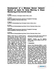
Figure 5: Average number of transmissions per node versus load (number of nodes with demand). total transmissions is equal to the number of transmissions and retransmissions made by a self-reporting node to try to send its data. In local systematic resource transfer, if a self-reporting node gets extra slots from its sub-network, the number of transmission is one, which is for sending a packet to inform the selected resource-supplier. If a self-reporting node gets extra slots from its parent’s sub-network, the total number of transmissions is two: one for sending an extra slot request to its parent and one for receiving extra slots from the parent. Furthermore, the total number of transmissions of a self-reporting node that tries to get extra slots from its neighborhood sub-networks is equal to the number of transmissions and retransmissions during contention in the FTS. Figure 5 shows local systematic resource transfer maintains a very low energy overhead compared to pure CSMA across diverse demand. In local systematic resource transfer, self-reporting nodes always try to get extra slots through FlexiMAC scheduled-communications before resorting to CSMA in the FTS. Whilst, in pure CSMA, as the demand increases, the contention increases and so results in high collision and retransmission. Figure 6 shows the percentage of unmet demand using either pure CSMA or local systematic resource transfer. As the demand increases, pure CSMA performance in supporting non-uniform sensing starts to deteriorate significantly, while local systematic resource transfer still meets around 90% of the demand. In pure CSMA, we calculated the percentage of self-reporting nodes in a network that are unable to send their data within the given period, which is equal to the FlexiMAC data gathering cycle period for that particular network. In local systematic resource transfer, we calculated the percentage of self-reporting nodes that are unable to get extra slots locally within a FlexiMAC data gathering cycle. Note that although a self-reporting node fails to get extra slots locally, it may get the slots centrally through central systematic resource transfer. 17
70 Local SRT Pure CSMA
60
Unmet demand (%)
50 40 30 20 10 0 10
20
30 40 50 Load (no. of self−reporting nodes)
60
70
Figure 6: Unmet demand versus load (number of nodes with demand). Load Unmet demand
50 0%
75 0.3%
100 0.5%
125 2.6%
150 3.7%
175 13.4%
Table 1: Unmet demand versus rapid data change load (number of nodes with demand). In the second experiment, we generated rapid data changes in 50 to 175 nodes in a network to measure the performance of central systematic resource transfer. In the experiment, a parent and its children in a sub-network reported similar sensor data. This sub-network state allows central systematic resource transfer to utilise the data aggregation technique when these nodes became self-reporting nodes. Thus, central systematic resource transfer can take even more demand. Table 1 shows the percentage of unmet demand using central systematic resource transfer versus rapid data change demand. As the demand increases, the supply of extra slots in the network decreases and so results in a reduced demand allocation. Simulation results show central systematic resource transfer satisfies more than 85% of the demand even in high demand cases.
8
Conclusions
We presented WinMS, an adaptive policy-based management system for wireless sensor networks. WinMS lightweight TDMA protocol, called FlexiMAC, provides energy-efficient management, data transport, and local repair. WinMS systematic resource transfer function allows non-uniform and reactive sensing in different parts of a network, and it provides automatic self-configuration and self-stabilization both locally and globally by allowing the network to adapt to current network conditions without human intervention. WinMS uses FlexiMAC to support resource transfer among nodes in the network and to ensure
18
slots are systematically transferred among nodes, maintaining low energy overhead and fast convergence. Using FlexiMAC, the network can be reconfigured and stabilized within a single data gathering cycle. The systematic resource transfer function can be executed locally or centrally. Autonomous sensor nodes perform the local systematic resource transfer function based on their local neighborhood state. Upon the occurrence of externally triggered events, a sensor node becomes a self-reporting node and initiates information exchange to try to get extra slots from nodes in its neighborhood. The central manager regularly analyses sensor data reported by all sensor nodes and performs the central systematic resource transfer function when it detects event triggers, providing the potential for better monitoring, control, and management of sensor networks. Our simulation results confirm that local systematic resource transfer function performs better than pure CSMA in terms of energy efficiency and capability to support non-uniform sensing. In the simulations, a self-reporting node only asks for one extra slot in a data gathering cycle. Clearly, pure CSMA will perform much worse if a self-reporting node asks for more than one extra slot. Furthermore, central systematic resource transfer performs well under varying demand, due to data aggregation and round-robin allocation strategy whenever the demand is higher than supply.
References [1] A. Mainwaring, J. Polastre, R. Szewczyk, D. Culler, and J. Anderson, “Wireless Sensor Networks for Habitat Monitoring,” in Proc. ACM WSNA Conf., Sep. 2002. [2] D. Estrin, L. Girod, G. Pottie, and M. Srivastava, “Instrumenting the World with Wireless Sensor Networks,” in Proc. IEEE ICASSP Conf., May 2001. [3] I. F. Akyildiz, W. Su, Y. Sankarasubramaniam, and E. Cayirci, “Wireless Sensor Networks: A Survey,” Computer Networks, vol. 38, no. 4, pp. 393– 422, 2002. [4] N. Xu, S. Rangwala, K. Chintalapudi, D. Ganesan, A. Broad, R. Govindan, and D. Estrin, “A Wireless Sensor Network for Structural Monitoring,” in Proc. ACM SenSys Conf., Nov. 2004. [5] W. Louis Lee, A. Datta, and R. Cardell-Oliver, “FlexiMAC: A Flexible TDMA-based MAC Protocol for Fault-tolerant and Energy-efficient Wireless Sensor Networks,” in To Appear in Proc. IEEE ICON Conf., Sep. 2006. [6] M. Turon, “MOTE-VIEW: A Sensor Network Monitoring and Management Tool,” in Proc. IEEE EmNetS-II Workshop, May 2005. [7] G. Tolle and D. Culler, “Design of an Application-Cooperative Management System for Wireless Sensor Networks,” in Proc. EWSN, Feb. 2005. 19
[8] B. Deb, S. Bhatnagar, and B. Nath, “Wireless Sensor Networks Management,” http://www.research.rutgers.edu/∼bdeb/ sensor networks.html, 2005. [9] B. Deb, S. Bhatnagar, and B. Nath, “A Topology Discovery Algorithm for Sensor Networks with Applications to Network Management,” Tech. Rep. DCS-TR-441, Rutgers University, May 2001. [10] B. Deb, S. Bhatnagar, and B. Nath, “STREAM: Sensor Topology Retrieval at Multiple Resolutions,” Kluwer Journal of Telecommunications Systems, vol. 26, no. 2, pp. 285–320, 2004. [11] A. Erdogan, E. Cayirci, and V. Coskun, “Sectoral Sweepers for Sensor Node Management and Location Estimation in Adhoc Sensor Networks,” in Proc. IEEE MILCOM Conf., Oct. 2003. [12] N. Ramanathan and M. Yarvis, “A Stream-oriented Power Management Protocol for Low Duty Cycle Sensor Network Applications,” in Proc. IEEE EmNetS-II Workshop, May 2005. [13] W. Liu, Y. Zhang, W. Lou, and Y. Fang, “Managing Wireless Sensor Network with Supply Chain Strategy,” in Proc. IEEE QSHINE Conf., Oct. 2004. [14] C. Hsin and M. Liu, “A Two-Phase Self-Monitoring Mechanism for Wireless Sensor Networks,” Journal of Computer Communications special issue on Sensor Networks, vol. 29, no. 4, pp. 462–476, 2006. [15] N. Ramanathan, E. Kohler, and D. Estrin, “Towards a Debugging System for Sensor Networks,” International Journal for Network Management, vol. 15, no. 4, pp. 223–234, 2005. [16] L.B. Ruiz, I.G. Siqueira, L.B. e Oliveira, H.C. Wong, J.M.S. Nogueira, and A.A.F. Loureiro, “Fault Management in Event-Driven Wireless Sensor Networks,” in Proc. ACM MSWiM Conf., Oct. 2004. [17] C-Y. Wan, S. B. Eisenman, A. T. Campbell, and J. Crowcrof, “Siphon: Overload Traffic Management using Multi-radio Virtual Sinks in Sensor Networks,” in Proc. ACM SenSys Conf., Nov. 2005. [18] J. Zhang, E.C. Kulasekere, K. Premaratne, and P.H. Bauer, “Resource Management of Task Oriented Distributed Sensor Networks,” in Proc. IEEE ICASSP Conf., May 2001. [19] M. Perillo and W.B. Heinzelman, “Providing Application QoS through Intelligent Sensor Management,” in Proc. IEEE SNPA Conf., May 2003. [20] A. Gonzalez, I. Marshall, L. Sacks, I. Henning, and T. Khan, “A SelfSynchronised Scheme for Automated Communication in Wireless Sensor Networks,” in Proc. IEEE ISSNIP Conf., Dec. 2004. 20
[21] G. Gupta and M. Younis, “Fault-Tolerant Clustering of Wireless Sensor Networks,” in Proc. IEEE WCNC Conf., Mar. 2003. [22] F. Koushanfar, M. Potkonjak, and A. Sangiovanni-Vincentell, “Fault Tolerance Techniques for Wireless Ad Hoc Sensor Networks,” in Proc. IEEE Sensors Conf., June 2002. [23] P. J. Marr´ on, A. Lachenmann, D. Minder, M. Gauger, O. Saukh, and K. Rothermel, “Management and Configuration Issues for Sensor Networks,” International Journal of Network Management, vol. 15, no. 4, pp. 235–253, 2005. [24] C. Intanagonwiwat, D. Estrin, R. Govindan, and J. Heidemann, “Impact of Network Density on Data Aggregation in Wireless Sensor Networks,” Tech. Rep. 01-750, University of Southern California, Nov. 2001. [25] J. Heidemann, F. Silva, C. Intanagonwiwat, R. Govindan, D. Estrin, and D. Ganesan, “Building Efficient Wireless Sensor Networks with Low-Level Naming,” in Proc. ACM SOSP Conf., Oct. 2001. [26] B. Krishnamachari, D. Estrin, and S. Wicker, “Modeling Data Centric Routing in Wireless Sensor Networks,” in Proc. IEEE INFOCOM Conf., June 2002. [27] W. Louis Lee, A. Datta, and R. Cardell-Oliver, “QMAC: A Quality of Service-Oriented Medium Access Control Protocol for Data Gathering in Wireless Sensor Networks,” Tech. Rep. UWA-CSSE-05-005, The University of Western Australia, Aug. 2005.
21