costs and the feasibility of management of hundreds of devices. .... RFID-based system able to locate and track personnel and machinery in mines ..... recording) cannot be easily distinguished, since the shapes of their PMFs ..... the energy content of the acquired signal, which can be evaluated in the time ...... Presto Parking.
1 Wireless Sensor Networks and Audio Signal Recognition for Homeland Security Abstract . . . . . . . . . . . . . . . . . . . . . . . . . . . . . . . . . . . . . . . . . . . . . . . . . . . . . . . . . . Keywords . . . . . . . . . . . . . . . . . . . . . . . . . . . . . . . . . . . . . . . . . . . . . . . . . . . . . . . . 1.1 Introduction . . . . . . . . . . . . . . . . . . . . . . . . . . . . . . . . . . . . . . . . . . . . . . . 1.2 WSNs for Menace Detection and Area Monitoring
1-1 1-1 1-2 1-2
Monitoring and Menace Identification • WSN Testbeds
1.3 Audio Signal Recognition Techniques for Surveillance of Critical Areas . . . . . . . . . . . . . . . . . . . . . . . . . . . . . . . . . . . . . . . . . . 1-5 Related Work • System Model • Training and Energy Detection
1.4 A Use Case Example of Wireless Sensor Networks for Homeland Security . . . . . . . . . . . . . . . . . . . . . . . . . . . . . . . . . . . . . . 1-9
Marco Martal` o E-Campus University, Novedrate (CO), Italy
Gianluigi Ferrari University of Parma, Italy
Claudio Malavenda Selex Sistemi Integrati S.p.A., Rome, Italy
The Architecture • Operational Highlights • Key Features
1.5 A Low-Complexity Hybrid Time-Frequency Approach to Audio Signal Pattern Detection . . . . . . . . . . . . . . . . . . . 1-12 Frequency-based Audio Pattern Recognition • The Hybrid Time/Frequency Algorithm • Performance Analysis
1.6 Concluding Remarks . . . . . . . . . . . . . . . . . . . . . . . . . . . . . . . . . . . . 1-24 Acknowledgment . . . . . . . . . . . . . . . . . . . . . . . . . . . . . . . . . . . . . . . . . . . . . . . 1-24
Abstract A plethora of solutions to homeland security problems have been proposed, during the last years, by academia, national governments, and industries. In this chapter, we focus on homeland security solutions based on efficient Wireless Sensor Network (WSN)-based audio signal pattern recognition. This is of interest for efficient surveillance of the perimeters of large areas, in order to detect the intrusion of humans or vehicles. We first propose a simple time domain approach to signal pattern detection and its commercial application through Unattended Ground Sensors (UGSs). Then, we extend this approach in the direction of a hybrid time-frequency approach, obtaining a very good performance yet with limited complexity.
Keywords Homeland security, surveillance, Wireless Sensor Networks (WSNs), data fusion, audio recognition. ISBN$0.00 c 2012 by CRC Press
1-1
1-2
1.1
Introduction
Recent years have witnessed a growing attention to the security of our daily lives, due to the recent experience of terrorist attacks. Therefore, a plethora of solutions to homeland security problems, either civilian or military [3], have been developed, from academia, national governments, and industries. One of the most critical aspects in homeland security is the requirement for non-invasiveness in security monitoring systems. To this end, Wireless Sensor Networks (WSNs) have been considered as a promising technology to increase homeland security from the very beginning, due their low costs and the feasibility of management of hundreds of devices. Typical WSN devices are equipped with a set of sensors useful for homeland security applications, e.g., audio, magnetic, movement, light, etc. Efficient processing and analysis of these data coming from different sensors are then required, with particular attention to the derivation of low computational complexity schemes. In the first part of this chapter, we overview the main WSN technologies, as well as the main design issues arisen in this field. As in various homeland security applications it is often of interest to process audio signals, e.g., for surveillance of the perimeters of critical areas, in the second part of this chapter we briefly review the main audio signal processing techniques for menace detection. In particular, we rely on time domain processing to identify the instant of appearance of an audio signal to be detected. Moreover, we present an implementation instance of WSN-based monitoring system for homeland security applications developed by an Italian company well established in the homeland and defense business sector. This monitoring system is based on networks of Unattended Ground Sensors (UGSs), micro devices with sensors and wireless connectivity that can detect movements, magnetic fields, audio signals, and combine this heterogeneous (yet correlated) information to generate proper events and alarms. In surveillance applications, the following problem is meaningful: detecting, with limited complexity, the presence and the pattern of an audio signal. We focus on the audio signal, since this is one of the physical quantities which can achieve high detection range, i.e., cover a large zone to be detected, although with a sufficiently small signal quality obtained from transducers. The two quantities are, in fact, related by an inverse proportional relationship. For instance, high level systems can even detect audio signals originated from sources at 15 Km [2]. The importance of audio processing in the military context is also reviewed together with some of the most important classification algorithms for this application in [33]. The data retrieved with the proposed audio recognition-based detection approach belongs to a larger set of sensed data, which are properly combined by means of data fusion techniques. However, in this chapter we limit ourselves to a detailed investigation of the audio sensor-based solution for menace recognition. We recall that our approach is not general and is “hard-linked” to resources available on a real sensor node (memory, computational power, synchronization capabilities, and power consumption). Several approaches (often computationally intense) have been proposed in the literature for audio signal pattern detection. Most of them rely on the analysis of the statistical properties of the audio signals. Unfortunately, in WSN-based surveillance scenarios, where nodes are typically batterypowered, the node energy consumption is a critical issue. Therefore, in the last part of this chapter we present a low-complexity approach, based on the combination of time- and frequency-based signal processing, to the audio recognition problem.
1.2 1.2.1
WSNs for Menace Detection and Area Monitoring Monitoring and Menace Identification
A first important task in designing WSN-based solutions for menace detection is to face the application domain of interest. According to the application to be implemented and the type of physical data to be measured, the particular menace can be categorized. From this broader point of view,
Wireless Sensor Networks and Audio Signal Recognition for Homeland Security
1-3
a menace can be interpreted as corresponding to a measure of the data quantity of interest out of its standard values or with an anomalous evolution during a given time period. For instance, if an area is being monitored to discover intruders, the menace will be classified as a fast physical measure variation in terms of terrain vibration or magnetic field anomaly near a sensor node. On the other hand, if a field is being monitored for agricultural purposes, the menace will correspond to an atypical increase of humidity or temperature in the area of interest. Another possible application example is traffic monitoring, where an anomaly may correspond to the increase, beyond a given threshold, of the number of cars passing by a traffic light. Once the application of interest has been identified, one can define the physical quantity to be measured, as well as its standard (non-critical) variability range and, consequently, the level of variability which constitutes a menace. Then, the menace has to be detected by means of proper data processing and/or fusion, in order to recognize the cause of the anomalies. Let us consider the examples introduced above. In the intrusion detection case, data coming from different sensors have to be gathered to recognize the type of intruder (e.g., a human, a small animal, or a vehicle). In the case of field monitoring, instead, the recognition activity could aim at detecting which kind of disease is spreading in order to select the appropriate pesticide to spray. Therefore, the operations needed to perform the menace recognition task can be summarized in the following two steps. • During the first step, bulks of data are acquired and eventually pre-processed. The main goal of this step is to acquire data only when an event of interest occurs. Data pre-processing aims at bringing all acquired data (coming from different sensors) into a common reference system. For instance, this operation may refer to a conversion of current/voltage values in a percentage scale. • The second step is refinement and involves the association, correlation, and combination of information obtained during the first step. The goal is to detect, characterize, and identify objects (including humans, animals, and vehicles). According to the scenario of interest, this step can be performed in a centralized or decentralized way. Algorithms should support data alignment and attribute estimation, as well as event positioning. In the following subsection, we review the most important available products that, according to the design principles given above, have been designed and commercialized by industries for relevant applications, such as intrusion detection, infrastructure monitoring, environmental monitoring, traffic control, aeronautics, industrial control, and system automation.
1.2.2
WSN Testbeds
A large number of WSN testbeds has been developed in academic environments, such as, for example, MoteLab [45] and WiseBed [19], but market-ready solutions are still not extensively available. In fact, most of the hardware production is still limited to a few companies that sell products effectively corresponding to development boards. Moreover, the offer of these companies is usually limited: a complete WSN solution, in fact, does not need only a hardware solution, but also firmware, protocols, sampling algorithm, and interface software. The different capabilities needed to develop each of these solution “ingredients” is maybe one of the major reasons behind the fact that a few market-ready and a rather small number of complete solutions exist. This is mainly due to the typically followed commercial practice, according to which the market responds to demands, rather than investing on potential solutions. The main applications fall in the agricultural field, border surveillance, and asset protection. Lately, however, urban monitoring has gained a significant attention, following the trend of formation of huge cities (only in China, for example, there are over 170 cities populated with over a million people each).
1-4 One player with a significant impact on the definition of the standards used in the development of sensor gateways is the Internet Protocol (IP) for Smart Object (IPSO) alliance [12]. The IPSO alliance focuses on the standardization of the Internet of Things (IoT) technologies and promotes the IP as the networking technology best suited for connecting smart objects and delivering information from and to those objects. The goal of the IPSO Alliance is not to define technologies, but to document the use of IP-based technologies defined by standardization organizations (such as the Internet Engineering Task Force, IETF) and support with various use cases. A first interesting WSN-based solution is Tinynode [14], which is mainly focused on vehicle (trucks and cars) detection. Tinynode consists of wireless battery-powered nodes together with Web-based applications. The system is claimed to yield at least 98% detection accuracy and at least 99% communication reliability. Nagios offers complete monitoring and alerting for IT infrastructures (servers, switches, applications, services, etc.) [7]. Its platform allows to monitor the entire IT infrastructure, preventing problems occurrence, becoming aware of the problems as they occur, providing security, etc. Netmagic also offers a platform for efficient infrastructure monitoring of IT systems [8]. Infrastructure monitoring enables to monitor availability and performance of IT systems so that managers can proactively take actions to maintain high uptimes: IT setup, provision of comprehensive information on the “health” of IT systems, thresholds, alerts, and reports. Advantic provides solutions for air quality, water, structural health, health monitoring, agriculture, environmental, energy efficiency, and mine monitoring [1]. In particular, the mine monitoring solution is an RFID-based system able to locate and track personnel and machinery in mines. Finally, Libelium provides solutions in several fields such as agriculture, environment, health, industrial processes, logistics, safety and emergency, and smart metering [6]. However, most of these application fields are only considered as proof of concept of the applicability of Libelium’s hardware (i.e., Waspmote) and protocol stack (Meshlium), but no practical monitoring solution has been presented. Other interesting active companies, especially in the field of smart cities and traffic control, are Urbiotica [15], Worldsensing [16], and Presto Parking [10]. In general, more and more products, from a growing number of manufacturers, are appearing in the global marketplace. Energy management is becoming the “killer application” and, thus, an efficient marketing motivation for home networking products. For instance, the KNX Association has published studies revealing how networked home and building control based on KNX allows up to 50% energy savings [34]. Interest has also been shown in energy management by other types of companies. For instance, Apple has filed patents for a device that could be used for energy management [29, 30]. In particular, the device links outlets into homes via power line networking, using HomePlug technologies [4]. With this approach, every outlet in the home turns into an Internet port, also allowing efficient power supply to connected devices. An interesting approach to the area monitoring problem is given by MasterZone, a product based on UGSs and developed by SELEX Sistemi Integrati [11]. The main focus of MasterZone is on border surveillance of large areas and its main target is the military market. MasterZone possesses the ability to detect the kind of intruder entering into a “hot” zone, distinguishing between human beings, animals, and vehicles. MasterZone can also be configured to monitor chemical and environmental parameters. In all cases, the collected information can be routed to a fixed or mobile sink. This solution will be described in detail in Section 1.4. To summarize, it seems that the provisioning of a commercial solution for area monitoring still requires a significant customization effort. In other words, most of the players in the WSN arena still wait for a specific customer demand to develop new solutions, rather than anticipating this demand with an offer. The difficulty in implementing effective large-scale solutions for area monitoring, also in “military” contexts, is witnessed by the cancellation of the virtual fence program after a one billion of USD-investment [39]. The virtual fence was a key element of the SBInet program [24], initiated in 2006, as part of the Secure Border Initiative (SBI) [25], to develop a new integrated system of personnel, infrastructure, and technology (such as WSN) to secure land borders of the
Wireless Sensor Networks and Audio Signal Recognition for Homeland Security
1-5
smart node (audio signal)
CRITICAL AREA 000000000000 111111111111 111111111111 000000000000 000000000000 111111111111 000000000000 111111111111 000000000000 111111111111 000000000000 111111111111 000000000000 111111111111 000000000000 111111111111 000000000000 111111111111 000000000000 111111111111 000000000000 111111111111 000000000000 111111111111 000000000000 111111111111 000000000000 111111111111 000000000000 111111111111 000000000000 111111111111 000000000000 111111111111 000000000000 111111111111 000000000000 111111111111
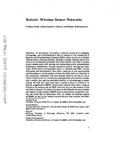
FIGURE 1.1
Illustrative representation of the audio signal recognition scenario of interest.
United States.
1.3
Audio Signal Recognition Techniques for Surveillance of Critical Areas
WSNs are typically equipped with a large variety of sensors and, therefore, it is possible to monitor an event of interest from different perspectives. As a practical example of area monitoring and menace detection, let us consider the detection of the presence of an undesired user in a critical zone. In this case, this detection can be performed by resorting to very different physical quantities obtained by different sensors, e.g., magnetic sensors, cameras, etc. Video signal processing is one of the key surveillance technologies and is, since long, well established. Video processing can be used, for instance, for face human recognition [20] or to detect and prevent possible critical situations [43, 31]. Real-time IP-based video processing for homeland security is proposed in [35], whereas an interesting summary of challenges is presented in [37]. The use of magnetic sensors for homeland security purposes is also attractive. In [18], the authors propose a new approach to assess the level of underwater security in civilian harbor installations, by means of the integration of a Geographical Information System (GIS) with acoustic and magnetic sensor models. A possible interesting approach is to identify the presence of a user by performing proper audio signal processing and determining if atypical sounds are present in the environment. In the remainder of this chapter, we will focus on audio signal processing for surveillance of critical areas. An illustrative representation of the scenario of interest is shown in Figure 1.1. Before presenting the system model and a low-complexity energy-based time domain processing approach, we overview related work.
1.3.1
Related Work
Sound recognition typically refers to the problem of determining which class a specific audio signal belongs to. Several approaches (often computationally intense) have been proposed in the literature and most of them rely on the analysis of the statistical properties of the audio signals. These approaches are typically based on the classification of some parameters of interest of the audio signals through Gaussian mixtures, hidden Markov models, or perceptron neural networks [27]. In [40], the authors propose an audio detection and classification scheme based on machine learning tech-
1-6 niques, which can outperform classical sound recognition schemes. In [46], the authors characterize the relevant spectral peaks of different audio patterns (for health care purposes) in order to perform the recognition task. In [22], an audio-based recognition system for gun shot detection is presented and its robustness against variable and adverse conditions is analyzed. Different time and frequency domain metrics for audio-based context recognition systems are analyzed in [28], comparing the system performance with the accuracy guaranteed by human listeners performing the same task. Particular emphasis is given to the computational complexity of the proposed methods, since the considered application is of particular interest in resource-constrained portable devices. Other interesting approaches to audio pattern recognition are presented in [17, 21]. Another interesting audio-related problem, widely studied in the literature, is the so-called Voice Activity Detection (VAD) problem. Unlike the previous problem of sound recognition, in this case one wants to detect the time intervals during which a (known) audio signal of interest (typically voice) appears, given that it will (sooner or later) appear for sure. A first possible strategy to detect the presence of an atypical audio signal, through a time domain-based analysis, consists in evaluating the energy of the audio signal samples, as in [44, 42]. Frequency domain-based VAD approaches have also been proposed through the application of the Discrete Fourier Transform (DFT) [38], as discussed in [26, 41, 32]. Although the performance of frequency domain processing algorithms can be better than that of time domain processing algorithms, the price to be paid is a higher amount of computational complexity. Therefore, the use of spectral analysis for VAD purposes is not recommended in WSNbased applications. Therefore, in the remainder of this section we focus on time domain processing for the identification of the presence of audio signal patterns of interest. Note, however, that spectral analysis is necessary when it is of interest to classify more precisely a detected atypical audio signal. This issue will be investigated in more detail in Section 1.5.
1.3.2
System Model
The front-end of the audio sensor (i.e., the microphone) is modeled as a linear filter with response H( f ), at the output of which the electrical signal x(t) can be written as follows: x(t) = r(t) ⊗ h(t) = sin (t) ⊗ h(t) + nin (t) ⊗ h(t) {z } | {z } | s(t)
(1.1)
n(t)
where r(t) = sin (t) + nin (t) is the input signal, sin (t) is the atypical audio signal of possible interest, nin (t) is the background audio noise, h(t) = F −1 [H( f )], and ⊗ denotes the convolution operator. The output signal x(t) is then sampled with frequency fs and the discrete-time samples are denoted as {xk }, with � sk + nk in the presence of an atypical signal xk ' (1.2) nk in the absence of any atypical signal where sk is the useful signal component and nk is the noise sample. More precisely, nk can be expressed as nk = nmic,k + nenv,k , where nmic,k is the noise generated by the microphone (on the order of 100 nV/Hz0.5 [5]) and nenv,k is the environmental audio noise. Typically, nmic,k � nenv,k . Our approach is based on per-frame processing, where a frame corresponds to a sequence of consecutive discrete-time samples. Denoting as K the number of samples per frame, the average per frame Signal-to-Noise Ratio (SNR) can be defined as follows: ∑Ki=1 |si |2 Evoice ∑K |si |2 = K K 2 = Ki=1 2 . SNR , Enoise ∑i=1 |ni | ∑i=1 |ni | K
(1.3)
Wireless Sensor Networks and Audio Signal Recognition for Homeland Security
1-7
Under the assumption that the noise is ergodic, its average energy Enoise at the denominator in (1.3) can be estimated during an initial training phase, when the background (noisy) audio signal is sensed but the system is still inactive for the purpose of pattern detection. Our approach can be extended to a more general scenario where the audio signal to be detected might be subject to filtering (i.e., to the presence of convolutional noise)· In other words, the recorded signal would be r(t) = g(t) ⊗ s(t) + n(t). (1.4)
Under the assumption of perfect estimation of g(t), considering an initial filter with impulse response g−1 (t), at its output one would have r0 (t) = s(t) + n0 (t)
(1.5)
where n0 (t) = n(t) ⊗ g−1 (t). The proposed detection strategy can be then applied, as its training phase takes automatically into account the statistical characteristics of n0 (t). In the case of unknown or time-varying channel impulse response g(t), one should first consider channel estimation, but this goes beyond the scope of this chapter.
1.3.3
Training and Energy Detection
The presence of an audio signal (of interest) can be identified by the “appearance” of an energy variation with respect to existing audio background noise. Therefore, one could first analyze the energies of consecutive audio signal frames in order to detect abrupt energy changes. This time domain-based approach is a direct extension of typical VAD approaches. The basic principle consists in comparing the average energy of a frame with a proper threshold Eth−initial , which depends 2 , respectively). on the mean and variance of the background noise energy (denoted as µlow and σlow Therefore, accurate estimation of the latter energy is fundamental and is the goal of the training phase. Denoting as Ntr−f the number of consecutive frames considered in the training phase and as N tr−s the number of samples per frame, the mean and the variance of the noise energy can be computed as follows:∗ tr−s N 1 tr−f 1 N (i) 2 (1.6) µlow , ∑ N tr−s ∑ xk Ntr−f i=1 k=1 �2 N N tr−s � 1 tr−f 1 (i) 2 2 σlow , (1.7) ∑ (N tr−s − 1) ∑ xk − µlow . Ntr−f i=1 k=1 low−s
Upon completion of the training phase, denoting as {xk }Nk=1 the N low−s samples in a generic collected frame, the following binary decision rule can be considered to determine the presence (Dlow = 1) or absence (Dlow = 0) of an “atypical” signal: low−s
∑Nk=1 |xk |2 N low−s
Dlow = 1
>
0 allowing to tune the sensitivity in detecting atypical signals. Our results show that ε = 1 allows to detect significant energy variations of the
∗ Note
that the correct unbiased estimator for small values of N tr−f is considered in the evaluation of the variance in (1.7). This is motivated by the fact that the number of collected frames in the training phase will be kept low, namely N tr−f = 20.
1-8 input audio signal, yet limiting the probability of missed detection. The impact of ε on the system performance will be investigated in Subsection 1.5.3. Note that if Dlow = 0 (i.e., no significant energy variation is detected), the average energy and the variance of the background noise can be adapted by taking into account the newly processed frame. In particular, the following adaptation rule can be used upon the reception of the `-th frame (` = 1, 2, . . .):
µlow (` + 1) =
µlow (` − 1) + µlow (`) 2
2 σlow (` + 1) =
2 (` − 1) + σ 2 (`) σlow low 2
(1.9)
2 (0) , σ 2 . This updating rule may be generalized considering a where µlow (0) , µlow and σlow low larger number of consecutive frames or varying the coefficients (now set to 1/2) of the linear combination in (1.9).∗ It can also be generalized in a decision-directed form with the smoothing parameter which can control the adaptation speed without any additional complexity and storage need. Note that the updates (1.9) are useful especially in the presence of non-stationary noise, with highly fluctuating variance. In this case, when no atypical signal is identified in the “triggered” fine processing phase (described in Subsection 1.5.1), the noise characteristics can be updated to better track the environmental changes.
By using the introduced energy-based processing, one can detect the presence of an atypical energy variation. However, our problem requires also to distinguish different audio signal patterns. As an illustrative example, we consider the following two discrete-time (ideal) audio signals: (i) the audio signal emitted by a M109 vehicle (a tank) moving at a constant speed of 30 km/h, with duration equal to 235 s and sampling frequency equal to 19.98 kHz, extracted from the NOISEX-92 database [9]; (ii) the audio signal of a choir singing the Handel’s “Hallelujah Chorus,” pre-loaded in Matlab with sampling frequency equal to 8.192 kHz [13]. Note that the Handel chorus, although unrealistic in surveillance applications, will be considered in this chapter only as representative of ideal human voice signals acquired at the highest sampling frequency with a microphone characterized by very good performance. The sequences obtained with different sampling rates are downsampled to a common rate, denoted as fslow , so that they can be additively combined. For each signal, we compute the normalized energy of each audio frame. The energy normalization is expedient to make the comparison meaningful—-in fact, if the average energy of one of the signals is much higher than that of the other, then distinguishing them is trivial. In Figure 1.2, the Probability Mass Functions (PMFs) of the frame energies are shown. The number of samples in the frame, denoted as N low−s , is set to 128. As one can see, the two audio signals (even in the presence of very accurate human voice recording) cannot be easily distinguished, since the shapes of their PMFs are very similar. This should be expected, since a VAD-inspired approach allows only to detect the time intervals where an atypical signal (e.g., the voice) is present, without giving any information about the “content” of the audio signal. Frequency domain-based approaches, typically based on the use of higher order statistics [26], have also been proposed for VAD. However, this significantly higher complexity is spent to detect more accurately the presence of atypical audio signals. In this case as well, if the energy distributions of the two audio signals are the same, their patterns cannot be distinguished. Therefore, increasing the computational complexity in this direction is, from the perspective of the problem at hand useless. In Section 1.4, we present a commercial product (MasterZone by Selex Sistemi Integrati) where the time-domain audio signal pattern detection algorithm described in Section 1.3 is implemented.
∗ Our
results show that updating the threshold by considering two consecutive frames allows to detect significant energy variations of the input audio signal with limited complexity.
Wireless Sensor Networks and Audio Signal Recognition for Homeland Security
1-9
0.18 Tank Handel Chorus
0.16 0.14 0.12 0.1 0.08 0.06 0.04 0.02 0 0.8
0.85
0.9
0.95
1 1.05 energy
1.1
1.15
1.2
FIGURE 1.2 Comparison between the tank signal and the Handel chorus. In this case, the PMFs of the per-frame energies are considered.
1.4
A Use Case Example of Wireless Sensor Networks for Homeland Security
In this section, we describe an industrial example of WSN used for homeland security. As already anticipated in Section 1.2, an interesting solution to a class of homeland security problems is given by the MasterZone system produced by SELEX Sistemi Integrati [11]. MasterZone, through the use of UGS technology, guarantees situational awareness and early warning. It supports force protection requirements and civil security needs, through the surveillance of target areas and the detection of hazards in different operational scenarios. The need of situational awareness calls for advanced solutions in support of surveillance and identification, in order to derive an accurate Common Operational Picture (COP) for decision makers. This objective is currently achieved by deploying personnel equipped with expensive and sophisticated platforms. These deployments are risky, particularly for the personnel, and expensive, in terms of maintenance cost. In order to mitigate the mission risks and increase the surveillance capability, SELEX Sistemi Integrati has developed MasterZone, a monitoring system based on UGS technology.
1.4.1
The Architecture
MasterZone is an advanced solution that meets the need of low-cost, low-power consumption and miniature sensors to ensure easy mass deployment, extended mission lifetime, and hand portability. A large quantity of sensor nodes can be deployed to cover a wide area and can routinely collect and report field information to command posts and personnel. MasterZone can be applied to several scenarios, by fulfilling crucial security, control, long-term monitoring and surveillance needs, with an advanced solution that reduces system complexity and costs. MasterZone applications include battlefield and force protection, critical infrastructure protection (airports and runways, industrial sites, utilities), access and border control, and illegal activities monitoring. A possible scenario of interest is depicted in Figure 1.3. In particular, in subfigure (a) a military application is envisioned, namely battlefield monitoring and army coordination. This kind of application is well known and analyzed by most of the literature in this realm. However, MasterZone can also be applied to a civil
1-10
FIGURE 1.3
Masterzone in illustrative (a) military and (b) civil context environment.
environment, as illustrated in subfigure (b), possibly integrating it with other surveillance systems, such as cameras with tracking capabilities. As an example, in subfigure (a) the application of interest is the control access of a civil manor. In this scenario, the ground sensor network is used together with a remote camera control, thus surrounding the civil manor with an “electronic fence.” When a menace is detected from the ground sensor network, an alarm can be raised toward a home central unit in the manor itself, or can be redirected toward a police station or another security agency. Being designed to operate in both open terrain and urban areas for critical targets’ detection and classification, MasterZone includes the following main functionalities. • Detection by sensors of anomalies, with alert activation, in terms of movements, sounds, magnetic fields variations, and terrain vibrations. • Data fusion activity and event generation performed by special nodes coordinating a given zone, denoted as “cluster head,” after receiving multiple warnings from the network. • Visualization of different alerts on the Monitoring Station, including geo-referentiation of the occurred threat, the involved sensing capabilities, and the most likely threat classification. Together with early warning, the data fusion activity provides a support to decision makers to discriminate people, vehicles, as well as any environmental perturbation. The standard MasterZone complete solution includes a network of short-range detection sensors and a central monitoring station for network monitoring and control. Default network sensing capabilities include seismic, infra-red radiations, magnetic field perturbation, temperature, pressure, and acoustics, but other types of sensors with additional sensing capabilities like gas, chemical, or nuclear waste detectors can be integrated. The modular sensor node consists of a CPU, a communication board implementing a proprietary communication protocol stack, and a sensor board to be configured in order to host one or more sensing capabilities, according to the context. Within the network, short range sensor nodes interact with each other, thus creating an ad-hoc wireless network. Nodes can automatically aggregate into clusters (short-range communication), and groups of clusters into a network (long-range communication). Within each cluster, a “cluster head” is elected and is responsible of the data fusion activity. Neighbour nodes are used as routers to convey data and information to the central monitoring station. The latter performs data acquisition from the network, as well as data processing and display of detected events, alarm generation, and threat evaluation by means of a 2D/3D Geographic Information System (GIS) interface.
1.4.2
Operational Highlights
The sensor nodes configuration for operational awareness is based on the following detectors:
Wireless Sensor Networks and Audio Signal Recognition for Homeland Security
(a) FIGURE 1.4
1-11
(b)
MasterZone: (a) tetrahedral and (b) box configuration.
• seismic (geophones), to identify ground vibrations caused by pedestrians or vehicles; • magnetic, to monitor movements of metal objects like vehicles; • acoustic, to detect the presence of targets (human, clusters of humans, military vehicles, etc.) by means of the time domain audio processing algorithm previously illustrated in Subsection 1.3.3; • passive infrared, to detect movements of objects in a narrow field of view; • Global Positioning System (GPS) receivers, for network geo-positioning. The main advantage of Masterzone, with respect to other solutions on the market, is a significant menace detection performance, owing to the fusion of multi-sensorial data collected by several small sensors scattered across a monitored area. Moreover, from audio signal processing perspective, coherently with the main core of this chapter, it is possible to integrate into Masterzone more advanced audio signal processing-based classification algorithms, such as that proposed in Section 1.5, which improves the low-complexity approach of Subsection 1.3.3 by using spectral audio signal “fingerprints.” This extension allows to distinguish different types of menace (vehicle from human, animals from humans, etc). However, it is not possible to have a finer identification capability, e.g., distinguishing a pair of adjacent humans from a single one. This is a subject of our current research activities. MasterZone is available in two configurations, shown in Figure 1.4, to fit different application requirements. The first configuration is denoted as tetrahedral: sensor nodes have four 10 cm (or even less) long legs. In this case, the sensor nodes can be easily deployed by dropping them from aircrafts, drones, or vehicles in hostile environments. The second configuration is denoted as box. In this case, the sensor nodes are cubes with 5 cm side and they have to be deployed manually. This configuration is thus suitable for civilian applications.
1.4.3
Key Features
MasterZone brings valuable benefits to a wide range of dual-use applications. The main advantages brought by the use of MasterZone can be summarized as follows. First, sensor nodes can be disseminated on the ground without any specific manual intervention and, therefore, with ease of
1-12 portability and deployability. This has been already observed with the tetrahedral configuration in Figure 1.4 (a). Moreover, the MasterZone architecture is highly flexible and scalable. In fact, MasterZone can be applied to a wide range of operational contexts demanding for enhanced protection and situational awareness. The open architecture and the use of sensor nodes leads to various scale solutions. Note also that MasterZone can operate in a standalone manner, as well as with other surveillance and identification systems, e.g., Closed-Circuit TeleVision (CCTV), video, Unmanned Aerial Vehicles (UAVs). Finally, the considered processing (e.g., data fusion at cluster-heads) allows to reliably avoid false alarms from sensors and the fault-tolerant configuration guarantees robustness and service continuity.
1.5
A Low-Complexity Hybrid Time-Frequency Approach to Audio Signal Pattern Detection
While the time-domain processing approach presented in Section 1.3 (from an algorithmic perspective) and Section 1.4 (from an industrial perspective) allows to detect the presence of an intruder, classifying the detected atypical audio signals requires further processing. In particular, our goal is to recognize if the detected abnormal signal belongs to a given class of interest. Referring to the homeland security problem, one possible envisioned application is to detect if a human (or a group of humans) enters a given area. Another possible application scenario consists in the detection of an unauthorized vehicle (e.g., a tank) entrance into a protected (forbidden) area. Our approach can be straightforwardly applied to other audio signals of interest (besides human and vehicles), provided that their frequency domain characteristics can be clearly identified and distinguished from those of other classes of audio signals. In this case, VAD-inspired approaches are no longer sufficient. In this section, we apply the ideas behind speech recognition techniques [32], typically used to recognize different spoken words, to classify different audio signal patterns. In particular, our key idea is that of characterizing an audio signal frame with a spectral signature and then, through frequency domain processing, detect if the received audio signal matches with the signature. In Subsection 1.5.1, the frequency domain processing is described. As the processing complexity might be very high, in Subsection 1.5.2 an innovative low-complexity hybrid time-frequency audio signal pattern detection algorithm is presented. Performance results are shown in Subsection 1.5.3.
1.5.1
Frequency-based Audio Pattern Recognition high−s
Upon the collection of the sequence of the samples of a single frame, denoted as {xk }Nk=1 high−s {X(n)}Nn=1 is computed:∗ N high−s
X(n) =
∑
2π − j high−s kn N
xk e
n = 1, . . . , N high−s .
, its DFT
(1.10)
k=1
The sequence {|X(n)|2 } is a particular instance of periodogram (in the absence of windowing between consecutive frames) associated with the sequence {xk } obtained by sampling the received high audio signal with a sampling rate denoted as fs . The sequence {|X(n)|2 } thus represents an accurate estimate of the signal power spectral density [38]. Since the computation of the periodogram
∗ Assuming
that N high−s is a power of 2, it is possible to efficiently compute the DFT through a Fast Fourier Transform (FFT). Note also that N high−s might, in general, be different from N low−s introduced in Subsection 1.3.2.
Wireless Sensor Networks and Audio Signal Recognition for Homeland Security
1-13
is computationally heavy (because of the presence of the squares of the modules of the DFT coefficients), we simply consider, as a representative “spectral shape” of the audio signal frame, the sequence of the modules of the DFT coefficients, i.e., {|X(n)|}. Obviously, the spectral shape depends on the particular SNR: in fact, in the presence of high SNR, i.e., high audio signal energy, the coefficients {|X(n)|} will be large, and vice versa for low SNR. Therefore, a “normalized” version of the spectral shape is needed to use the same spectral signature, regardless of the SNR. In particular, we propose the following normalized spectral shape: |Y (n)| , q
|X(n)|
n = 1, . . . , N high−s
high−s ∑N`=1 |X(`)|2
(1.11)
q N high−s |X(`)|2 is such that the energy of the spectral shape is where the normalization factor ∑`=1 high−s
N unitary, i.e., ∑n=1 |Y (n)|2 = 1, regardless of the SNR. The key principle of the proposed approach is to compare the normalized spectral shape of the frames of the received audio signal with a proper reference spectral signature (with unitary energy) of a frame of the reference audio pattern: if there is a “good agreement” between them, then the detected signal is declared of interest. In order to implement this strategy, the spectral signature and the “agreement” criterion have to be properly identified. Note that the proposed spectral signaturebased approach cannot be applied if the signature is not available. The identification of the spectral signature requires the availability of a sufficiently large number of frames of the audio signal pattern of interest. However, our results show that a “coarse” characterization of the spectral characteristics of the reference audio pattern (e.g., using a few frames) is sufficient to guarantee good performance. In the presence of non-stationary audio signals (e.g., voices), our results have shown that the best choice is to emphasize the high energy frequency components of the reference audio pattern. To this end, the best spectral signature of an audio pattern is typically given by the envelope of the sequence of normalized spectral shapes of the available frames of the reference audio pattern. The envelope over nframe consecutive frames can be defined as
I (nframe ) (n) =
max
i=1,...,nframe
|Yi (n)|
n = 1, . . . , N high−s
(1.12)
where |Yi | is the normalized spectral shape of the i-th frame. On the other hand, in the presence of stationary signals (e.g., tank signal), an “average” spectral signature (based on the average of the FFTs of the frames) may lead to better performance. In [36], we propose an efficient (recursive) approach to the extraction of an envelope spectral signature. The extension to the extraction of an “average” spectral signature is straightforward. As an illustrative example, we evaluate the (normalized) spectral signatures of the tank and the Handel chorus signals introduced in Subsection 1.3.2. The signatures are shown in Figure 1.5 in the case with N high−s = 128 samples per frame (using 128-point FFT). As one can see, unlike the PMFs of the corresponding energies (Figure 1.2), the spectral envelopes are clearly different. This suggests that the two audio signal patterns may be successfully distinguished using the proposed spectral signature-based approach. Once the spectral (envelope) signature has been extracted, upon reception of a given number of frames of an audio signal of potential interest, a partial spectral envelope can be derived and compared with the signature. In particular, one can evaluate the Mean Square Error (MSE) between the partial spectral envelope of the received signal and the spectral signature as a function of the number of processed frames. At the m-th step (m = 1, 2, . . .), the MSE is high−s
MSE(m) ,
N ∑n=1
(m)
|Irx (n) − I (n)|2 N high−s
(1.13)
1-14 0.7 Tank Handel Chorus
0.6 0.5 0.4 0.3 0.2 0.1 0 −2000 −1500 −1000 −500
0
500
1000
1500
2000
f [Hz] FIGURE 1.5 Comparison between the tank signal and the Handel chorus. In this case, the signals’ spectral signatures are shown. (m)
high−s
where {Irx (n)}Nn=1 is the partial spectral envelope of the received signal after processing m frames. In the presence of the reference audio pattern, i.e., the class of audio signals to be classified, (m) Irx (n) is an increasing function of m (∀n). Provided that the spectral signature I (n) is represen(m) tative of all possible instances of the class of audio signals of interest, i.e., I (n) ≥ Irx (n), ∀n, m, (m) one can thus conclude that MSE is a decreasing function of m: the signal is declared of interest when the MSE becomes lower than a given threshold. The following (per frame) situations are then possible: Correct Detection (CD), if the MSE becomes lower than the threshold given that there is the reference audio pattern; Missed Detection (MD), if the MSE does not become lower than the threshold given that there is the reference audio pattern; False Alarm (FA), if the MSE becomes lower than the threshold given that there is not the reference audio pattern. The value of the MSE threshold can be chosen according to the behavior of {MSE(m) }, as will be discussed in more detail in Subsection 1.5.3. We remark that the threshold value is a key parameter and has to be properly set in order to optimize the performance of the proposed detection algorithm. The definition of the normalized spectral shape in (1.11) entails the use of a normalization factor with a square root and square powers. The complexity of these operations may be too high (e.g., for in-sensor applications). Therefore, we propose another heuristic normalization factor given by the sum of the modules, leading to the following simplified (still normalized) spectral shape: |Y simp (n)| = high−s
|X(n)|
n = 1, . . . , N high−s
N high−s |X(m)| ∑m=1
(1.14)
so that the condition ∑Nn=1 |Y simp (n)| = 1 holds. In this case as well, the partial spectral envelope of the received signal after processing m frames is (m)−simp
Irx
simp
(n) , max |Yi i=1,...,m
(m)−simp
(n)|
n = 1, . . . , N high−s .
(1.15)
In [36], it is shown that {Irx (n)} can be recursively updated. The performance of the detection algorithm can then be evaluated in terms of the following Mean Linear Error (MLE): high−s (m)−simp (n) − I simp (n) ∑Nn=1 Irx (m) (1.16) MLE , N high−s
Wireless Sensor Networks and Audio Signal Recognition for Homeland Security
1-15
Nlow → high Dlow = 1 Flh 1
Dlow = 1
Dlow = 1 Flh Nlow → high
Flh 2
Dlow = 0
Dlow = 1
Dlow = 0 Flow
Fhigh
Nhigh−f �xed iterations (Nhigh−f frames olle ted)
Nhigh → low
Dhigh = 0 Fhl 4
Fhl Nhigh → low Dhigh = 0
Fhl 3 Dhigh = 0
Fhl 1
Fhl 2 Dhigh = 0
Dhigh = 0
Dhigh = 1 (Mat h with signature)
111111 000000 000000 111111 000000 111111 000000 111111 000000 111111 000000Alarm 111111
emission
FIGURE 1.6
FSM model for the proposed hybrid time-frequency audio signal pattern detection scheme.
where I simp (n) is the simplified spectral signature. Obviously, the MLE computation has a complexity much lower than that of the MSE. It can also be shown that, provided that the simplified spectral signature I simp (n) is representative of all possible instances of the class of audio signals (m)−simp of interest (i.e., I simp (n) ≥ Irx (n), ∀n, m), MLE(m) is a decreasing function of m. As in the (m) MSE case, when MLE becomes lower than a properly chosen threshold (different from the MSE threshold), one can declare that the detected signal is of interest. In the remainder of this chapter, the MLE threshold will be denoted as τhigh .
1.5.2
The Hybrid Time/Frequency Algorithm
We now present a low-complexity audio recognition algorithm whose focus is to detect, with limited complexity, the presence and the pattern of an audio signal. In this sense, our problem is related to both VAD and sound recognition (first, presence detection; then, pattern identification). In particular, we will show that our approach leads to the same performance of other approaches in the literature (e.g., that presented in [28]), but with a much lower computational complexity. The frequency domain-based approach proposed in Subsection 1.5.1 does not take into account the energy content of the acquired signal, which can be evaluated in the time domain with a much lower computational complexity. In fact, when the reference audio pattern is not present in the acquired audio signal, the energy of the acquired signal coincides with that of the background noise. Therefore, one may exploit this idea to significantly reduce the computational complexity as follows. First, the presence of a possible atypical signal is detected, in terms of energy variation, by using the simple time domain processing described in Subsection 1.3.3. Then, if an “atypical” signal is detected, its pattern is analyzed using the frequency domain processing technique described in Subsection 1.5.1. Taking into account possible correlations between consecutive frames, it is expedient to consider (as often done in VAD schemes [26]) a hangover Finite State Machine (FSM) model, shown in Figure 1.6, where the evolution between the state (Flow ) associated with coarse processing and the state (Fhigh ) associated with fine processing occurs through intermediate states. Every transition is a direct consequence of a single frame processing. In particular, the audio signal frames have fixed duration in each processing phase. Having fixed the frame duration, we denote as N low−s = low · f low and N high−s = T high · f high the numbers of samples per frame in the coarse and fine Tframe s s frame
1-16 high
processing phases, where fslow and fs are the sampling rates in the two phases, respectively. The sampling frequency fslow is low: namely, fslow < 2 fNyq , where fNyq is the Nyquist frequency of the audio signal at hand. This choice is not critical, since in the coarse processing phase our goal is simply to detect abrupt energy changes, but not an accurate signal reconstruction. On the high other hand, fs should be higher than 2 fNyq . However, in the experimental results presented in the following we will consider a microphone with a sampling frequency slightly lower value than 2 fNyq . Our results show that this does not hinder the performance—recall that the pattern, rather than the specific signal, needs to be detected—yet allowing to reduce the complexity. The evolution of the proposed processing algorithm over the FSM can be described as follows. Typically, the algorithm is in Flow . After low-complexity processing (in time domain) of an N low−s sample frame, a binary decision Dlow on the presence of an atypical signal is taken: if Dlow = 0 (no atypical signal), the algorithm remains in Flow ; if Dlow = 1, the algorithm evolves to the next intermediate state, denoted as Flh 1 , where low-complexity processing is considered. In general, lh low to Fhigh . one can consider Nlow → high intermediate states (Flh 1 , . . . , FNlow → high ) to evolve from F The use of the intermediate states is expedient to avoid useless and computationally intensive fine processing in the presence of impulsive noise, which may lead to short significant energy variations but, obviously, is not of interest. In the illustrative FSM model in Figure 1.6, Nlow → high is set to 3. If for Nlow → high + 1 consecutive frames the presence of an atypical signal is verified (i.e., Dlow = 1), then the algorithm moves to Fhigh . In this state, a fixed number Nhigh−f (to be properly selected, as discussed in Subsection 1.5.3) of frames, with N high−s samples each, is collected. After processing the Nhigh−f frames in the frequency domain, as described in Subsection 1.5.1, a binary decision Dhigh is taken: if Dhigh = 1 (i.e., MLE(Nhigh−f ) is below threshold), then the signal pattern is declared of interest, a proper alarm is emitted, and the algorithm moves back to Flow ; if Dhigh = 0, then the algorithm moves to an intermediate state Fhl 1 and processes one more frame. At this point, if Dhigh = 1, then the algorithm moves to Flow and an alarm is emitted; otherwise, it moves to the next intermediate state Fhl 2 . Eventually, if Dhigh = 0 for Nhigh→low + 1 consecutive frames (after exiting Fhigh ), then the algorithm comes back to Flow and no alarm is emitted: in other words, the atypical signal detected in the coarse processing phase is declared of no interest. The intermediate hl high to Flow can be interpreted as “back-up” states used to collect states {Fhl 1 , . . . , FNlow → high } from F a larger number of frames to be fine processed, in order to improve the reliability of the decision on the presence of a reference audio pattern. In the illustrative example in Figure 1.6, it holds that∗ Nhigh → low = 5. The derivation of a statistical model for the probability of FA would allow to analytically select the value of Nhigh → low . However, this extension goes beyond the scope of this chapter. We now present a comparative computational complexity analysis of the hybrid time-frequency approach proposed in this section with respect to the frequency domain-based approach presented in Subsection 1.5.1. To this end, suppose that the reference audio pattern is present only in a fraction α of the Nframe collected frames (typically, α � 1). If only frequency-based processing is performed, the total computational complexity can be quantified as follows: F Ctot = Nframe Cfreq
(1.17)
where Cfreq is the computational complexity of frequency domain-based processing of a single frame. When, instead, the hybrid time-frequency approach is considered, the overall computational complexity becomes T−F Ctot = αNframe Cfreq + (1 − α)Nframe Ctime (1.18)
∗ Typically,
in the VAD literature Nhigh → low > Nlow → high [26].
Wireless Sensor Networks and Audio Signal Recognition for Homeland Security
1-17
where Ctime is the computational complexity of time domain-based processing of a frame. Since time domain processing requires the computation of the per-frame average energy, its computational complexity (in terms of basic operations) is on the order of O(N low−s ), where N low−s is the number of per-frame samples. In fact, the computation of the per-frame average energy involves N low−s square operations, N low−s − 1 additions, and 1 division. Frequency based processing, instead, involves the computation of the FFT of the frame and a comparison with the pre-defined spectral signature: Cfreq = CFFT + Csig
(1.19)
high−s
where it is well known that CFFT ∼ O( N 2 log N high−s ) [23] and Csig ∼ O((N high−s )2 ) (because of the number of additions in (1.14)). Note that the signal power spectral density may be computed by means of the periodogram; in this case, however, no normalization is involved. Moreover, the complexity associated with this operation is negligible with respect to that of the FFT computation. At this point, one obtains F Ctot T−F Ctot
= Nframe (N high−s )2 = αNframe (N high−s )2 + (1 − α)Nframe N low−s ' αNframe (N high−s )2
(1.20) (1.21) (1.22)
where we have used the fact that, typically, N low−s � N high−s . After a few simple manipulations, the complexity reduction brought by the use of the hybrid time-frequency pattern detection algorithm is on the order of F 1 Ctot ' � 1. T−F α Ctot
(1.23)
This is intuitively expected, since the hybrid approach concentrates the complexity only in the presence of an atypical signal. If the atypical signal is of interest and appears for a fraction α of the time, then the complexity reduction is on the order of 1/α. We remark that the complexity of the frequency domain processing approach of Subsection 1.5.1 is comparable to other existing frequency domain-based algorithms (e.g., [28]). Therefore, the complexity reduction brought by the proposed hybrid approach holds also with respect to them.
1.5.3
Performance Analysis
“Ideal” Signals
The following set-up is considered. The potential audio signals of interest are the Handel chorus and the tank sound, introduced at the end of Subsection 1.3.3. A “slice” of the reference audio pattern is 8 s long and is randomly additively combined with a background noisy audio signal of duration equal to 235 s and sampling frequency equal to 19.98 kHz, extracted from the NOISEX92 database [9]. On top of the background noisy signal, a slice of another audio signal (with a spectral signature different from that of the reference audio pattern) is inserted. The two slices do not overlap: otherwise, our system would not be able to detect any of them. The training phase is carried out considering Ntr−f = 20 frames of the background noisy signal. The sampling frequencies high for the coarse and fine processing phases are fslow = 1024 Hz and fs = 4096 Hz, respectively. As anticipated in Subsection 1.3.3, the audio sequences (tank, Handel chorus, and background noise) obtained with different sampling rates are downsampled to fslow = 1024 Hz in the coarse processing
1-18 7
7
Tank (nuisance signal)
6 5
5
MSE 4
MLE 4
3
3
2
2
1 0 0
Handel Chorus (signal of interest) 5
10
N high−f
(a)
Tank (nuisance signal)
6
Handel Chorus (signal of interest)
1
15
20
0 0
5
10
N high−f
15
20
(b)
FIGURE 1.7 MSE and MLE, as functions of the number of frames, in a scenario with the Handel chorus as reference audio pattern. high
phase∗ and to fs = 4096 Hz in the fine processing phase. The numbers of samples per frame analyzed in the coarse and in the fine processing phases are N low−s = 16 and N high−s = 128, so that low ' 16 ms and T high ' 31 ms, respectively. the frame durations in the two phases are equal to Tframe frame The numbers of intermediate states in the FSM have been heuristically set to Nlow→high = 3 and Nhigh→low = 5. The filter that will first be considered, in our simulations, to process ideal audio signals is derived from a Low-Pass Filter (LPF) of the commercial microphone which will be used to collect realistic audio signals [5], as described in more detail in Subsection 1.5.3. In order to approximate this LPF, we use a Butterworth Infinite Impulse Response (IIR) filter with a 3 dB bandwidth approximately equal to 2.2 kHz. We assume that the Handel chorus is the reference audio pattern, whereas the tank audio signal is not.∗ The background noise is assumed Gaussian and white. As a first analysis step, we investigate the behaviors of the MSE and MLE (between the partial envelope of the received signal and the spectral signature) as functions of number of collected frames. To this purpose, the SNR is set to 20 dB. In order to evaluate the system performance, we perform 20 independent simulation runs (with random generation of disjoint initial time instants of the Handel chorus and tank audio signals). In Figure 1.7 (a), the MSE is shown, as a function of the number of processed frames. It is possible to observe that the set of curves associated with the reference audio pattern is lower than that associated with the pattern of no interest. This behavior is pronounced also for a small number of frames: for instance, after 3 frames, the signals are easily separable. In other words, the proposed spectral signature-based detection approach is effective also when a few frames are collected and analyzed. In Figure 1.7 (b), the MLE is considered. Although a general performance degradation (in terms of separability) can be observed (due to the simpler normalization), the reference pattern (Handel chorus) can still be distinguished from the other one (tank). From the results in Figure 1.7, one can determine the number of frames Nhigh−f which need to be processed, in the state Fhigh of the FSM, in order to reliably recognize the identified audio pattern. Simultaneously, the corresponding value
∗ We consider a very small value of f low in order to reduce the computational complexity, thus saving as much battery s energy as possible in wireless sensor network-based applications. ∗ Note that similar results hold in a scenario where the tank signal is of interest and Handel chorus is not. They are not reported here for lack of space.
1-19
Wireless Sensor Networks and Audio Signal Recognition for Homeland Security 5
1 0.9
Nhigh-f = 1 - Handel chorus Nhigh-f = 5 - Handel chorus
4
0.8 0.7
Nhigh-f = 1 - Tank
PCD
0.6
Nhigh-f = 1, Handel chorus Nhigh-f = 5, Handel chorus
P 0.5
Nhigh-f = 1, Tank
0.4 0.3
[s]
Nhigh-f = 5, Tank
PMD
Dest
Nhigh-f = 5 - Tank
3 2 1
0.2 0.1 0 0
4
8 SNR [dB]
12
16
0 0
4
(a)
8 SNR [dB]
12
16
(b)
FIGURE 1.8 Probabilities of MD and CD (case (a)) and delay in the presence of CD (case (b)), as functions of the SNR, in a scenario with Handel chorus or tank as reference audio pattern and MLE-based frequency domain processing. Two possible values for Nhigh−f are considered: 1 and 5.
of the threshold τhigh can be determined as a function of the selected value of Nhigh−f . For instance, if Nhigh−f = 5, then τhigh ' 2.5. Reducing Nhigh−f , τhigh should increase. However, our results show that a higher value of τhigh makes the probability of FA increase dramatically. Therefore, for Nhigh−f < 5, the best performance is obtained with a “conservative” value of τhigh equal to 2.5. In Figure 1.8 (a), the probabilities of MD and CD are shown, as functions of the SNR, in a scenario with Handel chorus or tank as reference audio pattern and MLE-based frequency domain processing. Two possible values for Nhigh−f are considered: 1 and 5. For every value of SNR, 1000 independent simulation runs are performed, in order to eliminate possible statistical fluctuations. The background audio noise is Gaussian and white. One can note that approximately the same performance can be observed for both signals of interest. In particular, for sufficiently high values of the SNR (around 8 dB) the probability of MD goes to zero, whereas the probability of CD goes to 1. One may argue that this value is too high; however, it is possible to observe that for SNR≥ 4 dB the probability of MD is already below 10%. Moreover, as it will be shown in the next subsection, the penalty with respect to “classical” frequency-based algorithms is limited. Moreover, for low values of the SNR, increasing the number of frames in the fine processing phase allows to improve the performance. For Nhigh−f = 5, however, one can observe some fluctuations in the probability of CD. In this case, some false alarms, even if rare (with probability on the order of 10−2 ), appear at intermediate SNR values and disappear for large values of the SNR. This is due to the fact that for large values of Nhigh−f , the considered value of τhigh may not be optimal for these intermediate SNRs. In general terms, one can consider that the detection algorithm is properly working when the probability of CD becomes significantly higher than the probability of MD. For instance, in the scenario considered in Figure 1.8 the proposed detection algorithm becomes effective for SNR ≥ 7 dB. In Figure 1.8 (b), the delay (dimension: [s]) is considered. The delay is evaluated only when there is CD, since, otherwise, it would not be meaningful. In fact, when the pattern is not identified, the state of the system continuously iterates, in the FSM, between the coarse and fine processing states.∗ For small values of the SNR, the delay is around 4 s and it would not be possible to detect signals with duration shorter than this maximum delay—recall that the entire duration of the signal
∗ One
may consider a maximum number of iterations after which the system is reset.
1-20 “slice” of interest is 8 s. This is due to the large number of frames which are processed before the presence of an atypical signal is declared in the coarse processing phase. For large values of the SNR, instead, in 0.5 s the reference audio pattern if correctly identified, thus making the proposed algorithm almost real-time. One can observe that the delay depends only slightly on the number of processed frames. The limiting lower value of the delay for large values of the SNR is due to the fact that, even in the presence of correct identification, Nlow→high + 1 frames (with low sampling frequency) and Nhigh−f frames (with high sampling frequency) need to be processed, thus leading to the following minimum achievable delay: high
low Dmin = (Nlow→high + 1)Tframe + Nhigh−f Tframe .
(1.24)
Expression (1.24) holds for sufficiently large values of Nhigh−f (e.g., Nhigh−f = 5). For Nhigh−f = 1, instead, the delay is slightly large, since more backup frames need to be processed before a spectral match is declared (i.e., the MLE lowers below threshold). In other words, a single frame is not sufficient in Fhigh and it may happen that the system state starts moving back towards Flow before declaring a match. Experimentally Acquired Signals
We now analyze the performance of the proposed audio pattern detection algorithm in the presence of signals acquired through the realistic microphone mentioned in Subsection 1.3.2. We remark that this microphone is characterized by a flat frequency response and its sampling frequency is high in the fine processing equal to 3450 Hz [5], which has been used as the sampling frequency fs phase for all audio sequences. Moreover, the acquired audio sequences are further downsampled to fslow = 1024 Hz in the coarse processing phase. The other simulation parameters are set as described at the beginning of Subsection 1.5.3. The performance is analyzed either (i) considering direct use of the signal at the output of the microphone or (ii) filtering the signal at the output of the filter through the front-end LPF, with cut-off frequency equal to 2.2 kHz, introduced in Subsection 1.3.2. The use of this LPF allows to derive preliminary insights on the impact of front-end digital filtering on the performance of the proposed detection algorithm. Further research is needed to derive the “optimal” front-end filtering technique. The acquired speech signals used to derive the spectral signature correspond to the voices of 5 males (with ages between 23 and 35, at the University of Parma) reading some texts, both in Italian and in English. Since the frequency response of the real microphone between 0 Hz and 100 Hz is not declared by the manufacturer [5], in the fine processing phase the FFT of each frame is set to zero in the [0,100] Hz band. As non-speech signal, we have acquired the sound emitted by the engine of a non-moving car (FIAT Punto, 1900 cc, turbo-diesel) running at 3000 rpm. The duration of all acquired signals is around 30 s. Note that these experimentally acquired signals are recordered in very noisy environments, e.g., open spaces (the university campus) or university laboratories, where these signals are mixed with different environmental noises. Therefore, these signals may be representative of signals of interest with reduced energy in surveillance applications. The spectral signature of the car engine can be uniquely extracted. On the other hand, when a speech signal is of interest, three possible approaches can be followed to extract a spectral signature: (1) compute the spectral envelope (as described in Subsection 1.5.1) associated with the available frames of the voice signal of the specific person to be detected; (2) compute the spectral envelope associated with the available frames of the voice signal of a person different from the one to be detected; (3) compute the arithmetic average of the spectral envelopes associated with all persons (speaking in Italian or English). Although similar results hold for cases (1) and (2), in the following we focus on case (3). This choice is motivated by the fact that the system should be robust against possible variations of the signals to be detected, i.e., we ideally want to be able to detect all audio signals belonging to
1-21
Wireless Sensor Networks and Audio Signal Recognition for Homeland Security 0.22
0.22 Car engine sound Human voice
0.2 0.18
0.18
0.16
0.16
0.14
0.14
0.12
0.12
0.1
0.1
0.08
0.08
0.06
0.06
0.04
0.04
0.02
0.02
0 −1500
−1000
−500
0
500
1000
1500
Car engine sound Human voice
0.2
0 −1500
−1000
−500
0
f [Hz]
f [Hz]
(a)
(b)
500
1000
1500
FIGURE 1.9 Spectral envelopes for speech and car engine signals. In case (a), the envelopes are compared in the presence of the LPF, whereas in case (b) the LPF is not considered.
the same class (e.g., human voice) with a single spectral signature. The 8 s speech signal slices, randomly additively combined with a background white noise signal in the simulator, correspond to other people reading different scripts. First, we analyze the impact of the presence of the front-end LPF. In Figure 1.9, the spectral signatures for speech and car engine signals are compared (a) in the presence and (b) in the absence of the LPF, respectively. One can observe that the presence of the LPF significantly changes the signature shape for both voice and car signals. In particular, the secondary peaks of the voice spectral signature, well evidenced in the absence of the LPF, become less evident if the LPF is considered. At this point, one could think that the use of the LPF is not beneficial, since the spectral signatures of the two audio signals seem to become less different. This, however, is not the case, as will be discussed later. In Figure 1.10, the MLE is shown, as a function of the number of processed frames, in a scenario with SNR = 20 dB for (a) speech or (b) car engine sound as signals of interest. The presence of the front-end LPF is considered and 20 independent simulation runs are performed. In case (a), the two groups of curves are well separated: if Nhigh−f is set to 15, then the MLE threshold τhigh (to be used in Fhigh ) can be set to 2.6. In case (b), instead, the audio pattern identification is more complicated, since the two groups of curves are not well separated. The absence of the front-end LPF leads to a performance degradation, i.e., the curves associated with different classes of audio signals cannot be easily distinguished and the MLE decision threshold increases—the results are not reported here for the sake of conciseness. For instance, in the case of speech signals of interest, the optimized value of τhigh becomes approximately equal to 4. This seems to be in contradiction with the results in Figure 1.9, from which one may think that the absence of evident secondary peaks in the presence of the LPF would not help in distinguishing between different patterns. However, the faster convergence in the presence of the LPF allows to conclude that concentrating the energy in the primary peaks might be more beneficial for the proposed detection algorithm. As previously anticipated, the design of the “optimal” LPF is an open problem. In Figure 1.11 (a), the probabilities of MD and CD and (b) the delay, in the presence of CD, are shown as functions of the SNR. The reference audio pattern is the speech. Both the presence and the absence of the front-end LPF are considered. On the basis of the analysis carried out in Figure 1.10, during the fine processing phase Nhigh−f = 15 frames are collected and the MLE threshold τhigh is set, in the presence and absence of the LPF, to 2.4 and 3.9, respectively. The values of the threshold have been reduced, with respect to those predicted by the results in Figure 1.10 (i.e., 2.6 and 4,
1-22
3.8
2
Car engine sound (nuisance signal)
3.6 3.4
MLE
1.8
3.2
1.6
3
MLE 1.4
Human voice (nuisance signal)
2.8 1.2
2.6 2.4
1
2.2 2
Human voice (signal of interest)
1.8 0
5
Car engine sound (signal of interest)
0.8
10
N high−f
15
0.6 0
20
5
10
N high−f
(a)
15
20
(b)
FIGURE 1.10 MLE, as a function of the number of processed frames, in a scenario with SNR = 20 dB for (a) speech or (b) car engine as reference audio pattern, respectively. The presence of the front-end LPF is considered.
1
4
W/o LPF
0.9
PMD PCD
0.8 0.7
Simulation (Dest) Weighed (D)
3
0.6
W LPF
P 0.5
W/o LPF
D [s] 2
0.4 0.3
1
0.2 0.1 0 0
W LPF
4
8
12 SNR [dB]
(a)
16
20
0 0
4
8
12 SNR [dB]
16
20
(b)
FIGURE 1.11 Performance with speech reference audio pattern: (a) probabilities of MD and CD and (b) delay, in the presence of CD, as functions of the SNR. Both the presence and the absence of the front-end LPF are considered.
1-23
Wireless Sensor Networks and Audio Signal Recognition for Homeland Security 1
5
0.9 0.8 0.7 0.6 P 0.5
4 PMD - frequency-based [32] PCD - frequency based [32]
3
PMD - hybrid time/frequency
D [s]
PCD - hybrid time/frequency
0.4
2
0.3 0.2
Simulation (Dest) - frequency-based [32]
1
Weighed (D) - frequency-based [32]
0.1
Simulation (Dest) - hybrid time/frequency Weighed (D) - hybrid time/frequency
0 0
4
8
12 SNR [dB]
(a)
16
20
0 0
4
8
12 SNR [dB]
16
20
(b)
FIGURE 1.12 Performance with speech reference audio pattern and absence of LPF: (a) probabilities of MD and CD and (b) delay, in the presence of CD, as functions of the SNR. The frequency-based algorithm in [28] is compared to the proposed hybrid time/frequency algorithm.
respectively), to lower the probability of FA. In general, τhigh should be tuned for the particular environment where the audio sensors are placed. Comparing the results in Figure 1.11 (a) with those in Figure 1.8 (a), one can observe that the trends are similar. In the current scenario, the absence of the LPF is detrimental, since the probability of CD reaches 1 for larger values of the SNR. Comparing the results in Figure 1.11 (b) with those in Figure 1.8 (b), the following observations can be carried out. Unlike in Figure 1.8 (b), in Figure 1.11 (b), for small values of the SNR, the simulated delay decreases. This is due to the fact that the number of correct detections also reduces (according to the behavior of the probability of CD in Figure 1.11 (a)). In this case, a weighed average delay between the estimated delay (in the presence of CD) and a pre-determined maximum delay Dmax (in the absence of CD) , defined as D , Dmax (1 − PCD ) + Dest PCD , is more meaningful. In Figure 1.11 (b), a maximum delay Dmax = 4 s is considered. As expected, the D curves compare favorably with the delay curves in Figure 1.8 (b). In Figure 1.12, (a) the probabilities of MD and CD and (b) the delay (in the presence of CD) are shown, as functions of the SNR, in the absence of LPF. The proposed hybrid time/frequency algorithm is compared to the frequency-based detection algorithm in [28], with spectrum quantization in 8 sub-bands. It is possible to observe that there is a performance degradation with respect to the scenario presented in Figure 1.11, due to the fact that the spectrum is quantized with a smaller number of points. One can note that the performance loss, in terms of probabilities of FA, MD, and CD, incurred by the hybrid approach is very limited (on the order of a fraction of dB). However, the delay with the proposed hybrid approach is lower than that with the frequency-based approach. This is due to the fact that in the latter case the system spends more time processing frames without energy atypicalities and this might delay the recognition of the pattern of interest. We now focus on the detection of the car engine audio signal. From the analysis of the MLE behavior in Figure 1.10 (b), the optimized value of τhigh is around 1.1. However, this value leads to a probability of FA too high and smaller values have to be considered. If τhigh = 0.9 is considered, PMD goes to zero for increasing SNR: however, PFA is too high and PCD too low. Reducing τhigh has a beneficial impact on PFA , but PMD does not go to zero any longer. This dismal performance is probably due to the fact that the FFTs of the frames are set to zero in the [0,100] Hz band, where the car engine signal energy concentrates. We finally investigate the impact of the sensitivity parameter ε in the VAD detection. In Figure 1.13, the probability of CD is shown, as a function of ε, in a scenario with speech as reference audio pattern and absence of front-end LPF. Two values for the SNR are considered: 8 and 14 dB.
1-24 1 0.9 0.8 0.7 0.6 PCD 0.5
SNR = 14 dB
0.4
SNR = 8 dB
0.3 0.2 0.1 0 0
0.5
1 ε
1.5
2
FIGURE 1.13 Probability of CD, as a function of ε , in a scenario with speech as reference audio pattern and absence of front-end LPF. Two values for the SNR are considered: 8 and 14 dB.
As one can see, the optimum value of ε depends on the considered SNR, but it is always in the range (0,1). However, the common choice ε = 1 allows to obtain a performance close to the best value for all possible values of the SNR.
1.6
Concluding Remarks
In this chapter, we have discussed WSN-based solutions for homeland security, e.g., applications like surveillance of critical areas. While we have first analyzed the main commercial WSN-based solutions for monitoring, we have then discussed one particular sensor processing for homeland security, i.e., audio processing for the detection of the presence of undesired users, showing a use-case example, i.e., MasterZone, where audio time-domain signal recognition is implemented. Finally, we have presented an innovative hybrid time-frequency audio signal pattern recognition. Our results show that the reliability of the proposed hybrid algorithm is very high, with limited computational complexity, thus making this solution suitable for WSN-based solutions for homeland security, e.g., MasterZone.
Acknowledgment This work was funded by Elsag-Datamat S.p.A. (ED), Rome, Italy, later become Selex Sistemi Integrati S.p.A. We would like to thank the “SISTEMI SPECIALI” working group directed by Claudio Marchesini, its account manager Paolo Proietti, and all its management staff Luca Di Donato e Sandro Matticci for the useful discussion on audio signal processing.
Bibliography 1. Advantic Systemas Y Servicios. URL: http://www.advanticsys.com/. 2. HALO: Hostile Artillery Locating System. URL: www.selexgalileo.com/EN/Common/files/ SELEX Galileo/Products/HALO.pdf. 3. Homeland Security. URL: http://en.wikipedia.org/wiki/Homeland security. 4. HomePlug Power Alliance. URL: https://www.homeplug.org/. 5. Infineon SM310. URL: http://www.infineon.com/. 6. Libelium. URL: http://www.libelium.com/. 7. Nagios. URL: http://www.nagios.org/. 8. Netmagic. URL: http://www.netmagicsolutions.com/. 9. NOISEX-92, Noise Database. URL: http://www.speech.cs.cmu.edu/ comp.speech/Section1/Data/noisex.html/. 10. Presto Parking. URL: http://www.prestoparking.com/. 11. Selex Sistemi Integrati. URL: https://www.selex-si.com/. 12. The IPSO Alliance. URL: http://www.ipso-alliance.org/. 13. The MathWorks - MATLAB. URL: http://www.mathworks.com/. 14. Tinynode: Real Life Wireless Sensor Networks. URL: http://www.tinynode.com/. 15. Urbiotica: The City Operating System. URL: http://www.urbiotica.com/. 16. Worldsensing: Making Smart Cities Happen. URL: http://www.worldsensing.com/. 17. Abu-El-Quran, A. R., R. A. Goubran, and A. D. C. Chan. 2006. Security monitoring using microphone arrays and audio classification. IEEE Trans. on Instrumentation and Measurement 55(4):1025–1032. 18. Caiti, A., A. Munafo, and G. Vettori. 2012. A geographical information system (GIS)based simulation tool to assess civilian harbor protection levels. IEEE J. Oceanic Engineering 37(1):85–102. 19. Chatzigiannakis, I., C. Koninis, G. Mylonas, S. Fischer, and D. Pfisterer. 2009. WISEBED: an open large-scale wireless sensor network testbed. In Proc. int. conf. on sensor networks applications, experimentation and logistics. Athens, Greece. 20. Chellappa, R., P. Sinha, and P. J. Phillips. 2010. Face recognition by computers and humans. IEEE Trans. Comput. 43(2):46–55. 21. Chu, S., S. Narayanan, and C.-C. J. Kuo. 2009. Environmental sound recognition with time-frequency audio features. IEEE Trans. Acoust., Speech, Language Processing 17(6): 1142–1158.
1-2
BIBLIOGRAPHY
22. Clavel, C., T. Ehrette, and G. Richard. 2005. Events detection for an audio-based surveillance system. In Ieee int. conf. on multimedia and expo (icme), 1306–1309. 23. Cooley, J., and J. Tukey. 2008. An algorithm for the machine calculation of complex Fourier series. Math. Comput. 19(90):297–301. 24. Customs, U.S., and Border Protection. . SBInet: URL: http://www.dhs.gov/xlibrary/assets/ sbinetfactsheet.pdf.
Securing U.S. Borders.
25. ———. . Secure Border Initiative. URL: www.cbp.gov/xp/cgov/border security/sbi/. 26. Davis, A., S. Nordholm, and R. Togneri. 2006. Statistical voice activity detection using low-variance spectrum estimation and an adaptive threshold. IEEE Trans. Acoust., Speech, Language Processing 14(2):412–424. 27. Dufaux, A. 2001. Detection and recognition of impulsive sound signals. Ph.D. thesis, Institute of Microtechnology—University of Neuchatel, Switzerland. 28. Eronen, A. J., V. T. Peltonen, J. T. Tuomi, A. P. Klapuri, S. Fagerlund, T. Sorsa, G. Lorho, and J. Huopaniemi. 2006. Audio-based context recognition. IEEE Trans. Acoust., Speech, Language Processing 14(1):321–329. 29. Fadell, A. 2010. Intelligent power-enabled communications port. US Patent 0007473. 30. ———. 2010. Intelligent power monitoring. US Patent 0010857. 31. Hampapur, A. 2008. Smart video surveillance for proactive security. IEEE Trans. Signal Processing 25(4):134–136. 32. Junqua, J.-C., and J.-P. Haton. 1995. Robustness in Automatic Speech Recognition: Fundamentals and Applications. Kluwer Academic Publishers. 33. Kaushik, B., D. Nance, and K. K. Ahuja. 2005. A review of the role of acoustic sensors in the modern battlefield. In Proc. AIAA/CEAS aeroacoustics conference, 1–4. Monterey, CA, USA. 34. KNX Association. Reduced energy consumption by using home and building control systems. URL: http://www.knx.org/knx/knx-applications/knx-is-green/. 35. Liu, H., C. Tang, S. Wu, and H. Wang. 2011. Real-time video surveillance for large scenes. In Int. conf. wireless comm. and signal (wcsp), 1–4. Nanjing, China. 36. Martal`o, M., G. Ferrari, and C. Malavenda. 2010. Low-complexity in-sensor audio detection with experimental validation. In IEEE int. symposium on industrial electronics (isie), 1674–1679. Bari, Italy. 37. Maybury, M. 2009. Audio and video processing to enhance homeland security. In IEEE Conf. Technologies for Homeland Security (HST), 516–523. Boston, MA, USA. 38. Oppenheim, A. V., and R. W. Schafer. 1989. Discrete-Time Signal Processing. Englewood Cliffs, NJ, USA: Prentice-Hall. 39. Preston, J. 2011. Homeland security cancels “virtual fence” after $1 billion is spent. The New York Times A11.
BIBLIOGRAPHY 40. Rabaoui, A., H. Kadri, Z. Lachiri, and N. Ellouze. 2008. One-class SVMs challenges in audio detection and classification applications. EURASIP J. Advances in Signal Proc. 2008. 14 pages. 41. Shin, J. W., J.-H. Chang, and N. S. Kim. 2007. Voice activity detection based on a family of parametric distributions. ELSEVIER Pattern Recognition Lett. 28(11):1295–1299. ¨ 42. Tanyer, S. G., and H. Ozer. 2000. Voice activity detection in nonstationary noise. IEEE Trans. Speech and Audio Processing 8(4):478–482. 43. Trivedi, M. M., T. L.Gandhi, and K. S. Huang. 2005. Distributed interactive video arrays for event capture and enhanced situational awareness. IEEE Trans. Intelligent Systems 20(5):58–66. 44. Van Gerven, S., and F. Xie. 1997. A comparative study of speech detection methods. In Europ. conf. on speech commun. and tech. (eurospeech), 1095–1098. Rodhes, Greece. 45. Werner-Allen, G., P. Swieskowski, and M. Welsh. 2005. MoteLab: a wireless sensor network testbed. In Proc. int. symposium information processing in sensor networks (ipsn). Los Angeles, CA, USA. 46. Yoo, I.-C., and D. Yook. 2008. Automatic sound recognition for the hearing impaired. IEEE Trans. Consumer Elec. 54(4):2029–2036.
1-3