Hindawi Publishing Corporation Mathematical Problems in Engineering Volume 2016, Article ID 9410873, 11 pages http://dx.doi.org/10.1155/2016/9410873
Research Article A Sparse Signal Reconstruction Algorithm in Wireless Sensor Networks Zhi Zhao and Jiuchao Feng School of Electronic and Information Engineering, South China University of Technology, Guangzhou 510641, China Correspondence should be addressed to Zhi Zhao;
[email protected] Received 29 December 2015; Revised 15 April 2016; Accepted 20 April 2016 Academic Editor: Xiumei Li Copyright © 2016 Z. Zhao and J. Feng. This is an open access article distributed under the Creative Commons Attribution License, which permits unrestricted use, distribution, and reproduction in any medium, provided the original work is properly cited. We study reconstruction of time-varying sparse signals in a wireless sensor network, where the bandwidth and energy constraints are considered severely. A novel particle filter algorithm is proposed to deal with the coarsely quantized innovation. To recover the sparse pattern of estimate by particle filter, we impose the sparsity constraint on the filter estimate by means of two methods. Simulation results demonstrate that the proposed algorithms provide performance which is comparable to that of the full information (i.e., unquantized) filtering schemes even in the case where only 1 bit is transmitted to the fusion center.
1. Introduction In recent years, wireless sensor networks (WSNs) have been widely applied in many areas. A WSN system is composed of a large number of battery-powered sensors via wireless communication. Reconstruction of time-varying signals is a key technology for WSNs and plays an important role in many applications of WSNs (see, e.g., [1–3] and the references therein). As we know, the lifetime of a WSN depends on the lifespan of its sensors, which are battery-powered. To prolong the lifespan of sensors, sensors are often allowed to transmit only partial (e.g., quantized/encoded) information to a fusion center. Therefore, quantization of sensor measurements has been widely taken into account in the practical applications [4–6]. Moreover, it is maybe infeasible to quantize and transmit sensor measurements directly. This is because, for unstable systems, while the states will become unbounded, a large number of quantization bits may be needed, and so higher bandwidth and rate of quantizer are used by sensors. However, as demonstrated in [1–3], the filtering schemes relying on the quantized innovations can provide the performance, which is comparable to that of the full (e.g., unquantized/uncoded) information filtering schemes. On the other hand, due to sparseness of signals exhibited in many applications, recently developed compressed sensing techniques have been extensively applied in WSNs [7–9]. This enables reconstruction of sparse signal from far fewer
measurements. Therefore, the demands for communication between sensors and the fusion center will be lessened by exploiting sparseness of signals in WSNs, so as to save both bandwidth and energy [9, 10]. Reconstruction of timevarying sparse signals in WSNs has been recently studied in [11] by using the group lasso and fused lasso techniques. This is a batch algorithm which relies on quadratic programming to recover the unknown signal. A computationally efficient recursive lasso algorithm (R-lasso) was introduced in [12], for estimating recursively the sparse signal at each point in time. In [13], the SPARLS algorithm relies on the expectation-maximization technique to find estimates of the tap-weight vector output stream from its noisy observations. Recently, many researchers have attempted to solve the problem in the classic framework of signal estimation, such as Kalman filtering (KF) and its variants [14–16]. The KFbased approaches can be divided into two classes: the hybrid and self-reliant. For the former, the peripheral optimization schemes were employed to estimate the support set of a sparse signal, and then a reduced-order Kalman filter was used to reconstruct the signal [14]. Meanwhile, for the latter, the sparsity constraint is enforced via the so-called pseudomeasurement (PM) [15]. In [15], two stages of Kalman filtering are employed: one for tracking the temporal changes and the other for enforcing the sparsity constraint at each stage. In [16], an unscented Kalman filter for the pseudomeasurement update stage was proposed. To the best of
2
Mathematical Problems in Engineering
the authors’ knowledge, there is limited work on recursive compressed sensing techniques considering quantization as a mean of further reduction of the required bandwidth and power resources. However, an increased attention has been paid to develop algorithms for reconstructing sparse signals using quantized observations recently [17–21]. In [17], a convex relaxation approach for reconstructing sparse signal from quantized observations was proposed by using an ℓ1 norm regularization term and two convex cost functions. In [18], Qiu and Dogandzic proposed an unrelaxed probabilistic model with ℓ0 -norm constrained signal space and derived an expectation-maximization algorithm. In addition, [19–21] have investigated the reconstruction of sparse source from 1bit quantized measurement in the extreme case. In this paper, we study reconstruction of time-varying sparse signals in WSNs by using quantized measurements. Our contributions are as follows: (1) We propose an improved particle filter algorithm which extends the fundamental results [2] to a multiple-observation case by employing information filter form. The algorithm in [2] is derived under the assumption that the fusion center has access to only one measurement source at each time step. The extension to a multiple-measurement scenario is straightforward but, in general, may lead to a computationally involved scheme. In contrast, the proposed algorithm can be implemented in a computationally efficient sequential processing form and avoids any matrix inversion. Meanwhile, the proposed algorithm has an advantage over numerical stability for inaccurate initialization. (2) We propose a new method to impose sparsity constraint on estimator by the particle filter algorithm. Compared to the iterative method in [15], the resulting method is noniterative and easy to implement. In particular, the system has an underlying state-space structure, where the state vector is sparse. In each time interval, the fusion center transmits the predicted signal estimate and its corresponding error covariance to a selected subset of sensors. The selected sensors compute quantized innovations and transmit them to the fusion center. The fusion center reconstructs the sparse state by employing the proposed particle filter algorithm and sparse cubature point filter method. This paper is organized as follows. Section 2 gives a brief overview of basic problems in compressed sensing and introduces the sparse signal recovery method using Kalman filtering with embedded pseudo-measurement. In Section 3, we describe the system model. Section 4 develops a particle filter with quantized innovation. To recover the sparsity pattern of the state estimate by particle filter, a sparse cubature point filter method is developed with lower complexity compared to reiterative PM update method in Section 5. The intact version of adaptively recursive reconstruction algorithm for sparse signals with quantized innovations and the analysis of their complexity are presented in Section 6.
Section 7 contains simulation results, and the conclusions are concluded in Section 8. Notation. N𝑑 (𝜇, Σ) denotes 𝑑-dimensional Gaussian r.v. with mean 𝜇 and variance Σ, the 𝑑-dimensional Gaussian probability density with mean 𝜇, and variance Σ is denoted by 𝜙𝑑 (⋅, 𝜇, Σ). Φ(𝑥; 𝜇, Σ) denotes Gaussian probability distribution with mean 𝜇 and variance Σ, and Φ(S; 𝜇, Σ) denotes the truncated probability, where S belongs to Borel 𝜎-field. u𝑖:𝑗 denotes the collection of random {𝑢𝑖 , . . . , 𝑢𝑗 }. Boldfaced uppercase and lowercase symbols represent matrices and vectors, respectively. For a vector x, x(𝑖) denotes its 𝑖th component and Cov[x] denotes the error covariance 𝐸[(x − 𝐸x)(x − 𝐸x)𝑇 ]. For a matrix R, R(𝑙, 𝑙) denotes the (𝑙, 𝑙) entry of R.
2. Sparse Signal Reconstruction Using Kalman Filter 2.1. Sparse Signal Recovery. Compressive sensing is a framework for signal sensing and compression that enables representation of a sensed signal with fewer samples than those ones required by classical sampling theory. Consider a sparse random discrete-time process {x𝑘 }𝑘≥0 in 𝑅𝑁, where ‖x𝑘 ‖0 ≪ 𝑁, and x𝑘 is called 𝐾-sparse if ‖x𝑘 ‖0 = 𝐾. Assume x𝑘 evolves according to the following dynamical equations: x𝑘+1 = F𝑘 x𝑘 + w𝑘 ,
(1)
y𝑘 = H 𝑘 x 𝑘 + k 𝑘 ,
(2)
where F𝑘 ∈ 𝑅𝑁×𝑁 is the state transition matrix and H𝑘 ∈ 𝑅𝑀×𝑁 is the measurement matrix. Moreover, {w𝑘 }𝑘≥0 and {k𝑘 }𝑘≥0 denote the zero mean’s white Gaussian sequence with covariances W𝑘 ⪰ 0 and R𝑘 ⪰ 0, respectively. y𝑘 is 𝑀dimensional linear measurement of x𝑘 . When 𝑀 < 𝑁 and rank(H𝑘 ) < 𝑁, it is noted that the reconstruction x𝑘 from underdetermined system is an ill-posed problem. However, [22, 23] have shown that x𝑘 can be accurately reconstructed by solving the following optimization problem: min x̂𝑘 0 , x̂𝑘 ∈𝑅𝑁 (3) 2 s.t. y𝑘 − H𝑘 x̂𝑘 2 ≤ 𝜖. Unfortunately, the above optimization problem is NPhard and cannot be solved effectively. Fortunately, as shown in [23], if the measurement matrix H𝑘 obeys the so-called restricted isometry property (RIP), the solution of (3) can be obtained with overwhelming probability by solving the following convex optimization: min x̂𝑘 1 , x̂𝑘 ∈𝑅𝑁 (4) 2 s.t. y𝑘 − H𝑘 x̂𝑘 2 ≤ 𝜖. This is a fundamental result in compressed sensing (CS). Moreover, for reconstructing a 𝐾-sparse signal x𝑘 ∈ 𝑅𝑁, 𝑀 ≥ 𝐶 ⋅ 𝐾 log(𝑁/𝐾) linear measurements are needed, where 𝐶 is a fixed constant.
Mathematical Problems in Engineering
3
2.2. Pseudo-Measurement Embedded Kalman Filtering. For the system given in (1) and (2), the estimation of x𝑘 provided by Kalman filtering is equivalent to the solution of the following unconstrained ℓ2 minimization problem: 2 𝐸 [x𝑘 − x̂𝑘 2 | Y𝑘 ] ,
min𝑁
x̂𝑘 ∈𝑅
(5)
where 𝐸[⋅ | Y𝑘 ] is the conditional expectation of the given measurements Y𝑘 ≜ {y1 , . . . , y𝑘 }. As shown in [15], the stochastic case of (4) is as follows: min𝑁 x̂𝑘 1 , x̂𝑘 ∈𝑅
2 𝐸 [x𝑘 − x̂𝑘 2 | Y𝑘 ] ≤ 𝜖𝑘 ,
s.t.
(6)
Figure 1: Network topology.
and its dual problem is min
x̂𝑘 ∈𝑅𝑁
Fusion center Sensor Communication flow
2 𝐸 [x𝑘 − x̂𝑘 2 | Y𝑘 ] , x̂𝑘 1 ≤ 𝜖𝑘 .
(7)
In [15], the authors incorporate the inequality constraint ‖̂x𝑘 ‖1 ≤ 𝜖𝑘 into the filtering process using a fictitious pseudomeasurement equation ̃ 𝑘 x𝑘 − 𝜖 , 0=H 𝑘
(8)
̃ 𝑘 = sign(x𝑇 ) and 𝜖 ∼ N(0, 𝑅 ) serves as where H 𝑘 𝑘 𝜖 the fictitious measurement noise; constrained optimization problem (7) can be solved in the framework of Kalman filtering and the specific method has been summarized as CSembedded KF (CSKF) algorithm with ℓ1 -norm constraint in ̃ 𝑘 is [15]. It is apparent from (8) that the measurement matrix H ̂ state-dependent and can be approximated by H𝑘 = sign(̂x𝑇𝑘 ), where sign(⋅) is the sign function. The pseudo-measurement equation was interpreted in Bayesian filtering framework, and a semi-Gaussian prior distribution was discussed in [15]. Furthermore, 𝑅𝜖 is a tuning parameter which regulates the tightness of ℓ1 -norm constraint on the state estimate x̂𝑘 .
3. System Model and Problem Statement Consider a WSN configured in the star topology (see Figure 1 for an example topology). In the star topology, the communication is established between sensors and a single central controller, called the fusion center (FC). The FC is mains powered, while the sensors are battery-powered and battery replacement or recharging in relatively short intervals is impractical. The data is exchanged only between the FC and a sensor. In our application, 𝑀 sensors observe linear combinations of sparse time-varying signals and send the observations to a fusion center for signal reconstruction. Here, our attention is focused on Gaussian state-space models; that is, for sensor 𝑙, the signal and the observation satisfy the following discrete-time linear system: x𝑘+1 = F𝑘 x𝑘 + w𝑘 , 𝑦𝑙,𝑘 = h𝑙,𝑘 x𝑘 + V𝑙,𝑘 ,
(9)
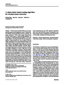
where h𝑙,𝑘 ∈ 𝑅1×𝑁 is the local observation matrix and x𝑘 ∈ 𝑅𝑁 denotes time-varying state vector which is sparse in some transform domain; that is, x𝑘 = Ψs𝑘 , where the majority of components of s𝑘 are zero and Ψ is an appropriate basis. Without loss of generality, we assume that x𝑘 itself is sparse and has at most 𝐾 nonzero components whose locations are unknown (𝐾 ≪ 𝑁). The fusion center gathers observations at all 𝑀 sensors in the 𝑀-dimensional global real-valued vector y𝑘 and preserves the global observation matrix H𝑘 = [ h𝑇1,𝑘 h𝑇2,𝑘 ⋅ ⋅ ⋅ h𝑇𝑀,𝑘 ]𝑇 ∈ 𝑅𝑀×𝑁 which satisfies the so-called restricted isometry property (RIP) imposed in the compressed sensing. Then, the global observation model can be described in (2). All the sensors are unconcerned about the sparsity. Moreover, w𝑘 and k𝑘 are uncorrelated Gaussian white noise with zero mean and covariances W𝑘 and R𝑘 , respectively. The goal of the WSN is to form an estimate of sparse signal x𝑘 at the fusion center. Due to the energy and bandwidth constraint in WSNs, the observed analog measurements need to be quantized/coded before sending them to the fusion center. Moreover, the quantized innovation scheme also can be used. At time 𝑘, the 𝑙th sensor observes a measurement 𝑦𝑙,𝑘 and computes the innovation 𝑒𝑙,𝑘 = 𝑦𝑙,𝑘 − h𝑙 x̂𝑘|𝑘−1 , where h𝑙 x̂𝑘|𝑘−1 together with the variance of innovation Cov[𝑒𝑙,𝑘 ] is received from the fusion center. Then, the innovation 𝑒𝑙,𝑘 is quantized to 𝑞𝑙,𝑘 and sent to the fusion center. As the fusion center has enough energy and enough transmission bandwidth, the data transmitted by the fusion center do not need to be quantized. The decision of which sensor is active at time 𝑘 and consequently which observation innovation 𝑒𝑙,𝑘 gets transmitted depends on the underlying scheduling algorithm. The quantized transmission of 𝑒𝑙,𝑘 also implies that 𝑞𝑙,𝑘 can be viewed as a nonlinear function of the sensor’s analog observation. The aforementioned procedure is illustrated in Figure 2.
4. A Particle Filter Algorithm with Coarsely Quantized Observations Most of the earlier works for estimation using quantized measurements concentrated upon using numerical integration
4
Mathematical Problems in Engineering variable truncated to lie in the region defined by q𝑙,0:𝑘 . So, the covariance of x𝑘 | q𝑙,0:𝑘 can be expressed as
Process xk
Cov [x𝑘 | q𝑙,0:𝑘 ] y1,k
y2,k S1
yM,k S2
···
Feedback q2,k
q1,k
SM
Feedback
Figure 2: System model.
methods to approximate the optimal state estimate and make an assumption that the conditional density is approximately Gaussian. However, this assumption does not hold for coarsely quantized measurements, as demonstrated in the following. Firstly, suppose {x𝑘 } and {𝑦𝑙,𝑘 } are jointly Gaussian; then it is well known that the probability density of x𝑛 conditioned on y𝑙,0:𝑘 is a Gaussian with the following parameters: x𝑘 | y𝑙,0:𝑘 ∼ 𝜂𝑘 + Σx𝑘 y𝑙,0:𝑘 Σ−1 y𝑙,0:𝑘 y𝑙,0:𝑘 , where 𝜂𝑘 ∼ N𝑑 (0, ⏟⏟⏟⏟⏟⏟⏟⏟⏟⏟⏟⏟⏟⏟⏟⏟⏟⏟⏟⏟⏟⏟⏟⏟⏟⏟⏟⏟⏟⏟⏟⏟⏟⏟⏟⏟⏟⏟⏟⏟⏟⏟⏟⏟⏟ Σx𝑘 − Σx𝑘 y𝑙,0:𝑘 Σ−1 y𝑙,0:𝑘 Σy𝑙,0:𝑘 x𝑘 ) ,
(12)
−1 + Σx𝑘 y𝑙,0:𝑘 Σ−1 y𝑙,0:𝑘 Cov [y𝑙,0:𝑘 | q𝑙,0:𝑘 ] Σy𝑙,0:𝑘 Σy𝑙,0:𝑘 x𝑘 .
qM,k
Fusion center
Feedback
= ΣΔx𝑘 y𝑙,0:𝑘
Under an environment of high rate quantization, it is apparent that y𝑙,0:𝑘 | q𝑙,0:𝑘 converges to y𝑙,0:𝑘 and x𝑘 | q𝑙,0:𝑘 approximates Gaussian. From Lemma 1, we note that x𝑘 | q𝑙,0:𝑘 is not Gaussian. For nonlinear and non-Gaussian signal reconstruction problems, a promising approach is particle filtering [24]. The particle filtering is based on sequential Monte Carlo methods and the optimal recursive Bayesian filtering. It uses a set of particles with associated weights to approximate the posterior distribution. As a bootstrap, the general shape of standard particle filtering is outlined below. Algorithm 0 (standard particle filtering (SPF)) 𝑖 ∼ 𝑝(x0 ) (1) Initialization. Initialize the 𝑁𝑝 particles, x0|−1 and x0|−1 = 0.
(2) At time 𝑘, using measurement 𝑞𝑙,𝑘 = 𝑄(𝑦𝑙,𝑘 ), the importance weights are calculated as follows: 𝜔𝑘𝑖 = 𝑖 𝑝(𝑞𝑙,𝑘 | x𝑘 = x𝑘|𝑘−1 , q𝑙,0:𝑘−1 ). (3) Measurement update is given by
(10)
≜ΣΔx
where y𝑙,0:𝑘 ≜ {𝑦𝑙,0 , . . . , 𝑦𝑙,𝑘 }. When {x𝑘 } and {𝑦𝑙,𝑘 } follow the linear dynamical equations defined in (9), it is well known that the covariance ΣΔx𝑘 y𝑙,0:𝑘 ≜ P𝑘|𝑘 = Cov[x𝑘 − 𝐸[x𝑘 | y𝑙,𝑘 ]] can be propagated by Riccati recursion equation of KF. Let {𝑞𝑙,𝑘 } denote the quantized measurements obtained by quantizing {𝑦𝑙,𝑘 }; that is, {𝑞𝑙,𝑘 } is a measurable function of {𝑦𝑙,0:𝑘 }. It will be shown that the probability density of x𝑘 conditioned on the quantized measurements q𝑙,0:𝑘 ≜ {𝑞𝑙,0 , . . . , 𝑞𝑙,𝑘 } has the similar characterization as (10). The result is stated in the following lemma. Lemma 1 (akin to Lemma 3.1 in [2]). The state x𝑘 conditioned on the quantized measurements q𝑙,0:𝑘 can be given by a sum of two independent random variables as follows:
where 𝜂𝑘 ∼
N𝑑 (0, ΣΔx𝑘 y𝑙,0:𝑘 ) .
(13)
𝑖=1
𝑘 y𝑙,0:𝑘
x𝑘 | q𝑙,0:𝑘 ∼ 𝜂𝑘 + Σx𝑘 y𝑙,0:𝑘 Σ−1 y𝑙,0:𝑘 [y𝑙,0:𝑘 | q𝑙,0:𝑘 ] ,
𝑁𝑝
𝑝𝑓
𝑖 x̂𝑘|𝑘 = ∑𝜔𝑘𝑖 x𝑘|𝑘−1 ,
where 𝜔𝑘𝑖 are the normalized weights; that is, 𝑗
𝜔𝑘𝑖 =
𝜔𝑘
𝑁
∑𝑖=1𝑝 𝜔𝑘𝑖
.
(14)
(4) Resample 𝑁𝑝 particles with replacement as follows. 𝑁
Generate i.i.d. random variables {𝐽𝜄 }𝜄=1𝑝 such that 𝑃(𝐽𝜄 = 𝑖) = 𝜔𝑘𝑖 : 𝐽
𝜄 = x𝑘𝜄 . x𝑘|𝑘
(15)
(5) For 𝑖 = 1, . . . , 𝑁𝑝 , predict new particles according to 𝑗
𝑖 , q𝑙,0:𝑘 ) , x𝑘+1|𝑘 ∼ 𝑝 (x𝑘+1 | x𝑘 = x𝑘|𝑘
(11)
Proof . See Appendix. It should be noted that the difference between (10) and (11) is the replacement of y𝑙,0:𝑘 by random variable y𝑙,0:𝑘 | q𝑙,0:𝑘 . Apparently, y𝑙,0:𝑘 | q𝑙,0:𝑘 is a multivariate Gaussian random
𝑗
𝑖 . i.e., x𝑘+1|𝑘 = F𝑘 x𝑘|𝑘 𝑝𝑓
(16)
𝑝𝑓
(6) Consider x̂𝑘+1|𝑘 = F𝑘 x̂𝑘|𝑘 . Also, set 𝑘 = 𝑘 + 1 and iterate from Step (2). Assume that the channel between the sensor and fusion center is rate-limited severely, and the sign of innovation ̂ 𝑙,𝑘|𝑘−1 )). scheme is employed (i.e., 𝑞𝑙,𝑘 = sign(𝑦𝑙,𝑘 − 𝑦
Mathematical Problems in Engineering
5
Obviously, the importance weights are given by 𝜔𝑘𝑖 = 𝑖 Φ(𝑞𝑙,𝑘 h𝑙 (x𝑘|𝑘−1 − x̂𝑘|𝑘−1 ); 0, R𝑒𝑘 (𝑙, 𝑙)). We note that 𝐸[x𝑘 | q𝑙,0:𝑘 ] = Σx𝑘 y𝑙,0:𝑘 Σ−1 y𝑙,0:𝑘 𝐸[y𝑙,0:𝑘 | q𝑙,0:𝑘 ]. Therefore, it will be sufficient to propagate particles that are distributed as 𝜉𝑘 | q𝑙,0:𝑘 , where
multisensor data fusion [27]. The information from different sensors can be easily fused by simply adding the information contributions to the information matrix and information state. Hence, we substitute the information form for (19) as follows:
𝜉𝑘 = Σx𝑘 y𝑙,0:𝑘 Σ−1 y𝑙,0:𝑘 y𝑙,0:𝑘 .
Y𝑘|𝑘 = Y𝑘|𝑘−1 + I𝑘
(17)
In addition, note that the quantizer output, 𝑞𝑙,𝑘 at time 𝑘, is calculated by quantizing a scalar valued function of 𝑦𝑙,𝑘 , q𝑙,0:𝑘−1 . So, on receipt of 𝑞𝑙,𝑘 and by using the previously received quantized values q𝑙,0:𝑘−1 , some Borel measurable set containing 𝑦𝑙,𝑘 , that is, 𝑦𝑙,𝑘 ∈ S𝑘,q𝑙,0:𝑘 , can be inferred at the fusion center. In order to develop a particle filter to propagate 𝜉𝑘 | q𝑙,0:𝑘 , we need to give the measurement update of the probability density 𝑝(𝜉𝑘−1 | q𝑙,0:𝑘−1 ) → 𝑝(𝜉𝑘−1 | q𝑙,0:𝑘 ) and time update of the probability density 𝑝(𝜉𝑘−1 | q𝑙,0:𝑘 ) → 𝑝(𝜉𝑘 | q𝑙,0:𝑘 ), which are described by Lemmas 2 and 3, respectively. Lemma 2. The likelihood ratio between the conditional laws of 𝜉𝑘−1 | q𝑙,0:𝑘 and 𝜉𝑘−1 | q𝑙,0:𝑘−1 is given by 𝑝 (𝜉𝑘−1 | q𝑙,0:𝑘 ) ∝ Φ (S𝑘,q𝑙,0:𝑘 ; h𝑙,𝑘 F𝑘 𝜉𝑘−1 , R𝑒𝑘 (𝑙, 𝑙)) . (18) 𝑝 (𝜉𝑘−1 | q𝑙,0:𝑘−1 ) So, if {𝜉𝑖𝑘−1|𝑘−1 }𝑖 is a set of particles distributed by the law 𝑝(𝜉𝑘−1 | q𝑙,0:𝑘−1 ), then, from Lemma 2, a new set of particles {𝜉𝜄𝑘−1|𝑘 }𝜄 can be generated. For each particle 𝜉𝑖𝑘−1|𝑘−1 , associate a weight 𝜔𝑖 = Φ(S𝑘,q𝑙,0:𝑘 ; h𝑙,𝑘 F𝑘 𝜉𝑘−1 , R𝑒𝑘 (𝑙, 𝑙)), generate i.i.d. random variables {𝐽𝜄 } such that 𝑃(𝐽𝜄 = 𝑖) ∝ 𝜔𝑖 , and set 𝐽𝜄 𝜉𝜄𝑘−1|𝑘 = 𝜉𝑘−1|𝑘−1 . This is the standard resampling technique from Steps (3) and (4) of Algorithm 0 [25]. It should be noted that this is equivalent to a measurement update since we update the conditional law 𝑝(𝜉𝑘−1 | q𝑙,0:𝑘−1 ) by receiving the new measurement 𝑞𝑙,𝑘 . Lemma 3. The random variable 𝑦𝑙,𝑘 | 𝜉𝑘−1 , q𝑙,0:𝑘 is a truncated Gaussian and its probability density function can be expressed as 𝜙(S𝑘,q𝑙,0:𝑘 ; h𝑙,𝑘 F𝑘 𝜉𝑘−1 , R𝑒𝑘 (𝑙, 𝑙)). This result should be rather obvious. Here, one can observe that 𝜉𝑘 is the MMSE estimate of the state x𝑘 given y𝑙,0:𝑘 . Since {x𝑘 } and {𝑦𝑙,𝑘 } have the state-space structure, Kalman filter can be employed to propagate 𝜉𝑘 recursively as follows: 𝜉𝑘|𝑘 = F𝑘 𝜉𝑘|𝑘−1 + K𝑘 (𝑦𝑙,𝑘 − h𝑙,𝑘 F𝑘 𝜉𝑘−1|𝑘−1 ) K𝑘 =
P𝑘|𝑘−1 h𝑇𝑙,𝑘
h𝑙,𝑘 P𝑘|𝑘−1 h𝑇𝑙,𝑘
+ R𝑘 (𝑙, 𝑙)
.
(19)
However, the information filter (IF), which utilizes the information states and the inverse of covariance rather than the states and covariance, is the algebraically equivalent form of Kalman filter. Compared with the KF, the information filter is computationally simpler and can be easily initialized with inaccurate a priori knowledge [26]. Moreover, another great advantage of the information filter is its ability to deal with
z𝑘|𝑘 = z𝑘|𝑘−1 + i𝑘 ,
(20)
where Y𝑘|𝑘 = P−1 𝑘|𝑘 and z𝑘|𝑘 = Y𝑘|𝑘 𝜉𝑘|𝑘 are the information matrix and information state, respectively. In addition, the covariance matrix and state can be recovered by using MATLAB’s leftdivide operator; that is, P𝑘|𝑘 = Y𝑘|𝑘 \ I𝑁 and 𝜉𝑘|𝑘 = Y𝑘|𝑘 \ z𝑘|𝑘 , where I𝑁 denotes an 𝑁 × 𝑁 identity matrix. The information state contribution i𝑘 and its associated information matrix I𝑘 are I𝑘 = h𝑇𝑙,𝑘 R𝑘−1 (𝑙, 𝑙) h𝑙,𝑘 i𝑘 = h𝑇𝑙,𝑘 R𝑘−1 (𝑙, 𝑙) 𝑦𝑙,𝑘 .
(21)
Together with (20), Lemma 3 completely describes the transition from 𝑝(𝜉𝑘−1 | q𝑙,0:𝑘 ) to 𝑝(𝜉𝑘 | q𝑙,0:𝑘 ). Following suit with Step (5) of Algorithm 0, suppose {𝜉𝜄𝑘−1|𝑘 }𝜄 is a set of particles distributed as 𝑝(𝜉𝑘−1 | q𝑙,0:𝑘 ); then a new set of particles {𝜉𝑖𝑘|𝑘 }𝑖 , which are distributed as 𝑝(𝜉𝑘 | q𝑙,0:𝑘 ), can be 𝑖 obtained as follows. For each 𝜉𝜄𝑘−1|𝑘 , generate {𝑦𝑙,𝑘|𝑘 } by the law described as follows: 𝑝 (𝑦𝑙,𝑘 | 𝜉𝜄𝑘−1|𝑘 , q𝑙,0:𝑘 ) = 𝜙 (S𝑘,q𝑙,0:𝑘 ; h𝑙 F𝑘 𝜉𝜄𝑘−1|𝑘 , R𝑒𝑘 (𝑙, 𝑙)) .
(22)
𝑖 . Also, set z𝑖𝑘|𝑘 = z𝜄𝑘|𝑘−1 + h𝑇𝑙,𝑘 R𝑘−1 (𝑙, 𝑙)𝑦𝑙,𝑘|𝑘
From the above, the particle filter using coarsely quantized innovation (QPF) has been derived for individual sensor. The extension of multisensor scenario will be described in Section 6.
5. Sparse Signal Recovery To ensure that the proposed quantized particle filtering scheme recovers sparsity pattern of signals, the sparsity constraints should be imposed on the fused estimate, that is, (̂x𝑘|𝑘 ). Here, we can make the sparsity constraint enforced either by reiterating pseudo-measurement update [15] or via the proposed sparse cubature point filter method. 5.1. Iterative Pseudo-Measurement Update Method. As stated in Section 2, the sparsity constraint can be imposed at each time point by bounding the ℓ1 -norm of the estimate of the state vector, ‖̂x𝑘|𝑘 ‖1 ≤ 𝜖𝑘 . This constraint is readily expressed as a fictitious measurement 0 = ‖̂x𝑘|𝑘 ‖1 − 𝜖𝑘 , where 𝜖𝑘 can be interpreted as a measurement noise [15, 28]. Now
6
Mathematical Problems in Engineering
we construct an auxiliary state-space model of the form as follows: (23)
𝑝𝑚 ̂𝜏 = where 𝛾1|1 = x̂𝑘|𝑘 and P1|1 = P𝑘|𝑘 and H [sign(̂𝛾1,𝜏|𝜏 ) ⋅ ⋅ ⋅ sign(̂𝛾𝑁,𝜏|𝜏 )], 𝜏 = 1, 2, . . . , 𝐿, 𝛾̂𝑗,𝜏|𝜏 , denotes the 𝑗th component of the least-mean-square estimate of 𝛾𝜏 (obtained via Kalman filter). Finally, we reassign x̂𝑘|𝑘 = 𝛾̂𝐿|𝐿 𝑝𝑚 and P𝑘|𝑘 = P𝐿|𝐿 , where the time-horizon of auxiliary statespace model (23) 𝐿 is chosen such that ‖̂𝛾𝐿|𝐿 − 𝛾̂𝐿−1|𝐿−1 ‖2 is below some predetermined threshold. This iterative procedure is formalized below: 𝑝𝑚 P𝜏|𝜏 sign (̂𝛾𝜏|𝜏 ) 𝛾̂𝜏|𝜏 1 , (24) 𝛾̂𝜏+1|𝜏+1 = 𝛾̂𝜏|𝜏 − 𝑇 𝑝𝑚 sign (̂𝛾𝜏|𝜏 ) P𝜏|𝜏 sign (̂𝛾𝜏|𝜏 ) + 𝑅𝜖
=
𝑝𝑚 P𝜏|𝜏
𝑇
𝑝𝑚
−
𝑝𝑚
sign (̂𝛾𝜏|𝜏 ) P𝜏|𝜏 sign (̂𝛾𝜏|𝜏 ) + 𝑅𝜖
.
(25)
5.2. Sparse Cubature Point Filter Method. Suppose a novel refinement method based on cubature Kalman filter (CKF). Compared to the iterative method described above, the resulting method is noniterative and easy to implement. It is well known that unscented Kalman filter (UKF) is broadly used to handle generalized nonlinear process and measurement models. It relies on the so-called unscented transformation to compute posterior statistics of ℏ ∈ 𝑅𝑚 that are related to x by a nonlinear transformation ℏ = f(x). It approximates the mean and the covariance of ℏ by a weighted sum of projected sigma points in the 𝑅𝑚 space. However, the suggested tuning parameter for UKF is 𝜅 = 3 − 𝑁. For a higher order system, the number of states is far more than three, so the tuning parameter 𝜅 becomes negative and may halt the operation. Recently, a more accurate filter, named cubature Kalman filter, has been proposed for nonlinear state estimation which is based on the third-degree sphericalradial cubature rule [29]. According to the cubature rule, the 2𝑁 sample points are chosen as follows: 𝜒𝑠 = x̂ + √𝑁 (Sx )𝑠 , 𝜒𝑁+𝑠 = x̂ − √𝑁 (Sx )𝑠 ,
𝜔𝑠 =
1 , 2𝑁
𝜔𝑁+𝑠 =
1 , 2𝑁
1 2𝑁 ∗ ∗𝑇 Cov [y] = ∑𝜒 𝜒 − x̂x̂𝑇 , 2𝑁 𝑠=1 𝑠 𝑠 where 𝜒∗𝑠 = f(𝜒𝑠 ), 𝑠 = 0, 1, . . . , 2𝑁.
.. . N𝑝
zk
IF
Method 1 or method 2
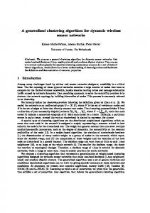
Figure 3: Illustration of the proposed reconstruction algorithm.
By the iterative PM method, it should be noted that (24) can be seen as the nonlinear evolution process during which the state gradually becomes sparse. Motivated by this, we employ CKF to implement the nonlinear refinement process. Let P𝑘|𝑘 and 𝜒𝑠,𝑘|𝑘 be the updated covariance and the 𝑖th cubature point at time 𝑘, respectively (i.e., after the measurement update). A set of sparse cubature points at time 𝑘 is thus given by 𝜒∗𝑠,𝑘|𝑘 = 𝜒𝑠,𝑘|𝑘 −
P𝑘|𝑘 sign (𝜒𝑠,𝑘|𝑘 ) 𝜒𝑠,𝑘|𝑘 1 𝑇
sign (𝜒𝑠,𝑘|𝑘 ) P𝑘|𝑘 sign (𝜒𝑠,𝑘|𝑘 ) + 𝑅̌ 𝜖
2 where 𝑅̌ 𝜖 = O (𝜒𝑠,𝑘|𝑘 2 + g𝑇P𝑘|𝑘 g) + 𝑅𝜖
,
(28)
(29)
for 𝑠 = 1, . . . , 2𝑁, where g ∈ 𝑅𝑁 is a tunable constant vector. Once the set {𝜒∗𝑠,𝑘|𝑘 }2𝑁 𝑠=1 is obtained, its sample mean and covariance can be computed by (27) directly. For readability, we defer the proof of (29) to Appendix.
6. The Algorithm (26)
where 𝑠 = 1, 2, . . . , 𝑁 and Sx ∈ 𝑅𝑁×𝑁 denotes the square-root factor of P; that is, P = Sx S𝑇x . Now, the mean and covariance of ℏ = f(x) can be computed by 1 2𝑁 ∗ 𝐸 [x] = ∑𝜒 , 2𝑁 𝑠=1 𝑠
ek
𝑝𝑚
P𝜏|𝜏 sign (̂𝛾𝜏|𝜏 ) sign (̂𝛾𝜏|𝜏 ) P𝜏|𝜏 𝑇
IF
Prediction
̂ 𝜏 𝛾 − 𝜖𝜏 , 0=H 𝜏
𝑝𝑚 P𝜏+1|𝜏+1
IF
Resample
𝛾𝜏+1 = 𝛾𝜏 ,
zk1
(27)
We now summarize the intact algorithm as follows (illustrated in Figure 3): 𝑖
(1) Initialization: at 𝑘 = 0, generate {𝜉̂0|−1 , 𝜉̂0|−1 , P0|−1 }; then compute {̂z𝑖0|−1 , ̂z0|−1 , Y0|−1 }. (2) The fusion center transmits R𝑒𝑘 (𝑙, 𝑙) which denote the (𝑙, 𝑙) entry of the innovation error covariance matrix ̂ 𝑙,𝑘 (see (31)) to (see (30)) and predicted observation 𝑦 the 𝑙th sensor: R𝑒𝑘 = H𝑘 P𝑘|𝑘−1 H𝑇𝑘 + R𝑘 , ̂ 𝑙,𝑘|𝑘−1 = h𝑙,𝑘 𝜉̂𝑘|𝑘−1 . 𝑦
(30) (31)
Mathematical Problems in Engineering
7
(3) The 𝑙th sensor computes the quantized innovation (see (32)) and transmits it to the fusion center 𝑞𝑙,𝑘 = 𝑄 (
̂ 𝑙,𝑘|𝑘−1 𝑦𝑙,𝑘 − 𝑦 R𝑒𝑘 (𝑙, 𝑙)
) R𝑒𝑘 (𝑙, 𝑙) .
(32)
(4) On receipt of quantized innovation (see (32)), the Borel 𝜎-field S𝑘,q𝑙,0:𝑘 can be inferred. Then, a set of observation particles (see (33)) and corresponding weights (see (34)) are generated by fusion center: 𝑖 𝑦𝑙,𝑘|𝑘
𝑖 ∼ 𝜙 (S𝑘,q𝑙,0:𝑘 ; h𝑙,𝑘 𝜉̂𝑘|𝑘−1 , R𝑒𝑘 (𝑙, 𝑙)) , 𝑖
𝑖 ∼ Φ (S𝑘,q𝑙,0:𝑘 ; h𝑙,𝑘 𝜉̂𝑘|𝑘−1 , R𝑒𝑘 (𝑙, 𝑙)) . 𝜔𝑙,𝑘
(33) (34)
(5) Run measurement updates in the information form 𝑖 = (see (35)) using an observation particle y𝑘|𝑘 𝑖 𝑀 𝑇 [𝑦1,𝑘|𝑘 ⋅ ⋅ ⋅ 𝑦𝑙,𝑘|𝑘 ] generated in Step (4): 𝑀
Y𝑘|𝑘 = Y𝑘|𝑘−1 + ∑h𝑇𝑙,𝑘 R𝑘−1 (𝑙, 𝑙) h𝑙,𝑘 , 𝑙=1
̂z𝑖𝑘|𝑘
=
̂z𝑖𝑘|𝑘−1
+
𝑀
∑h𝑇𝑙,𝑘 R𝑘−1 𝑙=1
(35) 𝑖 . (𝑙, 𝑙) 𝑦𝑙,𝑘|𝑘
(6) Resample the particles by using the normalized weights. (7) Compute the fused filtered estimate ̂z𝑘|𝑘 : 𝑁𝑝
̂z𝑘|𝑘 = ∑𝜔𝑖𝑘 ̂z𝑖𝑘|𝑘 ,
(36)
𝑖=1
𝑖 where 𝜔𝑖𝑘 = ∏𝑀 𝑙=1 𝜔𝑙,𝑘 .
(8) Impose the sparsity constraint on fused estimate 𝜉̂𝑘|𝑘 by either (a) or (b): (a) iterative PM update method; (b) sparse cubature point filter method. (9) Determine time updates ̂z𝑖𝑘+1|𝑘 , ̂z𝑘+1|𝑘 , Y𝑘+1|1 , 𝜉̂𝑙,𝑘+1|𝑘 , and P𝑘+1|𝑘 for the next time interval: ̂z𝑖𝑘+1|𝑘 = F𝑘 ̂z𝑖𝑘|𝑘 , ̂z𝑘+1|𝑘 = F𝑘 ̂z𝑘|𝑘 , −1
Y𝑘+1|𝑘 = [F𝑘 P𝑘|𝑘 F𝑇𝑘 + W𝑘+1 ] ,
(37)
𝜉̂𝑘+1|𝑘 = Y𝑘+1|𝑘 \ ̂z𝑘+1|𝑘 , P𝑘+1|𝑘 = Y𝑘+1|𝑘 \ I𝑁. Remarks. Here, the use of symbol 𝜉 is just for algorithm description and also can be interchanged with x. In addition, it should be noted that the proposed algorithm amounts to 𝑁𝑝 Kalman filters running in parallel that are driven by the 𝑁
𝑖 observations {𝑦𝑙,𝑘 }𝑖=1𝑝 .
6.1. Computational Complexity. The complexity of sampling Step (4) in the general algorithm is 𝑂(𝑁𝑝 ). Measurement update Step (5) is of the order 𝑂(𝑁2 𝑀)+𝑂(𝑁𝑁𝑝 ); resampling Step (7) has a complexity 𝑂(𝑁𝑝 ). Step (9) has complexity either 𝑂(𝑁2 𝐿) or 𝑂(𝑁). The complexity of time update Step (10) is 𝑂(𝑁2 𝑁𝑝 ) + 𝑂(𝑁2 𝑀).
7. Simulation Results In this section, the performance of the proposed algorithms is demonstrated by using numerical experiment, in which sparse signals are reconstructed from a series of coarsely quantized observations. Without loss of generality, we attempt to reconstruct a 10-sparse signal sequence {x𝑘 } in 𝑅256 and assume that the support set of sequence is constant. The sparse signal consists of 10 elements that behave as a random walk process. The driving white noise covariance of the elements in the support of x𝑘 is set as W𝑘 (𝑖, 𝑖) = 0.12 . This process can be described as follows: {x𝑘 (𝑖) + w𝑘 (𝑖) , if 𝑖 ∈ supp (x𝑘 ) , x𝑘+1 (𝑖) = { 0, otherwise, {
(38)
where 𝑖 ∼ 𝑈int [1, 256] and x0 (𝑖) ∼ N(0, 52 ). Both the index 𝑖 ∼ supp(x𝑘 ) and the value of x𝑘 (𝑖) are unknown. The measurement matrix H ∈ 𝑅72 × 256 consists of entries that are sampled according to N(0, 1/72). This type of matrix has been shown to satisfy the RIP with overwhelming probability for sufficiently sparse signals. The observation noise covariance is set as R𝑘 = 0.012 I72 . The other parameters are set as x̂0|−1 = 0, 𝑁𝑝 = 150, and 𝐿 = 100. There are two scenarios considered in the numerical experiment. The first one is constant support, and the second one is changing support. In the first scenario, we assume severely limited bandwidth resources and transmit 1-bit quantized innovations (i.e., sign of innovation). We compare the performance of the proposed algorithms with the scheme considered in [15], which investigates the scenario where the fusion center has full innovation (unquantized/uncoded). For convenience, we refer to the scheme in [15] as CSKF; the proposed QPF with iterative PM update method and sparse cubature point filter method are referred to as Algorithms 1 and 2, respectively. Figure 4 shows how various algorithms track the nonzero components of the signal. The CSKF algorithm performs the best since it uses full innovations. Algorithm 1 performs almost as well as the CSKF algorithm. The QPF clearly performs poorly, while Algorithm 2 performs close to Algorithm 1 gradually. Figure 5 gives a comparison of the instantaneous values of the estimates at time index 𝑘 = 100. All of three algorithms can correctly identify the nonzero components. Finally, the error performance of the algorithms is shown in Figure 6. The normalized RMSE (i.e., ‖x𝑘 − x̂𝑘 ‖2 /‖x𝑘 ‖2 ) is employed to evaluate the performance. As can be seen, Algorithm 1 performs better than Algorithm 2 and very close to the CSKF before 𝑘 = 40. However, the reconstruction accuracies of all algorithms almost coincide with each other
8
Mathematical Problems in Engineering 1
3
0
2
−1 x 27
x7
4
1
−2
0
−3
−1
0
20
40 60 Time index
80
100
−4
0
20
Algorithm 2 QPF
True CSKF Algorithm 1
40
60 Time index
100
Algorithm 2 QPF
True CSKF Algorithm 1
0.5
80
2
1.5
0
x 141
x 77
1 −0.5
0.5 −1
−1.5
0
0
20
40
60
80
100
−0.5
0
20
40
True CSKF Algorithm 1
60
80
100
Time index
Time index Algorithm 2 QPF
Algorithm 2 QPF
True CSKF Algorithm 1
Figure 4: Nonzero component tracking performance.
8
1
6
0.9 0.8 Normalized RMSE
Amplitude
4 2 0 −2 −4
0.6 0.5 0.4 0.3 0.2
−6 −8
0.7
0.1 50
True CSKF
100 150 Support index
200
Algorithm 1 Algorithm 2
Figure 5: Instantaneous values at 𝑘 = 100.
250
0
0
10
CSKF QPF
20
30
40 50 60 Time index
70
Algorithm 1 Algorithm 2
Figure 6: Normalized RMSE.
80
90
100
9
4
3
3
2
x 42
x4
Mathematical Problems in Engineering
2
0
1
0
1
0
20
40 60 Time index
80
−1
100
0
20
40 60 Time index
80
100
40 60 Time index
80
100
True Algorithm 1 Algorithm 2
True Algorithm 1 Algorithm 2 2
0.5
1.5
0
x 98
x 91
1 −0.5
0.5 −1
−1.5
0
0
20
40
60
80
100
−0.5
0
20
Time index True Algorithm 1 Algorithm 2
True Algorithm 1 Algorithm 2
Figure 7: Support change tracking.
after roughly 𝑘 = 45. It is noted that the performance is achieved with far fewer measurements than the unknowns (