IEEE TRANSACTIONS ON COMPONENTS, PACKAGING, AND MANUFACTURING TECHNOLOGY—PART C, VOL. 20, NO. 2, APRIL 1997
133
Yield Learning in Integrated Circuit Package Assembly Shankar Balasubramaniam, Abul K. Sarwar, and D. M. H. Walker, Member, IEEE
Abstract— This paper describes a yield learning model for integrated circuit package assembly. The goal was to provide a management tool for making yield projections, resource allocations, understanding operating practices, and performing what-if analyses. The model was developed using a series of case studies of packages entering manufacturing. These studies were a tape carrier package (TCP) at Intel, Chandler, AZ, a ceramic ball grid array (CBGA) and plastic quad flat pack (PQFP) at IBM, Bromont, P.Q., Canada, and a plastic ball grid array (PBGA) at Motorola, Austin, TX. These packages covered a wide range of technologies, including liquid and overmolded encapsulation, wirebond and controlled collapsed chip connection (C4) chip connections, and tape automated bonding (TAB), ceramic, laminate, and leadframe substrates. The factors that affect yield learning rates (e.g. process complexity, production volumes, personnel experience) were identified and a nonlinear spreadsheet-based response surface model was built. The model separates out the underlying chronic yield from excursions due to human error, equipment failure, etc. The model has been shown to accurately predict the yield ramp as a function of the factor values. One of the conclusions of this work is that all of the very dissimilar assembly processes had very similar factors, with very similar factor sensitivities and rankings in terms of how each affected the yield learning rate. In all cases, the most important factors were operator experience, changes in line volume, types of work teams, process complexity, equipment upgrades, and technology type. Since the yield ramp for a new product will hopefully be short, the model must be calibrated for a particular product very quickly. We have developed a graphical interface and tuning procedure so that when the production data is readily available, the tuning procedure takes only a few days. Index Terms—Defect reduction, design centering, package assembly, yield, yield learning, yield model.
I. INTRODUCTION
I
N THIS paper we examine yield learning in integrated circuit package assembly, the manufacturing process of placing bare die into packages. Package technology must keep pace with advancing integrated circuit technology, and each generation of packaging, from simple lead count increases (lead extensions) to completely new package designs carry with them manufacturing yield challenges. Today assembly yields for complex packages start high and usually mature Manuscript received March 14, 1997; revised May 8, 1997. This work was supported by the Semiconductor Research Corporation (SRC) and SEMATECH under Contract 95-PJ-804. S. Balsubramaniam and A. K. Sarwar are with Advanced System Logic, Texas Instruments, Inc., Sherman, TX 75090 USA (e-mail:
[email protected];
[email protected]). D. M. H. Walker is with the Department of Computer Science, Texas A&M University, College Station, TX 77843-3112 USA (e-mail:
[email protected]). Publisher Item Identifier S 1083-4400(97)06034-8.
above 99%. Since starting assembly yields are usually higher than mature semiconductor fabrication yields, one might think that there is no need to focus on yield learning in assembly. However since almost every assembly failure represents the loss of a good die, the economic cost of even a small amount of assembly yield loss can be very high. For example, using some recent estimates [1], a 1% assembly yield loss for the Intel Pentium microprocessor would cost $42 million annually. As a result, the mature yield and yield learning rate targets used in integrated circuit assembly are correspondingly high, and thus difficult to achieve. The integrated circuit package assembly manufacturing process follows a yield learning curve [2]. At the start of production, yields are low and attention is focused on removal of systematic problems, such as a miscentered process. Once the systematic problems are removed the yield ramp begins, and the process improvement focuses on reducing the random process variation. In process maturity the yield saturates and process improvement shifts to process control to maintain the yield at a high level. This procedure of process improvement is termed yield learning [2]. The large number of possible process disturbances, and limited process visibility make yield learning a slow and tedious process of identifying and eliminating yield detractors. The rate of yield learning is limited by the time it takes to identify a yield detractor, determine the cause, develop a solution, implement it, and verify it [2]. Yield learning is an important component of time to market since volume production cannot begin until yields have reached a profitable level. Management typically sets targets for rates of yield learning based on prior experience, and then attempts to meet them through the use of process improvement methodologies [15]. These methodologies are all based on ISO 9000 [16], and all world-class assembly factories hold an ISO 9002 certification. From the management viewpoint there are two problems with regard to yield. The first is to make accurate projections of the yield ramp in order to schedule product introduction and volume production and to estimate costs. The second is to optimize technology design, resource allocations and operating practices in order to maximize the yield learning rate. For example, would hiring more engineers improve or worsen the yield learning rate? For both problems it is infeasible to run large experiments to determine the correct decisions. Therefore a yield learning model is needed. Since as noted, the bulk of the yield learning time occurs during the yield ramp, we focus our modeling efforts on this phase of yield improvement.
1083–4400/97$10.00 1997 IEEE
134
IEEE TRANSACTIONS ON COMPONENTS, PACKAGING, AND MANUFACTURING TECHNOLOGY—PART C, VOL. 20, NO. 2, APRIL 1997
While there is a large body of research on yield learning in semiconductor manufacturing [2]–[3], there is relatively little known about yield learning in integrated circuit assembly. The literature on assembly yield focuses on process optimization and design centering, and the design of experiments (DOE) to support these activities [4]–[6]. These optimizations focus on unit process steps (e.g., wire bonding), rather than the yield of the assembly process as a whole. During the yield ramp, the process has already been centered, and the focus is on reducing process variance through process improvement and statistical quality control (SQC) techniques. Because of the lack of published data on assembly yield learning, a series of case studies were undertaken on a variety of packaging technologies entering production. We chose to study state-of-the-art technologies since these are the ones that have the most yield problems. Both technologies new to a company and lead extension projects were studied to see if the gap between new and old technology resulted in any significant qualitative or quantitative differences in yield learning. The technologies were studied from production start through most or all of the yield ramp, in order to determine how yield learning changed from the start of the ramp to process maturity. The studies done were a tape carrier package (TCP) at Intel, Chandler, AZ, a ceramic ball grid array (CBGA) and plastic quad flat pack (PQFP) at IBM, Bromont, P.Q., Canada, and a plastic ball grid array (PBGA) at Motorola, Austin, TX. These packages covered a wide range of technologies, including liquid and overmolded encapsulation, wirebond and controlled collapsed chip connection (C4) chip connections, and tape automated bonding (TAB), ceramic, laminate, and leadframe substrates. We describe our yield modeling work and results in the sections that follow. Section II describes the yield learning model and its implementation. Section III describes the model building procedure used in the case studies. Section IV describes the results of the case studies, and Section V describes conclusions and future work. II. YIELD LEARNING MODEL Yield learning can be modeled in three ways: response surface model, queuing model, and discrete event model. A response surface model (RSM) predicts the rate of yield improvement versus factor values such as production volume, process complexity, engineer experience, wire bonder power variance, etc. It has the advantage of being compact and straightforward to calibrate. A queuing model can more accurately account for effects such as reentrant flows (such as due to rework) and resource constraints. A discrete event model provides the most accuracy and detail, since it can model the real-time behavior of the manufacturing line. The disadvantage of the queuing and discrete event models is that they require a large calibration effort, and many of the required input values (e.g. engineer response time) are not readily known. It was clear from the feedback of the potential yield model user community that the rapid yield learning process in package assembly required model calibration to be done within a few days at most, and ideally in less than one day. In addition, managers are often more interested in sensitivity analysis than
they are in absolute predictions, which again suggests an RSM. As a result we chose to use a nonlinear response surface model to predict the yield ramp. The model was implemented as a Microsoft Excel spreadsheet with a Visual Basic graphical user interface and integrated tuning procedure to reduce calibration time and increase model portability and usability. There are two types of yield detractors that occur in assembly: chronic defects and excursions. Chronic defects occur repeatedly, such as bent leads, while excursions are yield drops due to random one-time events such as human error, equipment failure, etc. Due to their nature, excursions tend to result in relatively large drops in yield, such as when an entire production lot is damaged. The yield learning model predicts yield loss due to both chronic defects and excursions. The yield loss caused by chronic defects (or chronic yield) is modeled as a nonlinear response surface that is a function of factor values within each module. A module is an set of unit process steps delineated by inspection points. This delineation is necessary so that module yield can be measured. The assembly process flow consists of a sequence of modules. Examples of modules include wire bond, mold, solder ball attach, marking, etc. Modules that do not have significant yield loss, such as epoxy cure, bake out, laser marking or packing are not included in the yield learning model. Modules that are normally considered part of the assembly process, such as backgrind and wafer saw, are included in the yield model even if these steps are carried out at the wafer fab. Modules that are normally considered part of the semiconductor manufacturing process, such as wafer bumping, are not included in the model. These choices were based on operating practices in the companies studied. If a module is reused in the assembly sequence, this is incorporated in the model by replicated factor values. A factor is a variable in a module that affects the module yield learning rate. Examples include process complexity and operator experience. Only factors common to all modules are included in the model. Factors that are unique to a given module are not included. This choice was made because we are primarily interested in common factors, and view modulespecific factors (e.g. postmold cure temperature) as part of the module process optimization. A value is the value of a factor within a module. Factor values can be categorical, such as type of work team, or continuous, such as unit volume or experience. As will be described below, we have converted all continuous values that can have a wide range to categorical values. Factors are only included in the model if they can have different values between modules. For example, if all modules use visual inspection, then the yield metrology factor is not included in the model. The reason is that these common factors are incorporated into the model coefficients during the model calibration process. The chronic yield model predicts the yield slope, the average increase in yield over a work week (WW). A work week is the time unit commonly used for reporting yields. The slope prediction for each module is the average of the slope predictions for each of factors within the module, using the factor values for that work week. Note that some factors have constant value (e.g. process complexity), while other factors have values that change over time (e.g. operator experience).
BALSUBRAMANIAM et al.: YIELD LEARNING IN INTEGRATED CIRCUIT PACKAGE ASSEMBLY
The yield slope prediction for a work week is the sum of the yield slope predictions for each of modules as described in Yield Slope (1) is the value where is the slope function for factor , and for module for that work week. We found this relatively simple equation adequate to fit the production data. No cross terms were needed within or between modules. The predicted yield increase over time is then computed as the sum of the starting yield and the yield slopes for subsequent weeks. We do not attempt to model the reduction in yield slope as yield approaches 100%, but in practice just limiting the predicted yield to 100% generates realistic predictions. Each of the factor functions is implemented as a lookup table. This is possible because the factor values are categorical data (e.g. process complexity), or integer values in a small range (e.g. number of incoming materials that affect yield). As described below, continuous values that can have a wide range are converted to categories for use in factor functions. The entries in the lookup tables are termed coefficients. The coefficients are the change in yield per work week due to that value for that factor in that module. A single slope function is used in all modules for each factor. This reduces the model tuning effort, and identifies the average relationship between each factor and the overall yield learning rate. The module-to-module variations in the relationship are captured in the assignment of factor values. For example, the process complexity value for each module is assigned based on the relative difficulty in achieving a given yield slope, all other things being equal. Due to their very nature, excursions cannot be predicted, and do not appear to be related to any of our postulated factors. We theorize that the chronic yield slope must be related to the rate of excursions, in that excursions will take engineer time away from solving chronic yield problems. However there was not enough data available in our case studies to confirm this, and anecdotal evidence suggests that many excursions have an obvious cause (e.g. dropped tape reel), which does not require any engineering time to solve. For the management purposes of sensitivity analysis, what-if analysis, etc., the yield learning model only needs to consider chronic yield. However in order to provide realistic-looking yield projections, we include excursions in our model as an additional yield loss on top of the chronic yield. Excursion occurrence in each module is modeled as a Poisson process, with each occurrence causing a drop from the chronic yield level, with the drop having the same distribution as observed excursions in that module. A. Yield Model Factors The first task of the case studies was to identify the factors governing yield improvement, and assign values to them. Because of the large range of package technologies and different manufacturing plants, we expected that the factors would be different for each study. What we found was that there was a large common set of factors. In any one model, a factor might not be included due to the factory organization. For example, the Type of Teams factor is not included when
135
all work teams are dedicated to particular modules. The factors identified in the studies and their possible values are as follows. 1) Process Complexity: Nhe number of process parameters or knobs that affect the module yield. Relative ranking zero (low) to five (high). This value is fixed for the process. 2) Equipment Complexity: Number of operations performed by the equipment. Relative ranking zero (low) to five (high). This value is fixed for the process. 3) Input Complexity: Number of incoming material parameters in the module that can affect yield. This value is fixed for the process. 4) Experience Level: Experience of personnel in the module. A separate experience factor is used for each category of personnel: operators, technicians, and engineers. The number of work weeks required to achieve competence in the module is determined. The factor value is then determined by comparing the average experience of each category of personnel to this competence value and categorized into novice (average experience less than competence value), not so experienced (average experience above competence value), and very experienced (average experience at least double the competence value). The experience level changes from work week to work week depending on personnel tenure and turnover. The threshold for defining a very experienced person was based on the results of the initial case studies and a consensus of the defect reduction team. No attempt is made to derate past experience on a module in the process (e.g. when it has been some time since the person has last worked in the module). Prior experience in a similar module for another package technology is not counted. 5) Criteria: Number of times the acceptance criteria were changed during production. A change in criteria might result in units that were not rejected prior to the change to be rejected after the change for the same defect code, resulting in a yield drop. This factor accounts for a changing definition of yield. This value is fixed for the process. Hence it is more useful for sensitivity analysis than prediction. 6) Machine Additions/Upgrades: Number of equipment upgrades and additions in the module. New equipment is assumed to be more advanced, so additions and upgrades are lumped together. This value is fixed for the process. Hence it is more useful for sensitivity analysis than prediction. 7) Technology: Type of technology used in the module. The value is categorized as mechanical ( ), thermal ( ), dispense ( ), chemical ( ) or a combination of any of these. For example, wire bond is mechanical and thermal ( ), while post-mold cure is thermal. This value is fixed for the process. 8) Batching: How units are handled in a module. The value can be serial ( ), batch ( ), or a combination ( ). For example, wire bond uses serial processing, while mold is done in batches. This value is fixed for the process.
136
IEEE TRANSACTIONS ON COMPONENTS, PACKAGING, AND MANUFACTURING TECHNOLOGY—PART C, VOL. 20, NO. 2, APRIL 1997
YIELD LEARNING FACTORS
AND
TABLE I FACTOR VALUES
FOR
EXAMPLE TECHNOLOGY 1
modify it as needed, or define a new process flow. In practice most technologies can be described very quickly, and the bulk of the effort is determining the factor values. III. MODEL BUILDING PROCEDURE
9) Line Volume Changes: Change in number of units processed by the module in the work week. This value is categorized as 25% or smaller decrease, more than 25% decrease, 25% or smaller increase, and more than 25% increase in volume from the previous work week. This value changes weekly. Note that the absolute volume can vary significantly from module to module. The 25% threshold was selected based on the observed data in the initial case studies. 10) Yield Metrology: Type of yield metrology used in the module. Values can be visual inspection sampling or continuous measurement. This value is fixed for the process. 11) Type of Teams: How personnel are scheduled to work in modules. The values are dedicated ( ), i.e. they always work in a particular module, or ad hoc ( ), i.e. they are assigned to different modules as needed. This value is fixed for the process [17]. The factors and factor values used for some of the modules in one case study are shown in Table I. For proprietary reasons, the process and modules are not identified. Table II shows the significant factors and factor values for a second technology. In this case the current values for experience level are shown. In neither case is the line volume changes factor shown since its value changes weekly. B. Model Implementation The yield learning model is implemented in a Microsoft Excel spreadsheet. We chose a spreadsheet implementation so that the model would be easily portable. The model predicts the yield based on the factor values that are supplied by the user. In addition to unchanging factor values, the user also supplies the estimated start yield and weekly changes in module experience level and volume, and the desired weeks of prediction. The outputs are tables and charts of the week-by-week chronic and excursion yields, the average yield slope over the time period, and the value of final yield. In order to improve ease-of-use, a graphical user interface was implemented in Visual Basic to automate the model building and tuning procedure, and to provide simple procedures for yield prediction, sensitivity analysis, what-if analysis, etc. The process flow of the four technologies of our case studies (CBGA, PQFP, PBGA, TCP) are predefined, so that if they are relevant, the user can select one and just modify the factor values. The user can also select the predefined flows and
Each case study started with an introductory meeting to orient management and defect reduction team (DRT) engineers about the goals of the study and issues involved. This was usually followed by a line tour to orient the model-building team to the particulars of the factory and the target package technology. This was followed by an alternating series of meetings and model building activities. The following procedure was used to build the yield learning model in each case study. 1) Defect reduction engineers meet and brainstorm to identify likely factors. 2) Engineers assign values to these factors, taking into consideration issues such as the thermal and mechanical characteristics of the assembly line [6]. A consensus procedure was used to ensure the self-consistency of values within and between technologies at a company. Extending this self-consistency between companies will be discussed in Section V. 3) A factor sensitivity analysis is performed using initial production yield data to identify the most important factors. 4) Build a response surface model using the important factors, tune to initial production yield data, and check prediction accuracy. Model tuning is done by computing the factor lookup functions (coefficients) using least squares regression of the initial production yield data with the factor values. 5) Repeat steps 1-4 until all important factors are identified, and values assigned. Detailed descriptions of the model building procedure used in each case study can be found in [10]–[14]. In the first study, a total of eight hours of engineer meetings and two months of time were required to build an acceptable model. In later case studies, the set of factors and values identified in previous studies were used as a starting point. By the time of the last study, no new factors were identified, so our set of factors is sufficient for the vast majority of packaging technologies. Building a new model for a new process now takes about one day. A. Potential Factor Identification and Value Assignment Each factory uses a statistical quality control system to track manufacturing lots and inspection data. Failed units are recorded by defect code (e.g. wire bond shear test failure), with some factories having more than 1000 codes. Pareto charts are built from the data to identify the most important sources of yield loss. The corrective action taken for a particular yield problem is also recorded, so that if a problem recurs, prior solutions can be used as a reference. This problem-solution approach results in yield learning, but we found that the resulting knowledge base is not useful for building a yield learning model. For example, the set of defect codes varies
BALSUBRAMANIAM et al.: YIELD LEARNING IN INTEGRATED CIRCUIT PACKAGE ASSEMBLY
SIGNIFICANT FACTORS
AND
137
TABLE II VALUES FOR EXAMPLE TECHNOLOGY 2
widely from factory to factory. We found it essential to identify factors using a model-centric brainstorming approach. Engineer experience is required to identify potential factors and assign factor values. Identifying factors requires knowledge of parameters that affect the yield in each module. For example, the module leader knows the types of metrology used in a module. Similarly, to assign a value to a factor such as input complexity (number of incoming material parameters that affect yield) requires a good understanding of the module operation. In some processes, defective parts detected at module inspection were reworked to reduce yield loss. A common example of this is PQFP lead inspection following lead trimand-form, with units failing coplanarity specifications passing through a lead reconditioner and then through lead inspection again. In our model, parts that are successfully reworked do not count as yield loss. Consequently our model only includes factors that affect the net yield improvement caused by process improvement and successful rework. In theory, yield learning could consist entirely of improved rework yield. In practice factories try to minimize rework, so the factors identified as important to yield learning always refer to the basic process, not the rework process. B. Excursion Elimination Control charts were used to separate the chronic defects from the excursions using SQC techniques [9]. The frequency and distribution of excursions was then computed so that they could later be added to the chronic yield to compute the excursion yield. We also considered using the defect codes recorded during manufacturing to separate chronic defects and excursions. However we found that this would require significantly more effort, it would have to be customized for each factory, and it would only provide marginal improvements in the model accuracy. We were originally concerned that the small amount of training data used for prediction applications would be a problem in the presence of excursions, but we did not find this to be the case. C. Regression Analysis Least squares regression analysis in RS1, SAS, or Excel was used to estimate the coefficients for yield change for each value of the factors. Originally the analysis was done by the separate packages used at each factory, and then later this capability was put into the spreadsheet. The coefficients are the change in yield per work week due to that value for that factor, all other factors being equal. Equation (2) below depicts
Fig. 1. PQFP yield slope versus process complexity.
conceptually the estimated change in yield per work week as based upon each factor of interest Est.YieldChange
WW
(2)
, are the coefficients for the process where complexity, equipment complexity and experience level. D. Sensitivity Analysis After the yield model was built and tuned, the resulting coefficients were used to determine the sensitivity of yield to the factor values when the value is changed in all modules. It was seen that an increase in the process complexity decreased the yield slope for all the packaging technologies. Also, machine additions/upgrades and increased operator experience increased the yield slope. Fig. 1 shows the effect of process complexity on the yield slope for the PQFP. As can be seen, all but the lowest complexity level (as determined by the DRT engineers), reduces the yield slope. The case studies helped to understand the effect of each one of the factors on the learning curve for the TCP, PQFP, CBGA, and PBGA technologies. Table III shows the sensitivity of the factors on the yield slope in decreasing order of magnitude, and a possible explanation for the sensitivity. IV. CASE STUDY RESULTS Yield learning models were built for four technologies: TCP, plastic quad flat pack, ceramic ball grid array, and PBGA. The yield predictions for the chronic yield and the excursions were observed for each technology. Yield predictions made were then validated using the actual data. The validation indicated a good fit for the model, even using a limited set of training data. The process flow for each technology and corresponding yield predictions are described below. A. Tape Carrier Package (TCP) The TCP [7]–[8] is a new package designed for microprocessors in notebook computers. It has a small form factor and low weight. The package consists of a TAB tape that is bonded
138
IEEE TRANSACTIONS ON COMPONENTS, PACKAGING, AND MANUFACTURING TECHNOLOGY—PART C, VOL. 20, NO. 2, APRIL 1997
TABLE III FACTOR VALUE EFFECT ON YIELD SLOPE
Fig. 2. TCP chronic yield versus filtered actual yield.
Fig. 3. TCP excursion yield versus actual yield.
to a bumped die, with a liquid encapsulation to protect the leads and die surface. The back of the die is exposed, and directly in contact with the printed circuit board, which acts as the heat sink. The tape is singulated and shipped in coinstacked tubes. The leads are separated from the TAB frame as the package is mounted on the board. The TCP assembly process flow consists of the following major modules. 1) Wafer Bump: At the semiconductor fabrication plant, straight-wall gold bumps are placed on the die bonding pads in a liftoff process. This step is considered part of wafer fabrication and not included in the yield learning model. 2) Wafer Sort (Sort): At the semiconductor fabrication plant, each die on the wafer is electrically tested to specific pass/fail criteria. Reject die are marked with an ink dot to indicate that they should not be assembled. The wafers are then sent to the assembly plant. 3) Wafer Saw (Saw): The wafer is cut apart with a diamond saw into individual die. 4) Inner Lead Bond (ILB): Good (uninked) die are selected and the inner leads of the TAB tape are thermosonically bonded to the die bumps. 5) Singulate/Debuss/Carrier Load (SDCL): The TAB tape is singulated into individual packages, the leads are electrically isolated, and the packages are loaded into a carrier for handling. 6) Encapsulation (Encap): A protective coating is deposited on the die surface and then cured. 7) Package Marking: The package is marked with the part identification. This step does not have significant yield loss and so is not included in the model.
8) Packing: The packages are packed for shipment. This step does not have significant yield loss and so is not included in the model. The predicted chronic yield is shown in Fig. 2 for the TCP, compared to the actual yield with excursions filtered out. In this case the model is tuned retrospectively, using all the available production data. As can be seen, there are still significant variations in the filtered yield data, while the predicted chronic yield rises relatively smoothly. These features are similar for the other case studies. The reason is that the filtered yield data still contains significant random events, and our response surface model does not completely capture the effects of the detect, diagnose, solve, and validate yield learning loop. We will return to this in Section V. In all yield graphs the yield axis has been scaled and had its range adjusted for proprietary reasons. The occurrence of excursions was simulated for each module and added to the TCP chronic yield to get the excursion yield. The TCP excursion yield is then compared to the actual yield in Fig. 3. As can be seen, the predictions generally overlap except for several weeks when there were large excursions in the actual yield. B. Plastic Quad Flat Pack A standard plastic quad flat pack (PQFP) package was studied. The assembly process flow consists of the following major modules. 1) Dicing: The wafer is cut apart with a diamond saw into individual die at the semiconductor manufacturing plant. 2) Picking: Good die are picked off the wafer tape and placed on the lead frame. 3) Die Attach: The die is attached to the lead frame. 4) Wire Bond: The die bond pads are connected to the package leads using thermosonic wire bonding. 5) Molding: The die are encapsulated and the package body formed by molding with mold compound. 6) Plating: The exposed leads of the package are plated. 7) Dam Bar Cut (DBC): The packages are treated and the edges are smoothed out.
BALSUBRAMANIAM et al.: YIELD LEARNING IN INTEGRATED CIRCUIT PACKAGE ASSEMBLY
Fig. 4. PQFP chronic yield versus filtered actual yield.
139
Fig. 6. CBGA chronic yield versus filtered actual yield.
Fig. 5. PQFP excursion yield versus actual yield. Fig. 7. CBGA excursion yield versus actual yield. TABLE IV FACTOR RANKING FOR PQFP
8) Ink Mark: The package is marked with the part identification. 9) Trim Form Singulate (TFS): Packages are separated from the lead frame and leads are formed into the correct shape. 10) Packing: The packages are packed for shipment. This module is not included in the yield model since it does not have significant yield loss. Fig. 4 shows the predicted chronic yield for the PQFP versus the filtered actual yield, tuning using all production data. Fig. 5 shows the comparison between PQFP predicted excursion yield and actual yield. The model predicted the PQFP yield very accurately. This was aided by the fact that the PQFP process had relatively fewer, smaller excursions than the other case studies. Table IV shows the PQFP model factors ranked by percent of the yield learning rate contributed by each. As can be seen, operator experience and changes in line volume are most important. The same rankings with similar contributions is found in all the other case studies. C. Ceramic Ball Grid Array The ceramic ball grid array (CBGA) package provides array chip and board connect. The IBM C4 bump process is used to connect the chip to the ceramic substrate. A bypass capacitor is attached to the chip. The assembly process flow consists of the following major steps. 1) Chip Place and Clean: The die is flip chip bonded to the substrate using the IBM C4 process. Capacitors
are placed next to the chip and cleaning is done with flux. 2) Epoxy and Cure: An epoxy underfill is used to provide stress relief for the die. A thermal paste is applied to the chip to provide physical contact to the cap (lid), which is placed over the die. Epoxy cure is done in an oven at high temperature. 3) Marking and Cure: The substrate is ink marked with the part identification and the mark is cured. 4) Balling and Clean: Flux is put on the substrate, the solder balls are attached, reflowed, and then cleaned. The CBGA predicted chronic yield versus filtered actual yield are shown in Fig. 6. The yield learning model was tuned using the first four and all 19 weeks of production data, and the chronic yield curves for both are shown. The two different predictions straddle the data, indicating that a small amount of tuning data taken from the start of production can be used to predict the remainder of the yield ramp. The CBGA predicted excursion yield and actual yields are shown in Fig. 7. The predictions closely match except for a few weeks during yield excursions. The excursions in the CBGA process were relatively small. D. Plastic Ball Grid Array (PBGA) The PBGA package is based on Motorola’s MOPAC technology. It uses a laminate substrate with wirebonded die and overmolded encapsulation. The assembly process flow consists of the following major steps. 1) Scribe: The wafer is sawn into individual chips. 2) Wire Bond/Die Bond: Die are epoxy-bonded to laminate substrate strips. Die pads are connected to the substrate leads with thermosonic wire bonding. 3) Mold: The die are encapsulated by overmolding with mold compound. 4) Bump/Excise: Fluxed solder balls are attached to the laminate and reflowed. Flux is removed in a cleaning step. A hydrogen flame-off step prepares the package
140
IEEE TRANSACTIONS ON COMPONENTS, PACKAGING, AND MANUFACTURING TECHNOLOGY—PART C, VOL. 20, NO. 2, APRIL 1997
Fig. 8. PBGA chronic yield versus filtered actual yield.
Fig. 9. PBGA excursion yield versus actual yield.
surface for marking. The laminate strips are cut into individual packages. 5) Mark: The package is ink marked with the part identification and the mark is cured. The predicted chronic yield is compared to the actual filtered yield in Fig. 8, tuning using all production data. The predicted PBGA excursion yield is compared with the actual yield in Fig. 9. As can be seen, the predicted yield tracks the actual yield closely. V. CONCLUSION Rapid yield learning in integrated circuit package assembly is important to achieving low manufacturing costs and short time-to-market. Through the use of case studies, we have developed a yield learning model that applies across a wide spectrum of package technologies. This model provides management with a tool to project the yield ramp time, identify yield learning bottlenecks, and even assess the yield impact of hiring new, inexperienced personnel. The latter is particularly important in that labor turnover rates are as much as 3–5% per month in the Far East, where many assembly factories are located. Indeed, the factory with the highest assembly yields had the lowest labor turnover rate. In general management was more interested in sensitivity analysis as a means to understand the factory and guide decision making, than they were in accurate yield ramp predictions. A key learning of our work is that similar factors and factor sensitivities appear in all technologies. In all cases the most important factors were operator experience, changes in volume, types of work teams, process complexity, equipment upgrades, and technology type. The importance of operator experience and engineer experience (process complexity) confirm management intuition about the importance of personnel in yield learning. But the affect of volume changes on yield learning was counter-intuitive to managers. They all assumed that higher volumes resulted in higher yield learning rates, as in the classical manufacturing learning curve.
In assembly, sharp volume ramps overwhelm the engineers with defects, increasing the diagnosis time. In addition, the volume ramps increase cycle time, which increases the time to determine if a corrective action was effective in increasing yield. We found that the process of building the yield learning model in each case study was very helpful in providing insight to the defect reduction engineers about the relative importance of different yield learning factors, often different from their intuition. For example, intuition suggests that more extensive gowning in the clean room should improve yields. But our modeling efforts show that there is no correlation between gowning and yield, and in fact the factory with the highest yields had the least amount of gowning. Our models suggest some issues of concern for the future. The trend in assembly is to integrate several process modules together. This is most easily done in serial processes. However our models always show that batch processes have higher yield learning rates, due to the magnification of yield problems in large batches. On the other hand, our current work shows that the reduced cycle time of an integrated module increases yield learning rates. Accurate cost modeling of module integration requires yield models that handle these effects. Our current work focuses on replacing all qualitative factors (e.g. process complexity) in our yield models with quantitative metrics (e.g. number of material parameters), in order to reduce the modeling time, and to allow modeling results and experience from prior products to be applied to new products with minimal tuning. For example, the process complexity factor really combines both complexity and engineer experience. When separated out, it shows that as expected, engineer experience is the most important factor in yield learning. These more quantitative factors also show that some yield drops that we thought were excursions in fact could be explained by a change in factor values. We are also extending the model to handle the transition into maturity, where the yield learning rate falls. This is done by incorporating cycle times into the model, in particular the cycle of defect detection, diagnosis, solution implementation, and validation [2]. One goal is to be able to quantitatively decide when yield improvement activities are no longer beneficial, and operations should shift to statistical process control. In addition, the new model will account for the fact that factor sensitivities change in maturity. For example, operator experience is no longer as important, implying that new operators should be placed on mature lines, while experienced operators should be placed on new product ramps. ACKNOWLEDGMENT The authors wish to express their thanks for the mentorship of C. Alger, SEMATECH/Intel, R. Bracken, SRC, B. Connor, C. Randleman, and S. Grant, Intel, R. Schmitt and M. Dalby, IBM, and B. LaBelle, Motorola. They also wish to thank engineers too numerous to mention for contributing their time to provide data or aid in the analysis of this project.
BALSUBRAMANIAM et al.: YIELD LEARNING IN INTEGRATED CIRCUIT PACKAGE ASSEMBLY
REFERENCES [1] K. M. Thompson, “Intel and the myths of test,” IEEE Design Test Comput., pp. 79–81, 1996. [2] W. Maly, “Computer aided design for VLSI circuit manufacturability,” Proc. IEEE, vol. 78. pp. 356–392, Feb. 1990. [3] D. M. H. Walker, Yield Simulation for Integrated Circuits. Norwell, MA: Kluwer, 1987. [4] M. Sheaffer and L. Levine, “How to optimize and control the wire bonding process: Part I and Part II,” Solid State Technol., pp. 23–34, Nov. 1990. [5] T. Cheng and M. Wong, “Toward 6 sigma yield,” IEEE Trans. Comp., Hybrids, Manufact. Technol., vol. 13, pp. 112–121, June 1990. [6] S. Kumar and M. Tobin, “Design of experiment is the best way to optimize a process at minimal cost,” in Proc. IEEE Int. Electron. Manufact. Technol. Symp., Nov. 1990, pp. 166–173. [7] R. R. Tumala and E. J. Rymaszewski, Microelectronic Packaging Handbook. New York: Van Nostrand, 1989. [8] H. Xie, M. Aghazedh, W. Lui, and K. Haley, “Thermal solution to pentium processors in TCP in notebooks and sub-notebooks,” IEEE Trans. Comp., Packag., Manufact. Technol., vol. 19, pp. 54–65, Mar. 1996. [9] G. E. P. Box, Statistics for Experimenters, 1994. [10] A. K. Sarwar and D. M. H. Walker, “Yield learning model for ceramic ball grid array (CBGA) interim report,” Department of Computer Science, Texas A&M University, Tech. Rep., 1995. [11] S. Balasubramaniam and D. M. H. Walker, “Yield learning model for plastic quad flat package (PQFP) interim report,” Dept. Comput. Sci., Texas A&M Univ., College Station, Tech. Rep., 1995. [12] , “Yield learning model for tape carrier package (TCP) interim report,” Dept. Comput. Sci., Texas A&M Univ., College Station, Tech. Rep., 1995. [13] A. K. Sarwar and D. M. H. Walker, “Yield learning model for plastic ball grid array (PBGA) interim report,” Dept. Comput. Sci., Texas A&M Univ., College Station, Tech. Rep., 1995. [14] S. Balasubramaniam, A. K. Sarwar, and D. M. H. Walker, “Yield learning model for package assembly final report,” Dept. Comput. Sci., Texas A&M Univ., College Station, Tech. Rep., 1995. [15] D. Bennett et al., “SEMATECH qualification plan guidelines for engineering,” SEMATECH, Tech. Rep. 92061182A-GEN, 1992. [16] R. Rada, “ISO 9000 reflects the best in standards,” Commun. ACM, vol. 39, no. 3, pp. 17–20, Mar. 1996. [17] D. E. Bailey, “Manufacturing improvement team programs in the semiconductor industry,” IEEE Trans. Semiconduct. Manufact., vol. 10, pp. 1–10, Feb. 1997.
141
Shankar Balasubramaniam was born in Bombay, India on June 1, 1972. He received the B.S. degree in electrical engineering from the Regional Engineering College, Calicut, India, in 1993 and the M.S. degree in computer science from Texas A&M University, College Station, in 1996. He is currently employed with Texas Instruments, Sherman, TX. He was previously employed as a Research Assistant in the Department of Electrical Engineering, Indian Institute of Technology, Bombay, India. His research interests include yield modeling, statistical process control, and defect diagnosis.
Abul K. Sarwar was born in Narayanganj, Bangladesh on September 1, 1969. He received the B.S. and M.S. degrees in electrical engineering from Texas A&M University, College Station, in 1993 and 1996, respectively. He is currently employed by Texas Instruments as an Application Engineer in the Standard Linear and Logic group, Sherman, TX. His research interests include VLSI circuit and systems, logic design and verification, and yield modeling for IC packaging.
D. M. H. Walker (S’79–M’86) received the B.S. degree in engineering (with honors) from the California Institute of Technology, Pasadena, in 1979, and the M.S. and Ph.D. degrees in computer science from Carnegie Mellon University, Pittsburgh, PA, in 1984 and 1986, respectively. He is an Associate Professor in the Department of Computer Science, Texas A&M University. He was Assistant Director and Research Engineer in the SRC-CMU Research Center of Excellence for Computer-Aided Design, Department of Electrical and Computer Engineering, Carnegie Mellon University, from 1986 to 1993, and has held positions at Hughes Aircraft Company and Digital Equipment Corporation. His current research interests include integrated circuit testing, yield modeling, and design for manufacturability. Dr. Walker is a member of the Association for Computing Machinery and Sigma Xi. He was General Chair of the 1992 IEEE International Workshop on Defect and Fault Tolerance in VLSI Systems and is on the editorial board of IEEE TRANSACTIONS ON COMPUTERS.