For Shack-Hartmann wavefront sensors, these zones are generally chosen to match the lenslets, although this is not strictly necessary. Zonal reconstruction ...
Zernike vs. Zonal Matrix Iterative Wavefront Reconstructor Sophia I. Panagopoulou, PhD University of Crete Medical School Dept. of Ophthalmology
Daniel R. Neal, PhD Wavefront Sciences, Inc., 14810 Central S.E., Albuquerque, NM 87123
Abstract Purpose: Mathematical and clinical description of Zonal and Modal wavefront reconstruction. Advantages and disadvantages of each method. Conclusions: Both Modal and Zonal reconstruction can be an essential tool for evaluation of vision. Modal reconstruction generates smooth wavefront maps and provides useful metrics. Zonal Reconstruction uses the entire data set and creates very detailed maps, but doesn’t provide quantitative interpretation or intuitive visualization.
Introduction Although ocular wavefront aberrations have been measured since 1961,1 only recently, with improved aberrometers, did it become possible to routinely obtain wavefront maps under clinical conditions. In refractive surgery, apart from the long-established corneal topography, the Wavefront Analyzers are used for mapping the total aberrations of an eye through the pupil entrance. At this time, the preferred surface fitting method for characterizing the wavefront aberrations is the Zernike approximation, which uses the Zernike polynomials to describe and quantify the various wavefront surfaces. The conventional refraction can be decomposed into prism, defocus, cylinder, and axis. In the same manner, the remaining optical errors can be described with individual aberrations, so-called Zernike modes, with the process of Zernike decomposition. The evaluation of individual Zernike modes reveals large differences in their subjective impact.2,3 Studies from Applegate et al,2,3 and Williams et al,4 showed that this decomposition of the wave aberration in its fundamental components in order to approach the subjective image quality could cause misinterpretations. This occurs because Zernike modes can interact strongly with each other and not in a
-1-
simple way to determine the final image quality. Applegate et al5 have measured the interactions between different Zernike coefficients and found that pairs of aberrations can sometimes increase the acuity from each individual component, as well as lead to a larger decrease. Although the Zernike approximation is effective for describing the individual lower and higher order aberrations, they have also a smoothing effect that can significantly limit the aberrations that account for the wavefront error. Due to limitations with Zernike (modal) reconstruction, a different reconstruction method, such as zonal reconstruction, should be considered. Here we will present the concept for modal and zonal reconstructions.
Wavefront reconstruction methods The wavefront w, at any point (j,k), is related to the gradients through the vector gradient equation
∇w =
∂w ∂w i+ j = S jX, k i + S Yj , k j , ∂x ∂y
(1)
where i and j are the unit vectors in the x and y directions. Southwel (1980) 6 describes several methods for determining a wavefront surface from slope data. He describes several different geometries in common use for obtaining slope data and introduces the concept of Modal and Zonal reconstructors. In the end, the objective of either method is to take a set of wavefront gradient measurements SX and SY and calculate, or reconstruct, the wavefront map from this data.
Modal reconstructor In the modal reconstructor method, the wavefront surface is described in terms of a set of smoothly varying modes. These may be polynomials or other functions, or they may be derived from some other system properties (for example, as used in adaptive optics). The key property of these modes is that an analytic derivative can be obtained that may be fit to the measured slope data. Thus the wavefront surface may be written as
W ( x, y ) = ∑ Cn Pn ( x, y ) .
(2)
n
-2-
Since the functions Pn(x,y) are continuous and analytic through the first derivative, the wavefront gradient may be written
⎡ ∂w( x, y ) ⎤ ⎡ C ∂Pn ( x, y ) ⎤ n ⎢ ∂x ⎥ ⎢∑ ∂x ⎥ n ⎥ ⎢ ∂w( x, y ) ⎥ = ⎢ ∂P ( x, y ) ⎥ ⎢ ⎥ ⎢ ∑ Cn n ∂y ⎦⎥ ⎣⎢ ∂y ⎦⎥ ⎣⎢ n
(3)
This provides an analytic description of the wavefront slope at every point (x,y), which may be compared to the measured gradient values to obtain the appropriate set of coefficients Cn by least squares fitting or other methods. Given a set of gradient data βkx and βky at measurement point (xk,yk): A least squares fit to data may be obtained by minimizing the error function 2
M M ⎛ ⎛ ∂P ⎞ ∂P ⎞ χ = ∑ ⎜ β kx − ∑ Cn n ⎟ + ∑ ⎜⎜ β ky − ∑ Cn n ⎟⎟ ∂x ⎠ ∂y ⎠ k ⎝ n=2 k ⎝ n=2 2
2
(4)
with respect to the coefficients Cn. Once these coefficients are determined, the wavefront surface is known through Eq. 2. Eq. 4 may also be used to calculate the residual fit error, which is useful for characterizing the quality of the fit or the appropriateness of the particular set of polynomials for describing the measured data. This type of reconstructor provides a very compact notation for describing the wavefront, since the detailed shape information is contained in the modes Pn(x,y). If the modes are chosen to be polynomials that approximate physical properties, then the coefficients may be interpreted to obtain a direct description of the physical system. For example, Zernike Polynomials are often used in optics because they are closely related to the aberrations introduced in optical systems. Hence individual polynomials describe parameters such as defocus, astigmatism, coma and spherical aberration. If orthogonal polynomials are used, it is possible to separate the various effects, since the presence (or absence) of one term does not affect the others.
-3-
Zonal reconstructor The term “zonal reconstructor” comes about because, rather than describing the wavefront in terms of a set of overall modes, each of which is described analytically over the whole surface, the wavefront is described only locally over a limited zone. These zones are usually chosen to match the area described by each gradient measurement. They can represent a regular grid of square or rectangular elements or some other local region such as a hexagonal or other shape. For Shack-Hartmann wavefront sensors, these zones are generally chosen to match the lenslets, although this is not strictly necessary.
Zonal reconstruction methods There are several methods for solving for a wavefront surface that point-by-point represents a selfconsistent solution to the gradient equation (Eq. 1). These include the matrix iterative approach, direct least-square fitting for wavefront values, and spline integration. The body of this paper will concentrate on systems where the slope data was obtained on a regular set of square regions, and the average slope across each region is known. This is the typical arrangement for Shack-Hartman wavefront sensor data. The same methods can be used for other geometries, but the appropriate nomenclature would need to be developed.
Interpolating functions For Shack-Hartmann gradient data, the average slope across each lenslet is determined from focal spot position shift. Since the slope may be different for an adjacent lenslet, it is reasonable to assume an interpolating function where the wavefront slope varies linearly between lenslets. Thus
S X ( x,0) = c1 + c2 x and S Y (0, y ) = c3 + c4 y .
(5)
For a 1st order system, we will consider only those adjacent points that are either directly above or below, or right and left, of a central point. Integrating SX(x,0) and SY(0,y) along the x and y axis results in the interpolating function for the wavefront:
1 1 w( x,0) = c0 + c1 x + c2 x 2 and w(0, y ) = c0′ + c3 y + c4 y 2 . 2 2
-4-
(6)
Difference equations For a lenslet l, with center (xl,yl), the average slope over the lenslet is (SlX, SlY). It is more convenient to represent the data on a grid with indices (j,k) and spacing hx, and hy. Thus the slope data is known at points
S jX, k and S Yj , k . Evaluating Eq. 5 for adjacent points (for example, at points (j,k) and (j+1,k)) allows the determination of the coefficients:
c1 = S
X j,k
,
S jX+1, k − S jX, k
c2 =
hx
c3 = S
Y j ,k
and c4 =
S Yj , k +1 − S Yj , k hy
c0 = c0′ = w j , k .
(7)
(8)
These coefficients can be determined for each direction from the central point (j,k), i.e. (j+1,k), (j-1,k), (j,k+1), (j,k-1). This yields the following set of difference equations that describe the wavefront at a central point wjk in terms of adjacent points and the measured gradient values.
( S Yj , k −1 + S Yj , k ) = H Y+ {w j , k −1}
(9)
( S Yj , k −1 + S Yj , k ) = H Y− {w j , k +1}
(10)
w jk = w j −1, k +
hx X ( S j −1, k + S jX, k ) = H X+ {w j −1, k } 2
(11)
w jk = w j +1, k −
hx X ( S j +1, k + S jX, k ) = H X− {w j +1, k } 2
(12)
w jk = w j , k −1 +
hy
w jk = w j , k +1 −
hy
−
{
2
2
}
where H X w j +1,k is a predictor operator that predicts the wavefront of wjk from the measured slope and the values at wj+1,k.
Boundary conditions The boundary conditions must properly account for edge, corner, or interior points in the measurement. Generally, for a Shack-Hartmann or other slope sensor, there is also an independent measurement of the total amount of light that has been received by the lenslet. For a fully illuminated lenslet, this corresponds
-5-
to the total of all the pixels (above some threshold corresponding to the camera background) covered by the lenslet. For a non-rectangular measurement space, there can be an aperture that partially occludes some of the lenslet areas. Even for a circular pupil, there are a large number of edge lenslets that have a variable number of adjacent elements. Thus we define a weighting function Ijk that defines these boundaries. This function has zero value everywhere that there is no incident light. It may have a value (1) in regions where the lenslet is fully illuminated or some other intermediate value for partially illuminated lenslets.
Matrix iterative solution The weighted average of the predictions from the four different directions is given by
I j −1, k H X+ {w j −1, k }+ I j +1, k H X− {w j +1, k }+ I j , k −1H Y+ {w j , k −1}+ I j , k +1H Y− {w j , k +1}
w jk =
I j −1, k + I j +1, k + I j , k −1 + I j , k +1
.
(13)
This allows the value of the wavefront to be predicted from wavefront values in the four different directions. Gathering terms allows the definition of:
[ (
)]
[ (
)]
q jk =
hy y hx x S jk I j −1,k − I j +1,k + S jk I j ,k −1 − I j ,k +1 2 2
b jk =
h hx I j −1,k S jX−1,k − I j +1,k S jX+1,k + y I j ,k −1 S Yj ,k −1 − I j ,k +1 S Yj ,k +1 , 2 2
[
]
(14)
[
]
g jk = I j −1,k + I j +1,k + I j ,k −1 + I j ,k +1 ,
(15)
(16)
and
w j,k =
I j −1, k w j −1, k + I j +1, k w j +1, k + I j , k −1w j , k −1 + I j , k +1w j , k +1 g j,k
.
(17)
This equation allows for iterative solutions for the wavefront as given by:
w[jm, k+1] = w [j ,mk] +
(b
j,k
+ q jk )
g j,k
,
(18)
-6-
where m is the iteration number. Equation 15 contains only those points needed for an interior (uniform weighted) calculation, while the boundary conditions are contained in equation 14. An important consideration is the effect of edges on the data. For an edge or corner point, the wavefront can be predicted from only one or two directions. However, if the data is placed into a larger array that has been initialized to zero, then the intensity values at boundary points are always zero, and the boundary conditions will naturally be considered properly. It should be noted that for uniform intensity, where I=1 everywhere except at the boundaries, these equations converge to exactly the same equations as derived by Southwell.6 It generally takes a number of iterations equal to the number of lenslets across the entire array to converge to a stable solution. For laser beams or other wavefronts where the irradiance distribution varies rapidly, we have found that it is possible to replace the weighting function Ijk with the measured irradiance over each lenslet. This weighting serves to minimize the effect of increased noise as the irradiance decreases.
Examples In Figure 1, we have analyzed the same data from the measured wavefront of a human eye using both the modal and zonal methods. The modal
(a)
(b)
method (a) produces
Figure 1 – Comparison of Modal and Zonal methods for wavefront
very smooth surfaces,
reconstruction. (a) is modal reconstruction while (b) is the zonal
while much greater detail is evident in (b) the zonal method. The overall wavefront P-V was approximately the same in both cases. While the additional structure could be construed as noise, it requires a priori information to make this determination. For this case, the structure is a combination of tear film and fixed structure in the ocular wavefront measurement. In both cases, the sensor noise was low
-7-
enough not to contribute significantly to the wavefront image. Thus the structure represents a real wavefront structure, present in the measurement. In Figure 2 (a) when we look at the 10th order Zernike wavefront map there is a smoothing effect in the information, but in 2 (c) we can see a more detail map.
(a)
(b)
(c)
Figure 2 – Presentation of the higher order wavefront map of an eye 1 month after conductive keratoplasty. 2a shows the Zernike 6th order aberration map and 2c is the zonal wavefront map from the same data. 2b shows the slit lamp photo of this eye.
Discussion Zernike modes can interact with each other to determine final image quality, and the complexity of the interactions between modes means that Zernike decomposition is not really effective as a metric of subjective image quality. Modal representation has the advantage in that it can provide quantization of clinical data. In modal reconstruction, the fewer the number of Zernike orders that are used in a fit, the smoother the representation will be. On the other hand, when the data is over-smoothed, the information is mostly lost, especially for highly aberrated eyes.5
-8-
The advantage of the zonal representation is in the lack of smoothing effect due to the use of the entire raw data set, resulting in representations with higher spatial frequencies. Thus, zonal reconstruction may provide a better evaluation method for calculating customized ablation profiles in eyes dominated by higher order aberrations, as well as for diagnostic applications. Combined information from both methods could provide advantages in clinical evaluation of vision quality. Figure 3- Eye with corneal scars and the 2a and 2b represents the Zernike wavefront map of 4th and 10th order analysis respectively. 2d shows the zonal wavefront map that corresponds with the corneal topography of this eye in 2c.
Generally, zonal reconstructions lead
to a unique description of the wavefront surface at every measurement point. The zonal reconstruction supports rapid (point by point) variation in the wavefront surface and thus will provide for very highresolution wavefront description. It does not provide for a direct interpretation in optical terms. To determine defocus, astigmatism, or other parameters from zonal data requires an additional computation step. In theory, it is possible to fit very large basis sets with the modal such that the modal description can be used to describe very rapid local variations. However, for most solution methods, this would require an inordinate amount of computer computation time. The distinction between the two methods is useful to maintain, and the solution methods are generally quite different. In practice, both methods are quite useful and, with modern computers, both zonal and lower order modal may be calculated rapidly. The difference
-9-
between the wavefronts derived from the two methods may provide useful insight or interpretation of the information.
References 1.
Smirnov MS. Measurement of the wave aberration of the human eye. Biofizika 1961; 6:766:795.
2.
Applegate RA, Sarver EJ, Khemsara V.Are all aberrations equal? J Refract Surg. 2002;18 S556S562.
3.
Applegate RA, Ballentine C, Gross H, Sarver EJ, Sarver CA. Visual acuity as a function of Zernike mode and level of rms error. Optom Vis Sci. 2003; 80:97-105
4.
Williams DR. What adaptive optics can do for the eye. Review of Refractive Surgery. 2002; 3(3): 14-20
5.
Smolek MK, Klyce SD. Zernike polynomials are inadequate to represent higher order aberrations in the eye. Invest Ophthalmol Vis Sci 2003; 44:4676-4681
6.
W. H. Southwell, Wavefront estimation from wave-front slope measurements, JOSA 70(8), pp. 998–1006 (1980).
- 10 -