ZERO-TRUNCATED DISCRETE TWOPARAMETER POISSON-LINDLEY DISTRIBUTION WITH APPLICATIONS
Rama Shanker & Kamlesh Kumar Shukla
Journal of Institute of Science and Technology Volume 22, Issue 2, January 2018 ISSN: 2469-9062 (print), 2467-9240 (e)
Editors: Prof. Dr. Kumar Sapkota Prof. Dr. Armila Rajbhandari Assoc. Prof. Dr. Gopi Chandra Kaphle Mrs. Reshma Tuladhar
JIST, 22 (2): 76-85 (2018)
Published by: Institute of Science and Technology Tribhuvan University Kirtipur, Kathmandu, Nepal
JIST 2018, 22 (2): 76-85 ISSN: 2469-9062 (p), 2467-9240 (e)
© IOST, Tribhuvan University Research Article
ZERO-TRUNCATED DISCRETE TWO-PARAMETER POISSONLINDLEY DISTRIBUTION WITH APPLICATIONS Rama Shanker & Kamlesh Kumar Shukla* Department of Statistics, Eritrea Institute of Technology, Asmara, Eritrea * Corresponding E-mail:
[email protected] Received: 31 March, 2017; Revised: 25 September, 2017; Accepted: 27 September, 2017 ABSTRACT A zero-truncated discrete two-parameter Poisson-Lindley distribution (ZTDTPPLD), which includes zerotruncated Poisson-Lindley distribution (ZTPLD) as a particular case, has been introduced. The proposed distribution has been obtained by compounding size-biased Poisson distribution (SBPD) with a continuous distribution. Its raw moments and central moments have been given. The coefficients of variation, skewness, kurtosis, and index of dispersion have been obtained and their nature and behavior have been studied graphically. Maximum likelihood estimation (MLE) has been discussed for estimating its parameters. The goodness of fit of ZTDTPPLD has been discussed with some data sets and the fit shows satisfactory over zero – truncated Poisson distribution (ZTPD) and ZTPLD. Keywords: Zero-truncated distribution, Discrete two-parameter Poisson-Lindley distribution, Moments, Maximum Likelihood estimation, Goodness of fit. INTRODUCTION In probability theory, zero-truncated distributions are certain discrete distributions having support the set of positive integers. Zero-truncated distributions are suitable models for modeling data when the data to be modeled originate from a mechanism which generates data excluding zero counts.
P2 x;
P0 x; ; x 1, 2,3,... 1 P0 0;
(1.1)
Shanker et al. (2012) has obtained a discrete twoparameter Poisson-Lindley distribution (DTPPLD) defined by its probability mass function (pmf)
P0 x; ,
x 3
; x 0,1, 2,..., 0
Shanker et al. (2012) have studies the mathematical and statistical properties, estimation of parameters of DTPPLD and its applications to model count data. It should be noted that PLD is also a Poisson mixture of Lindley distribution, introduced by Lindley (1958). Shanker and Hagos (2015) have discussed the applications of PLD for modeling data from biological sciences. The DTPPLD is a Poisson mixture of a twoparameter Lindley distribution (TPLD) of Shanker et al. (2013) having probability density function (pdf)
the zero-truncated version of P0 x; can be
P1 x;
1
(1.3)
Suppose P0 x; is the original distribution. Then defined as
2 x 2
2 x 1 ; x 0,1,2,..., 0, 1 x 2
2 f1 x ; , 1 x e x ; x 0, 0,
(1.2)
(1.4)
It can be easily verified that at 1 , DTPPLD (1.2) reduces to the one parameter Poisson-Lindley distribution (PLD) introduced by Sankaran (1970) having pmf
In this paper, a ZTDTPPLD, of which zerotruncated Poisson-Lindley distribution (ZTPLD) is a particular case, has been obtained by compounding size-biased Poisson distribution 76
Rama Shanker & Kamlesh Kumar Shukla
(SBPD) with a continuous distribution. Its raw moments and central moments have been obtained and thus the expressions for coefficient of variation, skewness, kurtosis, and index of dispersion have been obtained and their nature and behavior have been discussed graphically. Maximum likelihood estimation has been discussed for estimating the parameters of ZTDTPPLD. The goodness of fit of ZTDTPPLD has also been discussed with some data sets and its fit has been compared with zero -
P3 x; ,
truncated Poisson distribution (ZTPD) and zerotruncated Poisson- Lindley distribution (ZTPLD). ZERO-TRUNCATED DISCRETE TWOPARAMETER POISSON-LINDLEY DISTRIBUTION Using (1.1) and (1.2), the pmf of zero-truncated discrete two-parameter Poisson-Lindley distribution (ZTDTPPLD) can be obtained as
x 1 2 ; x 1, 2,3,..., 0, 2 2 0 x 2 2 1
It can be easily verified that at 1 , (2.1) reduces to the pmf of ZTPLD introduced by Ghitany et al. (2008 ) having pmf
(2.1)
ZTPD while in social sciences ZTPD gives better fit than ZTPLD. The pmf of zero-truncated Poisson distribution (ZTPD) is given by
2 x 2 P4 x; 2 ; x 1, 2,3,...., 0 3 1 1 x
P5 x;
(2.2)
e x ; x 1, 2,3,...., 0 1 e x! (2.3)
Shanker et al. (2015) have done extensive study on the comparison between ZTPD and ZTPLD with respect to their applications to data sets excluding zero-counts and showed that in demography and biological sciences ZTPLD gives better fit than
To study the nature and behavior of ZTDTPPLD for varying values of parameters and , a number of graphs of the pmf of ZTDTPPLD have been drawn and presented in the figure 1.
Fig.1. Graph of the probability mass function of ZTDTPPLD for varying values of parameters α and θ. 77
Zero-Truncated Discrete Two-Parameter Poisson-Lindley ...
The ZTDTPPLD (2.1) can also be obtained from size-biased Poisson distribution (SBPD) having pmf
g x |
e x 1 ; x 1, 2,3,... , 0 x 1!
(2.4)
when the parameter of SBPD follows a continuous distribution having pdf
h ; ,
2 1 1 e ; 0, 0, 2 2 0 2 2 (2.5)
Thus, the pmf of ZTDTPPLD can be obtained as
P x; , g x | h ; , d 0
e x 1 2 2 1 1 e d x 1! 2 0
2 2 e 1 1 x 1 x 1 d 2 x 1! 0
1 x 1 1 x 2 x 1 x 2 2 x 1! 1 1
x 1 2 ; x 1, 2,3,..., 0, 2 2 0 x 2 2 1
which is the pmf of ZTDTPPLD with parameter and as given in (2.1). MOMENTS OF ZTDTPPLD The r th factorial moment about origin of ZTDTPPLD (2.1) can be obtained as
r E E X r | ; where X r X X 1 X 2 .... X r 1 .
Using (2.6), we have
r
r e x 1 2 x 1 1 e d 2 2 0 x 1 x 1 !
r 1 e x r 2 2 x 1 1 e d 2 0 x r ! xr
Taking y x r , we get
r
r 1 2 e y y r 1 1 e d 2 2 0 y! y 0
2 2 r 1 r 1 1 e d 2 0
78
(2.6)
Rama Shanker & Kamlesh Kumar Shukla
Substituting r 1, 2,3, and 4 in equation (3.1), the first four factorial moments about origin can be obtained and using the relationship between moments about origin and factorial moments about origin, the first four moments about origin of ZTDTPPLD (2.1) are obtained as
Using gamma integral and a little algebraic simplification, we get the expression for the r th factorial moment about origin of ZTDTPPLD (2.1) as
r ! 1 r 1 2
r
r 2 2
; r 1, 2,3,... (3.1)
1 2
3 4
2 1 2
2 2 2 1 2 2 1 6
2 2 2
2 1 3 2 3 2 6 3 1 24
3 2 2
2 1 4 2 7 3 6 7 6 2 24 6 1 120
4 2 2
Again using the relationship between moments about origin and moments about mean, the moments about mean of ZTDTPPLD (2.1) are obtained as
2 2
2 1 3 5 1 2 6 2 4 2 2
2 2 2
2
6 7 4 5 16 2 28 5 4 12 3 59 2 33 2 3 1 2 2 2 3 38 54 12 22 12 4 3 3 3 2 2 2
9 9 12 8 30 2 114 39 7 44 3 389 2 363 55 6 2 1 24 4 572 3 1147 2 492 36 5 308 4 1497 3 1376 2 306 9 4 3 2 3 2 2 2 3 4 686 1508 720 72 554 636 132 192 96 24 4 4 4 2 2 The coefficient of variation (C.V), coefficient of Skewness of dispersion of ZTDTPPLD (2.1) are obtained as
C.V .
1
3
5 1 2 6 2 4 2 2
1 2 79
1 , coefficient of Kurtosis 2 and index
Zero-Truncated Discrete Two-Parameter Poisson-Lindley ...
1
3 32 2
6 7 4 5 16 2 28 5 4 12 3 59 2 33 2 3 2 2 2 3 38 54 12 22 12 4 32 1 3 5 1 2 6 2 4 2 2
9 9 12 8 30 2 114 39 7 44 3 389 2 363 55 6 4 3 2 5 4 3 2 4 24 572 1147 492 36 308 1497 1376 306 9 3 2 3 2 2 2 3 4 4 686 1508 720 72 554 636 132 192 96 24 2 2 2 2 2 1 3 5 1 2 6 2 4 2 2
2 1
3 5 1 2 6 2 4 2 2 2 2 2
The nature of coefficient of variation, coefficient of skewness, coefficient of kurtosis, and index of dispersion of ZTDTPPLD (2.1) are shown graphically in figure 2.
Fig. 2. Coefficient of variation (CV), Coefficient of skewness, coefficient of kurtosis and index of dispersion plot for different values of and . 80
Rama Shanker & Kamlesh Kumar Shukla
MAXIMUM LIKELIHOOD ESTIMATION OF PARAMETERS Let
x1 , x2 ,..., xn be a random sample of size
n from the ZTDTPPLD (2.1) and let f x be the observed
frequency in the sample corresponding to X x ( x 1, 2,3,..., k ) such that
k
f x 1
x
n , where k is the
largest observed value having non-zero frequency. The likelihood function L of the ZTDTPPLD (2.1) is given by n
2 1 L 2 k 2 1 x f x x1
k
x 1
fx
x 1
The log likelihood function is thus obtained as k k 2 log L n log 2 x f log 1 f x log x 1 x x 1 2 x 1 The maximum likelihood estimates ˆ, ˆ of , of ZTDTPPLD (2.1) is the solutions of the following
log likelihood equations
k n 2 2 1 fx log L 2n nx 2 0 2 1 x 1 x 1 k n 2 1 x 1 f x log L 2 0 2 x 1 x 1
where x is the sample mean. These two log likelihood equations do not seem to be solved directly. However, the Fisher’s scoring method can be applied to solve these equations. We have
2 k fx 2 log L 2n n 2 2 1 4 2 1 nx 2 2 2 2 2 1 x1 x 1 2 2
k n 2 1 x 1 f x 2 log L 2 2 2 2 2 x1 x 1 2
2
2 k x 1 f x 2 log L n 2 2 2 1 2 log L 2 2 2 2 x1 x 1
For the maximum likelihood estimates
,
ˆ,ˆ of
where 0 and 0 are the initial values of and , respectively. These equations are solved iteratively
of ZTDTPPLD (2.1), following equations
till sufficiently close values of ˆ and ˆ are obtained. In this paper R software has been used to estimate parameters of the ZTDTPPLD.
can be solved
2 log L 2 2 log L
2 log L 2 log L 2 ˆ 0 ˆ
0
log L ˆ 0 ˆ 0 log L ˆ 0
GOODNESS OF FIT In this section, we present the goodness of fit of ZTDTPPLD, ZTPD and ZTPLD for four count data sets. The first data set is due to Finney and Varley (1955) who gave counts of number of flower having number of fly eggs. The second data set is due to Singh
ˆ 0
81
Zero-Truncated Discrete Two-Parameter Poisson-Lindley ...
and Yadav (1971) regarding the number of households having at least one migrant from households according to the number of migrants. The third data set is regarding the number of counts of sites with particles
from Immunogold data, reported by Mathews and Appleton (1993). The fourth data set is regarding the number of snowshoe hares counts captured over 7 days, reported by Keith and Meslow (1968).
Table 1: Number of flower heads with number of fly eggs, reported by Finney and Varley (1955). Number of fly eggs
Number of flowers
1 2 3 4 5 6 7 8 9
22 18 18 11 9 6 3 0 1
Total ML Estimate
88
ZTPD 15.3 21.8 20.8 14.9 8.5
Expected Frequency ZTPLD ZTDTPPLD 26.8 25.0 19.8 20.3 14.0 14.8 9.5 10.1 6.3 6.6
4.0 1.7 0.6 0.4
4.2 2.7 1.7 3.0
4.2 2.6 1.6 2.8
88.0
88.0
88.0
ˆ 2.8604
ˆ 0.7186
ˆ 0.82407 ˆ 25.41431
2
6.648
3.780
2.39
d.f. P-value
4 0.1557
4 0.4366
3 0.4955
Table 2: Number of households having at least one migrant according to the number of migrants, reported by Singh and Yadav (1971). Number of migrants
Observed frequency
1 2 3 4 5 6 7 8
375 143 49 17 2 2 1 1
Total ML Estimate
590
ZTPD 354.0 167.7 52.9
12.5 2.4 0 .4 0 .1 0.0
Expected Frequency ZTPLD ZTDTPPLD 379.0 376.4 137.2 140.2 48.4 49.0 16.7 16.5
5.7 1.9 0.6 0.5
5.3 1.7 0.6 0.3
590.0
590.0
590.0
ˆ 0.9475
ˆ 2.2848
ˆ 2.56082 ˆ 3.33174
2
8.922
1.138
0.51
d.f. P-value
2 0.0115
3 0.7679
2 0.7749
82
Rama Shanker & Kamlesh Kumar Shukla
Table 3: The number of counts of sites with particles from Immunogold data, reported by Mathews and Appleton (1993) Number of sites with particles
Observed frequency
Expected Frequency ZTPD
ZTPLD
ZTDTPPLD
1
122
115.8
124.7
123.0
2
50
57.4
46.7
48.7
3
18
18.9
17.0
17.5
4 5
4 4
4.7 5.9
6.1 3.5
5.9 2.9
Total
198
198.0
198.0
198.0
ML Estimate
ˆ 0.9906
ˆ 2.1831
ˆ 2.65049 ˆ 15.23738
2
2.140
0.617
0.11
d.f.
2
2
1
P-value
0.3430
0.7345
0.7401
Table 4: The number of snowshoe hares counts captured over 7 days, reported by Keith and Meslow (1968) Number of times hares caught
Observed frequency
Expected Frequency ZTPD
ZTPLD
ZTDTPPLD
1
184
174.6
182.6
183.1
2
55
66.0
55.3
54.6
3 4 5
14 4 4
16.6 3.2 0.6
16.4
16.3
4 .8 1 .9
4.8 2.2
Total
261
261.0
261.0
261.0
ML Estimate
ˆ 0.7563
ˆ 2.8639
ˆ 2.35111 ˆ 0.000236
2
2.464
0.615
0.46
d.f.
1
2
1
P-value
0.1165
0.7353
0.4976
It is obvious from the goodness of fit of ZTDTPPLD, ZTPD, and ZTPLD that ZTDTPPLD gives better fit in tables 1, 2 and 3, while in table 4 ZTPLD gives better fit. The nature of the
probability mass functions of the fitted distributions, ZTDTPPLD, ZTPLD, and ZTPD for four data sets has been shown graphically in the figure 3. 83
Zero-Truncated Discrete Two-Parameter Poisson-Lindley ...
Fig. 3. Probability plots of ZTDTPPLD, ZTPLD and ZTPD for fitted data sets in table 1, 2, 3, and 4. CONCLUSIONS In this paper, a zero-truncated discrete twoparameter Poisson-Lindley distribution (ZTDTPPLD), of which zero-truncated PoissonLindley distribution (ZTPLD) is a particular case, has been derived by compounding size-biased Poisson distribution (SBPD) with a continuous distribution. Its moments, and moments based measures including coefficient of variation, skewness, kurtosis, and index of dispersion have been obtained and their nature and behavior have been studied graphically. Maximum likelihood estimation has been discussed for estimating the parameters of ZTDTPPLD and the goodness of fit has been discussed with four data sets and in majority of data sets ZTDTPPLD shows quite satisfactory fit over ZTPD and ZTPLD.
REFERENCES Finney, D. J. and Varley, G. C. (1955). An example of the truncated Poisson distribution. Biometrics, 11: 387–394. Ghitany, M. E.; Atieh, B. and Nadarajah, S. (2008 a). Lindley distribution and Its Applications, Mathematics Computation and Simulation, 78: 493-506. Ghitany, M. E.; Al-Mutairi, D. K. and Nadarajah, S. (2008b). Zero-truncated Poisson-Lindley distribution and its Applications. Mathematics and Computers in Simulation, 79 (3): 279–287. Keith, L. B. and Meslow, E. C. (1968). Trap response by snowshoe hares. Journal of Wildlife Management, 32: 795–801. Lindley, D. V. (1958). Fiducial distributions and Bayes’ Theorem. Journal of the Royal Statistical Society, Series B, 20: 102–107. Mathews, J. N. S. and Appleton, D. R. (1993). An application of the Truncated Poisson Distribution to Immunogold Assay. Biometrics, 49: 617 – 621
ACKNOWLEDGEMENTS Authors are grateful to the Editor-In-Chief of the Journal and the anonymous reviewer for constructive suggestions which improved the quality and the presentation of the paper. 84
Rama Shanker & Kamlesh Kumar Shukla
Sankaran, M. (1970). The discrete Poisson-Lindley distribution. Biometrics, 26: 145-149. Shanker, R.; Sharma, S. and Shanker, R. (2012). A Discrete Two Parameter Poisson Lindley Distribution. Journal of Ethiopian Statistical Association, 21: 22 - 29. Shanker, R.; Sharma, S. and Shanker, R. (2013). A Two Parameter Lindley Distribution for Modeling Waiting and Survival Times Data. Applied Mathematics, 4 (2): 363 - 368 Shanker, R. and Hagos, F. (2015). On PoissonLindley distribution and Its Applications to
Biological Sciences. Biometrics & Biostatistics International Journal, 2 (4): 1-5. Shanker, R.; Hagos, F.; Sujatha, S. and Abrehe, Y. (2015). On Zero-truncation of Poisson and Poisson-Lindley distributions and Their Applications. Biometrics & Biostatistics International Journal, 2 (6): 1-14. Singh, S. N. and Yadav, R. C. (1971). Trends in rural out-migration at household level, Rural Demography, 8: 53-61.
85