028 - Forecasting Dutch GDP using large Scale Factor Models (PDF

DNB Working Paper No. 28/February 2005

DNB W O R K I N G P A P E R

Ard H.J. den Reijer

Forecasting dutch gdp using large scale factor models

De Nederlandsche Bank

Forecasting dutch GDP using large scale factor models

Ard H.J. den Reijer *

* Views expressed are those of the individual author and do not neccessarily reflect official positions of De Nederlandsche Bank.

Working Paper No. 028/2005 February 2005

De Nederlandsche Bank NV P.O. Box 98 1000 AB AMSTERDAM The Netherlands

Forecasting Dutch GDP using Large Scale Factor Models Ard H.J. den Reijery

Februari 2005

Abstract This paper applies large scale factor models to Dutch quarterly data in order to generate forecasts of GDP growth rates for an horizon up to 8 quarters ahead. The data set consists of the series underlying the central bank ´ s macroeconomic structural model for the Netherlands supplemented with leading indicator variables. In a pseudo out-of-sample forecasting context, we select optimal models in the time dimension and the optimal size of the ordered data set in the cross-sectional dimension. The main empirical …ndings of this paper are that the cross-sectional optimization substantially improves the forecasting performance of the factor models. However, only the dynamic factor model systematically outperforms and encompasses the autoregressive benchmark model with an optimal subset of the data of around 110 series. The forecasting gains in terms of mean squared errors range from 10% to 30% for forecast horizons up to 6 quarters ahead.

Keywords: Factor models, Forecasting, Leading Indicators.

JEL Code: C43, C51, E32

The author would like to thank Peter Kugler for his introduction of factor models at the Oesterreichische Nationalbank workshop, Claudia Kerkho¤ for extensive statistical assistance and seminar participants at DNB, Lex Hoogduin, Franz Palm and Peter Vlaar for comments and guidance. The views expressed in this article are those of the author and do not necessarily represent those of De Nederlandsche Bank or the European System of Central Banks. y Research Division, De Nederlandsche Bank, P.O. Box 98, 1000 AB Amsterdam, The Netherlands, tel: +31 20 5243845, fax: +31 20 5242529, e-mail [email protected]

1

1

Introduction

Empirical research on forecasting macroeconomic key variables aims to provide …scal and monetary policymakers with the most accurate predictions. The univariate and low order VAR models are currently the standard small-scale models for practical short term macroeconomic forecasting. These models include only a small number of variables while policymakers and applied forecasters are keen to extract information from many more series describing economic activity at a more disaggregate level. The increase in the quantitity and quality of readily available economic data stimulates a direction in macroeconometric research that explicitly incorporates information from a large number of macroeconomic variables into formal statistical models. The underlying idea behind this direction is the implicit assumption that the essential characteristics of macroeconomic motions are captured by a few driving aggregate forces and that the information contained in all potentially available economic key variables at an aggregate level are individually less informative about macroeconomic behaviour. This paper applies the large scale factor models proposed by Stock and Watson (2002a) and Forni et al. (2000) to Dutch quarterly data to forecast GDP growth rates for an horizon up to 8 quarters ahead. The data set of 370 series consists of the series underlying the central bank ´s macroeconomic structural model for the Netherlands supplemented with leading indicator variables. Examples of the growing empirical forecasting literature dealing with factor models include on Austrian data, Schneider and Spitzer (2004), on Belgian data, Nieuwenhuyze (2004), on euro area data, Altissimo et al. (2001), Angelini et al. (2001), Marcellino et al. (2003), on French data, Bruneau et al. (2003), on German data, Dreger and Schumacher (2002), on UK data, Artis et al. (2002) and on US data Stock and Watson (2002b). The empirical literature suggest that factor-based forecasts tend to outperform small-scale rival models, although the evidence is not overwhelming, see for instance Banerjee et al. (2003). Although factor models are designed to handle large sets of data, Boivin and Ng (2003) show in a more recent paper that extending a data set not necessarily improves the forecasting performance if the additional series are noisy or unrelated to the target variable. This paper is organised as follows. Section 2 gives an overview of factor models and starts with a brief historical sketch of the development of factor models. The subsequent subsections present the factor model speci…cation and highlight the essential di¤erences between the static and the dynamic approaches. Section 3 brie‡y describes the construction of the Dutch data set. A full description can be found in the appendix. Section 4 sets up the empirical forecasting exercise. In the subsections we perform the exercise on the full data set and we subsequently optimize the forecasting performance across the cross-sectional dimension of the data set. Finally, section 5 concludes.

2

2

The factor model

Pioneering contributions to empirical business cycle research were Mitchell and Burns (1938) and Burns and Mitchell (1946). They proposed to analyze the business cycle by taking contemporaneous averages of all the indicator series, which summarized their data set into a single index. Their practices have become widely applied. For example, the indexes of leading and coincident indicators originally developed at the National Bureau of Economic Research (NBER), which still attract considerable attention as useful tools for predicting future economic conditions. The basic notion that business cycles represent comovements in a set of series was formalized for instance by Stock and Watson (1989). They estimate the index of economic activity as the unobservable factor in a dynamic factor model for four coincident indicators: industrial production, real disposable income, hours of work and sales. Generally, factor models form a formal representation of index models by assuming that the data is driven by a few common factors thereby dramatically reducing the dimension of the data set with as little loss of information as possible. The factors capture the dynamic common variation contained in the data set. Within the factor model structure, the motion of each variable can be decomposed into two mutually orthogonal components: a common component, which is a linear combination of the common factors and therefore strongly correlated with the panel and an idiosyncratic component. This latter component contains the remaining variable speci…c information and is only weakly correlated across the panel. The di¤erent types of factor models di¤er according to the properties of the common and the idiosyncratic components. The classical, or exact factor model assumes that the idiosyncratic components of distinct cross-sectional items are mutually orthogonal. This type of factor model is typically applied in a social sciences context where one wants to quantify a variable for which no measuring instrument exists, for example quality of life, hapiness or general intelligence. The approximate factor model of Chamberlain and Rothschild (1983) and Connor and Korajczyk (1988), or generalized static factor model, drops the mutual orthogonality assumption and allows for some mild cross-correlation amongst the idiosyncratic processes. These models are typically applied in …nancial econometrics, Arbitrage Pricing Theory (APT), but potentially also in macroeconomics when the object of study is the transmission mechanism of regional or sectoral speci…c shocks. Another improvement of the classical factor model is the introduction of dynamic interrelationships of the variables by the dynamic factor model, Sargent and Sims (1977) and Geweke (1977). This model is dynamic since the common factors can hit the series at di¤erent times, although the mutual orthogonality assumption on the idiosyncratic components is maintained. So, the covariation among the observable variables is due entirely to the covariation of their common components driven by the common factors. The variation of an individual variable is due to the variation of its idiosyncratic component as well as the variation and covariation of its common component. In the more recent literature on factor models, Stock and Watson (2002a) and Stock and Watson (2002b) introduced dynamics into the approximate static factor model. By as3

suming that the common factors hit the variables only up to a …nite lag, the dynamics are represented by including lagged factors in the model speci…cation. The main advantage of this static representation of the dynamic factor model lies within the estimation techniques. The static factors in the generalized static (representation of the dynamic) factor model can be estimated by static principal components, see Connor and Korajczyk (1988), which is an eigenvalue decomposition of the contemporaneous covariance matrix. The estimated factors e¤ectively summarize the contemporaneous cross-sectional information of n variables into a limited amount of, say, r common factors with r typically small with respect to n: r n. The Generalized Dynamic Factor Model (GDFM) as outlined in Forni et al. (2000), Forni et al. (2004) and Forni and Lippi (2001) basically exploits the dynamic structure of the data by estimating the factors as the dynamic principal components of the dynamic covariation matrix, i.e. the spectral density matrix. The estimated factors e¤ectively summarize the crosssectional dimension of n variables shifted through time into a limited amount of, say, q common dynamic factors and q r. So, the factor model is dynamic when the di¤erent variables are hit by di¤erent lags of the common factors, while it is static when all variables are hit by the common factors at the same time. The dynamics of the model are a desirable feature since macroeconomic variables in general are non-synchronized and leading indicators should especially in a forecasting context play a crucial role. Moreover, the GDFM measures the lead/lag relationships between the variables allowing them to be classi…ed as lagging, coincident and leading with respect to the business cycle, see for instance Altissimo et al. (2001) for the euro area coincident business cycle indicator eurocoin. Inklaar et al. (2004) creates an alternative euro area indicator by applying the GDFM to a carefully preselected data set, which makes it then feasible to quantify the contribution of each ividual variable to the index.

2.1

The model

Consider a panel of observations xTn consisting of T observations for n time series, which are realisations of real-valued zero-mean stationary stochastic processes x =nfxit ; i 2 N; t 2 Zg indexed o N Z where the n-dimensional vec0 tor processes xnt = (x1t :::xnt ) ; t 2 Z ; n 2 N are stationary, with zero mean and …nite second-order moments. Stationarity is achieved by suitable transformations of the raw data, see the Appendix for details. In factor models, the vector of n time series is represented as the sum of two mutually orthogonal unobservable components, a common component driven by a small number of common shocks or factors a¤ecting all the variables in the data set and an idiosyncratic component related to speci…c shocks a¤ecting only a limited number of variables. So, each observation xit is the sum of the unobserved common component it and the unobserved idiosyncratic component it : The common components are driven by a q-dimensional vector of common dynamic factors ut = (u1t :::uqt ), with q independent of n and in empirical applications typically small with respect to n: q n. The vector of common shocks ut is a

4

q-dimensional orthonormal white noise process. De…ning 0 nt = ( 1t ::: nt ) , the factor model reads as xnt = Bn (L) [A (L)]

1

ut +

nt

=

nt

+

nt

=

nt

n Ft

= (

+

nt

0

1t ::: nt )

;

(1)

where the dynamic loadings are represented by a (n q)-polynomial of or0 der s : Bn (L) = (bi1 (L) ; :::; biq (L)) = Bn0 + Bn1 L + ::: + Bns Ls with L standing for the lag operator. The VARMA(S; s) transfer function A (L) is an invertible (q q)-polynomial of order S s + 1 independent of the size of the crosssection n. The …rst part of equation (1) is the generalized dynamic factor model (GDFM) of …nite order s. The latter part of the representation is simply 0 1 obtained by letting Ft = ft0 ft0 1 :::f 0t s with ft := (f1;t :::fq;t ) for [A (L)] ut and n = (Bn0 Bn1 ::: Bns ) involving r = q (s + 1) common static factors loaded only contemporaneously. So, for instance ft and ft 1 are two distinc static factors, but can be di¤erent lags of the same dynamic factor. The dynamic nature of (1) implies that Ft has a special structure: indeed, if s > 0 the rank of the spectral density matrix of Ft (namely q) is smaller than the rank of the covariance matrix of Ft (namely r). The underying assumptions determine the speci…c form of the factor model. In the static factor model interpretation of (1), the matrix Ft is an (T r)-matrix of r unobservable common shocks and N ) matrix of factor loadings, which determine the impact of comn the (r mon shock r on series n. In the dynamic factor model interpretation of (1), the (T q)- matrix u of common shocks is a q-dimensional unobservable orthonormal white noise process and the dynamic factor loadings are Bn (L) : Generally, normalization is assumed in the canonical static factor model, V ar (F) = Ir ; but (1) potentially allows for autocorrelated factors. It should be noted that the common unobserved factors are only de…ned up to a linear transformation in every factor model speci…cation. For instance, it is always possible to premultiply F by a non-singular r r-matrix Q which results in observationally equivalent factors and factor loadings: F = QQ 1 F = F ; so that F and are de…ned up to a rotation matrix. This lack of identi…cation is not a problem in a forecasting context since we are interested in the part of the time series ‡uctuations explained by all the common factors and not in the common factors separately. However, the issue of identi…cation (or rotation) should be taken into consideration when interpreting the factors in a structural way. The interpretation of the factors is ultimately a question of empirical modelling. In empirical …nance applications of asset pricing, this issue is dealt with using observable factors and putting a speci…c structure on the loadings matrix and ordering the data accordingly. A di¤erent way used by Forni et al. (2003) is to apply the identi…cation strategy for structural VARs in an appropriate format to factor models. Moreover, we de…ne the following quantities. Let n ( ) = n ( )+ n ( ) ; 2 [ ; ] ; be the spectral density matrices of xnt = nt + nt respectively, and nk ( ) ; pnk ( ) = (pnk;1 ( ) :::pnk;n ( )) the k-th largest dynamic eigenvalues and corresponding dynamic eigenvectors respectively, namely the mappings ! nk ( ) and ! pnk ( ). Denote by nk ( ) ; nk ( ) the k-th largest 5

dynamic eigenvalues corresponding to n ( ) ; n ( ) respectively. Let nh = nh + nh be the h-lag covariance matrices of xnt = nt + nt respectively, and nk ; Snk the k-th largest static eigenvalues and corresponding static eigenvectors respectively of n0 : Denote by nk ; nk the k-th eigenvalues of n0; n0; respectively. The standard assumption underlying all factor models is the orthogonality between nt and nt : FM1 The process ut is orthogonal to

it ,

i = 1; :::; n; t 2 Z:

Moreover, factor models di¤er according to their assumptions on the idiosyncratic components. FM2

a the canonical static and dynamic factor model model E 0 if t 6= or i 6= j ; diag (d1 ; :::; dn ) otherwise

0 it j

=

b the generalized static and dynamic factor model: there exists a real such that n1 respectively n1 ( ) for any 2 [ ; ] and any n 2 N: Note that condition FM2b includes and relaxes condition FM2a, by allowing for a limited amount of cross-correlation among the idiosyncratic components. Moreover, FM3

a the generalized dynamic factor model: a.e. in [ ; ] ;

nq

( ) ! 1 as n ! 1,

b static representation of the dynamic factor model: limn!1 where r := q (s + 1) :

nr

= 1,

Note that condition FM3 ensures a minimum amount of cross-correlation between the common components and implies that each ujt is present in in…nitely many cross-sectional units with non-decreasing importance. Under the assumptions, the common and the idiosyncratic components are asymptotically identi…ed when (n; T ) ! 1 and can be consistently estimated, see Forni and Lippi (2001). Note that FM3b rules out the case in which some of the elements ft k ; k = 0; :::; s are loaded only by a …nite number of the x´s and so is a stronger assumption than FM3a. For example, if 1t = ut 1 and it = ut for i 2, FM3a holds with q = 1, but FM3b does not hold since n1 ! 1 whereas n2 :remains bounded as n ! 1:

2.2

One-sided estimation and forecasting

Since the common dynamic factors ut and the common static factors Ft are latent, they need to be estimated. Given that n is …xed and much smaller than T; the factor model can be estimated by maximum likelihood. As n grows the number of parameters to be estimated becomes large and the computations involved 6

cumbersome. In a data-rich macroeconomic environment where the number of cross sections n can be larger than the number of time periods T , potential information is lost when limiting the number of cross-sections in order to ful…ll the assumptions. For instance, the likelihood function of the multivariate model requires the sample covariance matrix. The rank of sample covariance matrix does not exceed min fn; T g, wheras the rank of population covariance matrix can always be n. In order to deal with a large data set, the non-parametric principal component estimator is introduced by Connor and Korajczyk (1988) for …nance application, by Stock and Watson (2002a) and re…ned by Forni et al. (2000) for macroeconomic applications. The (dynamic) principal components can be obtained by the eigenvector and eigenvalue decomposition of the cross-correlation matrix or, in case of dynamic principal components, the spectral density matrix. The underlying idea is that idiosyncratic causes of variation, although possibly shared by many units, are poorly correlated and cancel out by averaging along the cross-section of the (synchronized) data whereas the common sources of variation do not. Hence, the literature shows that the factor space spanned by the common factors and the approximate factor space spanned by the principal components coincide when n ! 1: The common components are then obtained by projecting the data on the (past, future and) present values of the (dynamic) principal components corresponding with the diverging eigenvalues, see FM3: nt 0

0

e n ( ) pn ( ) xnt = Sn Sn xnt = p

with Sn = (Sn1 :::Snr ) the (r 0

(2)

n) matrix of static eigenvectors and pn ( ) =

(pn1 ( ) :::pnq ( )) the (q n) matrix of dynamic eigenvectors as a function of the frequency : Tilde denotes conjugate and transpose. The dynamic eigenvectors can be translated into a time domain …lter by the inverse discrete Fourier transform: " # 1 R 1 P ik pn (L) = pn ( ) e d Lk : (3) 2 k= 1 Equation (3) shows that in the dynamic case time …lters are applied to the x´s in addition to averaging along the cross-sections. The dynamic method synchronizes the data in the time dimension in order to maximize the common variation relative to the idiosyncratic variation of each variable. The idiosyncratic variation consequently cancels out more e¢ ciently by averaging along the cross-sectional dimension. As orthogonal projections of the data on the principal components, equation (2) shows that the common component is a linear combination of the data. The common components ´s in the dynamic factor model are loaded on the past, present and future values of the dynamic factors and are two-sided …lters of the data. The two-sidedness of the dynamic method creates a problem at the end of the sample when we estimate the model with a …nite panel of observations xTnt : Given the sample of T observations, denote by Tn ( ) a consistent periodogram-smoothing or lag-window estimator of the spectral density n ( ) : Moreover, denote all …nite sample estimators of 7

the population quantities by adding a superscript T . The common component estimator Tnt of (2) as a two-sided …lter deteriorates as t approaches T . For this reason, the estimator can not be used for prediction. A two-step, onesided estimator has been therefore proposed in Forni et al. (2002) which aims at constructing a one-sided …lter while maintaining the advantage of the dynamic method. The basic idea is that the estimates of the contemporeanous covariance matrix of the common components, n0T provide a better approximation of the factor space, which can be exploited to obtain in a second step a one-sided …lter. T T nk is the k-lag covariance matrix of nt and is the inverse Fourier transform T of the corresponding spectral density matrix n ( ) : T

nk

=

Z

eik

P

T

n

( )d

(4)

T

Now, n0 may produce a better approximation of the factor space while all the idiosyncratic movement is …ltered out by the dynamic method. In the T second step, n0 will be used to obtain one-sided averages of the x´s which minimizes the fraction of idiosyncratic variance contained in the aggregates and mitigates the di¢ culties at the end of the sample. Formally, in the second step jT we want to …nd r linear combinations Wnt = ZTnj xnt , where the weights ZTnj are de…ned recursively as follows: ZTnj

=

T 0 n0 a

arg maxn a

subject to

a a

a2R T 0 n0 a = T T0 n0 Znm

(5)

1 = 0 for 1

m

j

1

for j = 1; :::; r, a prime denoting transpose (for j=1 only the …rst constraint applies). The vector ZTnj turns out to be a generalized eigenvector of the couple of matrices

T n0 ;

T n0

jT and the linear combinations Wnt are the generalized principal

components of xTnt . Now, the forecast h periods ahead for the common component of variable i based on information available at time T , nT i;T +hjT is the jT orthogonal projection of xn;T +h on the space spanned by the r aggregates WnT ; j = 1; :::; r, i.e: nT i;T +hjT

T T nh Zn

= 0

ZTn

0

0

T T n0 Zn

1

0

ZTn xTnT ;

(6)

for i = 1:::n and ZTn = ZTn1 :::ZTnr : Forni et al. (2002) prove the consistency of estimator (6). Moreover, they show that computing generalized principal components of xnt is equivalent to computing the standard principal compoT nents of ynt = HxTnt = H Tnt + H Tnt ; where H is a speci…c normalization such that H nt is the (n n)-identity matrix. In case of a diagonal idiosyncratic coT ; the transformation amounts to dividing each variable xTit variance matrix n0 8

by the standard deviation op the its idiosyncratic component. The estimator in the second step weighs down noisy data, which are the variables possessing low common-to-idiosyncratic variance ratios. To sum up, the dynamic factor approach exploits two features of the data: i) sizable di¤erences in commonto-idiosyncratic variance ratios and ii) substantial heterogeneity, among crosssectional units, in the lag structure of the factor loadings. Concerning this latter feature, the dynamic factors describe the dynamic structure of the data more parsimoniously and should therefore result in less cross-sectional and serial correlation amongst the idiosyncratic components. Given the data set, the dynamic approach more easily ful…lls condition FM2b. Using the static factor model approach, Boivin and Ng (2003) show that the two features of the data resulting in the dispersion of the importance of the common component and the amount of cross- and serial-correlation among the idiosyncratic components hamper the precision of the estimates and the forecasting performance.

2.3

Estimation and speci…cation of the dynamic factor model

The frequency domain techniques require a …nite approximation of the in…nite T interval 2 [ ; ] : Let the spectral density matrix Tn ( ) = ij ( ) ; 2 [ ; ] of xnt be a consistent periodogram-smoothing or lag-window estimator of the spectral density n ( ) = ( ij ( )) of xnt calculated on a discrete grid h PT

( h) =

n

M X

T ik nk !k e

h

;

h

= 2 h= (2M + 1) ;

h = 0; :::; 2M (7)

k= M

1 PT where Tnk = (n k) t=k+1 xnt xn;t k is the sample covariance matrix and !k = 1 k= (M + 1) the Bartlett lag window of size M , which diverges whereas M=T tends to zero at some rate. We set M (T ) = round 2T (1=3) so that as in Forni et al. (2000) the convergence rate is M (T ) = O T (1=3) : The estimators of the dynamic eigenvectors pTn ( h ) are used to obtain the common T

components in (2). The estimator of the spectral density matrices n ( ) is the projection of the …rst q principal components weighted by their corresponding eigenvalues on the …nite grid h : P

n

T

( h) =

T n1

( h) p ~ Tn1 ( h ) pTn1 ( h ) + ::: + T

T nq

( h) p ~ Tnq ( h ) pTnq ( h )

(8)

Its discrete equivalents n ( h ) is straightforwardly de…ned by replacing the dynamic eigenvalues and eigenvectors in (8) by their equivalents based on the …nite grid h : In addition to the determination of the size of the lag window for Fourier transformations, the number of common factors q has to be chosen. Concerning the number of static factors r; Bai and Ng (2002) derive information criteria 9

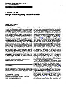
to determine the optimal number as a trade-o¤ between the goodness-of-…t and over…tting. The information criteria are extensions of the familiar Akaike, Schwarz and Bayes criteria by including the cross-section dimension n in the penalty function of over…tting.We will use the average of the results of the two best performing information criteria termed ICp1 and ICp2. The Bai-Ng Information Criteria (BNIC) are an upper bound of the number of dynamic factors, since the number of static factors r = q (s + 1) is the maximum combination of dynamic factors and their lags s. No formal test procedure for selecting the number of q dynamic factors in a …nite-sample situation exists and no equivalent information criteria are available yet. Forni and Lippi (2001) propose a method based on heuristic inspection of the eigenvalues against the cross-sectional subset of the data. The following two features of the eigenvalues computed from T k ( n ) ; k = 1:::n could be regarded as evidence for q factors: 1 The average over the frequencies of the …rst q eigenvalues diverges, whereas the average of the (q + 1)-th eigenvalue remains relatively stable. 2 At r = n there should be a substantial gap between the variance explained by the q-th principal component and the variance explained by the (q + 1)th. This last rule suggest to add dynamic principal components until the increase in explained variance is smaller than some preassigned value. The thirty largest eigenvalues averaged over the frequency grid h ; Tk;i ; i = 1:::30 with the size of the cross-sectional subset of the data k = 1:::n: are graphed in …gure 1A. The variances explained by the largest three eigenvalues separately relative to the total variance of the subset are graphed in …gure 1b. It shows that only the …rst three eigenvalues meet criterium 2) if the marginal explained variance is set at 10%. In the empirical literature on dynamic factor models, the choice of q varies between q = 3, see Forni et al. (2000) and Schneider and Spitzer (2004) (although this study optimizes q amongst other parameters in an out-of-sample forecasting performance) and q = 4, see eurocoin Altissimo et al. (2001).

3

Dutch data

The purpose of the exhaustive data collection is to cover the di¤erent economic spheres, which gives a balanced representation of the Dutch economy and of the forces it is exposed to. For this purpose, the data set of the macroeconometric model MORKMON of De Nederlandsche Bank is used and supplemented with variables potentially possessing valuable information from a forecasting perspective. The data underlying the MORKMON-model cover the Dutch national accounts on the expenditure components of GDP. Moreover, the set quanti…es the behaviour of the macro actors in the economy: households, …rms, the monetary …nancial sector, the government and the foreign sector. The household data set covers received income split up into dividend, interest rate payments, wages and 10

salaries and disposable income. The business sector is modelled by using variables as labour/income-ratio, capacitiy utilization and capital transfers. The monetary …nancial sector data covers the loans to the private sector, split up into consumption and mortgages, loans to the non-…nancial corporations, the stream of net pension contributions and life insurance premiums. The …nancial ‡ows concerning the government include consumption, investment, taxation of wages, pro…ts and dividends and the social contributions and bene…ts. The external sector represents the ‡ows recorded on the balance of payments. The data set is supplemented with a more detailed extension of macro-wide variables as a broader range of interest rates and exchange rates, monetary aggregates and stock prices. Finally, leading indicator variables as surveys, business expectations, assessment of stocks and order arrivals, con…dence indicators are added together with sectorally disaggregated series on manufacturing turnover. The data are described in table 4 and the details of the data and the preprocessing of the data are explained in the appendix to this paper. The preprocessing includes outlier detection, removing seasonality and renders standardized stationary series of quarterly frequency. The entire data set is collected in the …rst quarter of 2004 and consists of the fully revised historical series available as of this date. The collected data set is the 2004Q2 snapshot of the variables and in this regard the forecasting results will be di¤erent from the results using real-time data. The data set consists of 370 series running from 1980Q1 until 2002Q4. Figure 2 graphs the GDP-growth rates together with its common components generated by (2) for the static and the two-sided dynamic factor models and by (6) for the in-sample one-sided dynamic factor model (setting h = 0).

4

Predicting Dutch GDP

The aim is to generate forecasts of quarter-on-quarter GDP-growth rates for the Netherlands over a forecast horizon up to eight quarters ahead. The focus is on multi-step ahead prediction and the forecasting regressions are projections of the h-step ahead variable yt+h , so the quarter-on-quarter growth rate of GDP, onto t-dated factors and autoregressive terms. Stock and Watson (2002b) refer to these factor augmented forecasts as di¤usion indexes. The forecast variable is speci…ed h periods ahead of the explanatory variables. The h-step approach di¤ers from the standard approach of iterating h times a one-step ahead forecast. The multi-step approach has two advantages, see for a detailed treatment Clements and Hendry (1998). First, an additional equation for simultaneously forecasting the factors does not need to be speci…ed. The stochastic process driving the factors is generally not known. Moreover, th additional equation potentially entails estimating a large number of parameters that could erode the forecast performance. Second, the potential impact of speci…cation error in the one-step ahead model can be modi…ed by using the same horizon for estimation and forecasting. The multi-step ahead equation employed for forecasting with static factors in its most general form reads as:

11

yt+hjt =

h

+

l X

hj yt j+1

+

j=0

m X r X

j=1 k=1

h b kj Snk;t j+1

+ "ht+h

(9) T

The principal component estimator is applied to the sample data xTn t=1 n oT to estimate a time series of the r static factors Sbn1 :::Sbnr : The BNIC t=1

determine the optimal number of static factors r. The estimators b, b and b are obtained by regressing yt+h onto a constant, the r static factors Sbnj;t and the lags. Equation (9) includes autoregressive lags of yt+h and lags of the factors of order l and m respectively, chosen by the Bayesian Information Criterium (BIC) out of 0 l 5 and 1 m 5: So, the smallest candidate model that the two information criteria can produce includes a single contemporaneous factor and no autoregressive lags. Estimating equation equation (9) using all data up to m r l P bhj yt j+1 + P P bh Sbnk;t j+1 : time T produces the forecast ybTh +hjT = bh + kj j=0

j=1 k=1

The autoregressive forecast is simply an univariate forecast based on (9) without incorporating the factors. The order of the autoregressive lag is determined by BIC where the smallest possible model consists of l = 0: This particular model implies that the univariate forecast of GDP growth is simply the mean growth rate of the sample. The multi-step ahead equation employed for forecasting with dynamic factors slightly di¤ers from (9). Lagged factors need no longer be included because of the dynamic nature of the factors. As outlined in section 2.2, the optimal forecast of the common component (6) is the linear projection of the data on the generalized static factors. Since the common component is orthogonal to the idiosyncratic component, Forni et al. (2002) argue to forecast the latter one separately. Note that in the case of the static factor model (9), the observable autoregressive terms serve to forecast the idiosyncratic component. The forecast equation modi…ed for the dynamic model reads as: 8 r P ;h h kt > > t+hjt = < k Wnt + "t+h yt+hjt bt k=1 = t+hjt + t+hjt (10) l P > ;h bt b > : i;t+h = j i;t j+1 + "t+h j=0

The common component estimator is the linear projection (6) of the data kt on r aggregates Wnt which are linear combinations of the data with weights maximizing (5). Given the dynamic factor structure and the covariance matrix of the common component n0T , the trade-o¤ between over…tting and goodnessk+1;t of-…t for including an additional aggregate Wnt is identical to the static factor case and can be solved by the BNIC. The idiosyncratic component is forecast by only its own past with BIC determining the lag order l; 0 l 5 and the estimator b is obtained by linear regression. Since the spectral estimation techniques require stationary data, the resulting forecast needs to be inversely 12

transformed using the sample mean bt and the sample standard deviation bt of yt .

4.1

Simulated real-time forecasting

The forecasting experiment simulates pseudo real-time forecasting of quarterly GDP-growth rates using the 2002Q4 snapshot of the data. This means fully recursive in-sample factor estimation, parameter estimation and forecasting of equations (9) and (10). The …rst sample period covers half of the total time series sample, runs from 1980Q2 until 1991Q2 and consists of 47 observations for each time series. The factors are estimated, the models are selected, estimated h and used to generate forecasts yb1991Q2+h for each horizon h = 1:::8: The models selection procedure based on the in-sample information criteria is only carried out in this …rst round in order to save computation time1 . Given the model structure in the subsequent iteration, the data set is extended until 1991Q3 and used to reestimate the factors, reestimate all parameters and generate forecasts h yb1991Q3+h : The iteration repeats 47 times and the …nal iteration runs with data including 2002q4 consisting of 92 time series observations. Table 1 reports a summary of the forecasting performance for each horizon under the heading full dataset. The reported numbers are the mean squared errors (MSE) of the forecasts generated by (9) for the static approach, generated by (10) both including and excluding the idiosyncratic component for the dynamic approach relative to the MSE of the forecasts of the autoregressive model generated by (9) without incorporating the factors. The results show that both approaches do not seem to outperform the autoregressive benchmark. The result that the static approach seems to perform worse than the autoregressive model for all horizons except two and three quarters ahead counters the results found by Stock and Watson (2002b) on US data, but con…rms the results of Dreger and Schumacher (2002) using German data. The latter study however reports a substantial improvement of the forecasting performance using the dynamic approach. Schneider and Spitzer (2004) show in a more recent application on Austrian data that the dynamic approach is sensitive to the composition of the data set. 1 Repetitive model selection would imply the calculation of the information criteria for all possible models at each iteration. For the static case, this means max (l m + r) = 6 5 + 6 = 36 times as many calculations of the forecasting equation when we evaluate the number of static factors up to r = 6. The number of dynamic common component estimations would increase by a factor r = 6 and the dynamic idiosyncratic component ones by l = 6: The dynamic method is the bottleneck as it requires many calculations for the (inverse) Fourier transforms. Moreover, the dynamic approach requires to calculate all cross-covariances of n = 370 variables up to a lag of 2 round 921=3 = 9 leads and lags and perform principal component analysis on a discrete frequency grid of 19 elements. To conclude, repetitive model selection requires at least 6 times as much computation time. The forecast exercise without repetitive model selection on the total data set took a 3.06 GHz CPU 2.5 hours of computation time. As will be outlined in short notice, we repeat this forecast exercise along the whole crosssection dimension of the data set. This extended exercise, without repetitive model selection, took 2 weeks of computation time.

13

4.2

Selecting an optimal subset of the data

The model condition FM3 states that the common and idiosyncratic components are only asymptotically identi…ed. Moreover, the estimators (2) are consistent for the number of variables n and the number of observations T going to in…nity. However, Boivin and Ng (2003) argue that the size and the composition of the data set matter. The factors are always de…ned with respect to a speci…c data set, which should be selected to correctly capture the main forces that drive the variable of interest, in our case GDP. The situation that the data set includes many variables which are driven by factors irrelevant for the variable of interest is referred to as oversampling. By including more variables in the oversampled data set, the model could more precisely estimate the factors, which do however not necessarily improve the forecasting performance of a variable that depends on the less important other factors. Even if the data set is not oversampled, two features of the data may hamper the precision of the factor estimates and the forecasting performance. The …rst feature refers to the dispersion of the importance of the common component and the second one to the amount of cross and serial correlations in the idiosyncratic components. As argued in section 2.2, the dynamic factor model more easily suits into a factor structure of the data by downweighing noisy data and reducing serial correlation by synchronizing the series. The strategy we follow to mitigate the potential distortionary e¤ect of oversampling can be outlined as follows. Given the aim of forecasting GDP, the data set is split into leading/coincident and lagging variables by calculating all cross-correlations between GDP and each variable at di¤erent leads and lags up to twenty quarters (which is considered as half the duration of the average business cycle). This result in a subsets of the data consisting of 147 and 223 series respectively and the series within each group are ordered according to their maximum cross-correlations. The averaged eigenvalues shown in …gure 1 are calculated across the crosssectional dimension of the ordered data. Figure 1c graphs the share of the total variance explained by the three largest averaged eigenvalues together with the commonality ratio of GDP. This latter entity is de…ned as the variance of the common component of GDP growth divided by the variance of the GDP growth series. The share of explained variance partly measures how well the data set matches the 3-dimensional factor structure, see assumption FM3a and refers to the noise features of the data that a¤ect the forecasting performance. Referring to oversampling, the commonality ratio measures how well the data set represents GDP, that is how well the driving forces of the data match those of GDP. Figure 1c shows that initially, increasing the sample raises the commonality ratio as more data improves the precision of the estimates. After including like 40 series the commonality ratio starts to decline as the data set gradually becomes oversampled and/or more noisy by adding less correlated data. After 147 series, the second part of the data set consisting of the lagging variables starts to enter the subset, which obviously heightens again the commonality ratio. Variable nr. 148 is the best correlated lagging variable, whose in-sample contribution dominates the least correlated leading variable, that is variable nr. 147. The share

14

of explained variance by the three largest eigenvalues follows a similar pattern. So, the e¤ects of oversampling and adding noisy data are impossible to separate in an empirical application. Figure 1 represents the in-sample behaviour, which does not exploit the leading properties of the variables within the …rst subset of the data. For each cross-sectional subset, n = 1; :::; 370; of the ordered data we performed the pseudo real-time forecasting simulation as outlined in section 4.1. The resulting root mean squared errors (RMSE) of the dynamic approach for each subsection of the data and each forecast horizon are graphed in …gure 3. It clearly shows that the minimum RMSEs are obtained with a subset of the ordered data set of about 110 series. Despite their leading properties, the variables ranked after around 110 are too noisy or create too much oversampling and start to hamper the forecasting performance. The exact size of the optimal subset for each horizon and the corresponding minimum MSEs relative to the MSEs of the autoregressive model are shown in table 1 for both the static and dynamic approach either or not including the idiosyncratic component forecasts. Table 2 shows the speci…cations of the optimal models (9) and (10) concerning the lag lengths of the autoregressive terms, the lag lengths of the factors and the number of factors. Moreover, the tables show the cross-sectional averages of the optimal model speci…cations. The optimal forecasts generated by the dynamic approach for each horizion and the autoregressive model are graphed in …gure 4 together with the GDP growth rates. Table 1 shows that although optimizing along the cross-sectional dimension of the data set does improve the forecasting performance of the static approach, this improvement is not su¢ cient to outperform the autoregressive benchmark model. The MSE of the dynamic approach on the other hand is 10% to 30% smaller than that of the autoregressive model. Moreover, the optimal size of the subset of the data is robust and varies across forecast horizons only between the …rst 111 and 115 ordered series. Including the idiosyncratic forecasts does not seem to alter the performance and sample selection results. The only exception is the 8 periods ahead horizon, for which the optimal subset includes 199 series and which does not seem to outperform the benchmark. The speci…cation of the optimal static and dynamic models at the optimal subset of the data are in line with the cross-sectional averages of the optimal speci…cations. To check whether the forecasting gains of the dynamic model are systematic, we apply the forecast accuracy test of Diebold and Mariano (1995) modi…ed for small samples by Harvey et al. (1997) (DM). Under the null hypothesis, the di¤erence between the forecast errors of two competing models is not statistically di¤erent from zero. The in table 3 reported p-values for the DM-statistic reject the null hypothesis for both absolute and squared di¤erences for all forecast horizons up to 6 periods ahead. As noted by Harvey et al. (1998), even if it is the case that one forecasting model outperforms the other, the outperformed models may still have some additional information content absent in the preferred model forecast. Hence, a combination of the two rival forecasts could still improve the preferred forecast. Otherwise, the preferred model encompasses the outperformed model. Under the null hypothesis, model A encompasses model B. The in table 3 reported p15

values for the statistic reject the null hypothesis that the autoregressive model encompasses the factor model apart from the forecast horizon h=8. The null hypothesis that the factor model encompasses the autoregressive model is never rejected.

5

Conclusions

The aim is to generate forecasts of quarter-on-quarter GDP-growth rates for the Netherlands over a forecast horizon up to eight quarters ahead. The results of this paper provide insights in the empirical applicability of large scale factor models on dutch data. We compare the static approach of Stock and Watson (2002b) with the dynamic approach of Forni et al. (2002) tailored to one-sided estimation and forecasting. The forecasting experiment simulates pseudo realtime forecasting of GDP-growth rates using the 2002q4 snapshot of the fully revised data. This implies an initial selection of the optimal models and subsequent iterations of fully recursive in-sample factor estimation, parameter estimation and forecasting of the equations. The data set consists of 370 quarterly time series covering di¤erent economic spheres and possessing leading indicator features. The simulations with the full data set show that the factor models are not able to outperform the autoregressive benchmark model. The forecasting performance of the factor models is hampered, because the full data set is oversampled and/or possesses too much noisy data. Theoretically, the dynamic factor model downweighs noisy data and reduces serial correlation by synchronizing the series and should therefore suit more easily into a factor structure of the data. In order to circumvent oversampling, we extend the forecasting experiment of selecting optimal models in the time dimension with selecting optimal data sets in the cross-section dimension. The strategy is to order the variables according to the strength of their lead properties with respect to GDP growth, resimulate the forecasting experiment based on a subsequently extended data set and determine the size of the optimal subset of the ordered data. The main empirical …ndings of this experiment show that optimizing the size and composition of the data substantially improves the forecasting performance of the factor models. However, only the dynamic factor model systematically outperforms and encompasses the autoregressive benchmark model with an optimal subset of the data of around 110 series. The forecasting gains range from 10% to 30% for forecast horizons up to 6 periods ahead.

6

Bibliography

References Altissimo, F., Bassanetti, A., Cristadoro, R., Forin, M., Hallin, M., Lippi, M., Reichlin, L. and Veronese, G.: 2001, A real time coincident indicator of

16

the euro area business cycle, Discussion Paper 3108, Center for Economic Policy Research. Angelini, E., Henry, J. and Mestre, R.: 2001, Di¤usion index-based in‡ation forecasts for the euro area, Working Paper 61, ecb. Artis, M., Banerjee, A. and Marcellino, M.: 2002, Factor forecasts for the uk, Discussion Paper 3119, Center for Economic Policy Research. Bai, J. and Ng, S.: 2002, Determining the number of factors in approximate factor models, Econometrica 70, 191–221. Banerjee, A., Marcellino, M. and Masten, I.: 2003, Leading indicators for euro area in‡ation and gdp growth, Discussion Paper 3893, Center for Economic Policy Research. Boivin, J. and Ng, S.: 2003, Are more data always better for factor analysis?, Working Paper 9829, nber. Boot, J., Feibes, W. and Lisman, J.: 1967, Further methods of derivation of quarterly …gures from annual data, Applied Statistics 16(1), 65–75. Bruneau, C., De Bandt, A., Flageollet, A. and Michaux, E.: 2003, Forecasting in‡ation using economic indicators: the case of france, Working Paper 101, Banque de France. Burns, A. and Mitchell, W.: 1946, Measuring Business Cycles, National Bureau of Economic Research. Chamberlain, G. and Rothschild, M.: 1983, Arbitrage factor structure and mean-variance analysis of large asset markets, Econometrica 51, 1281–1304. Clements, M. and Hendry, D.: 1998, Forecasting Economic Time Series, Cambridge University Press. ISBN 0-19-828700-3. Connor, G. and Korajczyk, R.: 1988, Risk and return in an equilibrium apt: Application of a new test methodology, Journal of Financial Economics 21, 255–289. Diebold, F. and Mariano, R.: 1995, Comparing predictive accuracy, Journal of Business and Economic Statistics 13, 253–263. Dreger, C. and Schumacher, C.: 2002, Estimating large-scale factor models for economic activity in germany: Do they outperform simpler models?, Discussion Paper 199, hwwa. Forni, M., Hallin, M., Lippi, M. and Reichlin, L.: 2000, The generalized factor model: Identi…cation and estimation, The Review of Economics and Statistics 82(4), 540–554.

17

Forni, M., Hallin, M., Lippi, M. and Reichlin, L.: 2002, The generalized dynamic factor model: one-sided estimation and forecasting, Discussion Paper 3432, Center for Economic Policy Research. Forni, M., Hallin, M., Lippi, M. and Reichlin, L.: 2004, The generalized factor model: Consistency and rates, Journal of Econometrics 119(2), 231–255. Forni, M. and Lippi, M.: 2001, The generalized dynamic factor model: Representation theory, Economic Theory 17, 1113–1141. Forni, M., Lippi, M. and Reichlin, L.: 2003, Opening the black box: Structural factor models versus structural vars. Mimeo. Geweke, J.: 1977, The dynamic factor analysis of economic time series, in D. Aigner and A. Goldberger (eds), Latent variables in socio-economic models, North-Holland, Amsterdam, pp. 365–383. Ginsburgh, V.: 1973, A further note on the derivation of quarterly …gures consistent with annual data, Applied Statistics 22(3), 368–374. Gómez, V. and Maravall, A.: 1996, Programs tramo and seats, instructions for the user (beta version septermber 1996), Working Paper 9628, Bank of Spain. Harvey, D., Leybourne, S. and Newbold, P.: 1997, Testing the equality of prediction mean squared errors, International Journal of Forecasting 13, 281–291. Harvey, D., Leybourne, S. and Newbold, P.: 1998, Tests for forecast encompassing, International Journal of Forecasting 16, 254–259. Inklaar, R., Jacobs, J. and Romp, W.: 2004, Business cycle indexes: Does a heap of data help?, Journal of Business Cycle Measurement and Analysis 1(3), 309–336. Marcellino, M., Stock, J. and Watson, M.: 2003, Macroeconomic forecasting in the euro area: Country speci…c versus area wide information, European Economic Review 47, 1–18. Mitchell, W. and Burns, A.: 1938, Statistical indicators of cyclical revivals, in G. M. (1961) (ed.), Business Cycle Indicators, Princeton University Press. Nieuwenhuyze, C. v.: 2004, A generalized dynamic factor model for the belgian economy: Identi…cation of the business cycle and gdp growth forecasts, paper presented at the 27th ciret conference, warsaw, Nationale Bank van Belgie. Sargent, T. and Sims, C.: 1977, Business cycle modelling without pretending to have too much a priori economic theory, in C. Sims (ed.), New methods in business research, Federal reserve bank of Minneapolis.

18

Schneider, M. and Spitzer, M.: 2004, Forecasting austrian gdp using the generalized dynamic factor model, Working Paper 89, Oesterreichische Nationalbank. Stock, J. and Watson, M.: 1989, New indexes of coincident and leading economic indicators, in O. Blanchard and S. Fischer (eds), NBER Macroeconomics Annual, MIT Press, pp. 351–394. Stock, J. and Watson, M.: 2002a, Forecasting using principal components from a large number of time predictors, Journal of the American Statistical Association 97, 1167–1179. Stock, J. and Watson, M.: 2002b, Macroeconomic forecasting using using di¤usion indexes, Journal of Business and Economic Statistics 20, 147–162.

7

Appendix: Dutch data set

This appendix describes the data set for the Dutch economy. The aim is to construct an exhaustive collection covering di¤erent economic spheres, which gives a balanced representation of the economy and of the forces in‡uencing it. For this purpose, the data set for the macroeconometric model MORKMON of De Nederlandsche Bank is used and supplemented with a set of macro variables of forward looking nature. The MORKMON-data set consists of stocks variables of …ve sectors, namely households, business, monetary …nancial institutions, government and external world, and the variables describing the ‡ows between these sectors. This data set is supplemented with sectorally disaggregated production series, surveys and leading indicators, external economic developments and international …nancial developments as transmitted by equity prices, a broader set of interest rates, exchange rates and commodity prices.The data is preferably collected on a seasonally (and calender e¤ects) adjusted quarterly basis. However, the series especially within the sphere of public …nance and social security, taxation and capital formation, which together constitute more than half of the series underlying the MORKMON-data set, are available only on an yearly frequency and are made quarterly by applying the procedures of either Ginsburgh (1973) or Boot et al. (1967). Some of the series available on a quarterly frequency are only disposable in raw format and are seasonally adjusted by applying the census-X12 method. Other series like interest rates, exchange rates and equity prices are kept in raw format. Table 4 lists all the series and the columns represent respectively the codes, the data source or the calculation formula, an indication whether the series belongs to the MORKMON-data set, the description, the unit of measurement, the sample availability, the optional procedure to render seasonally adjusted quarterly series (either Ginsburgh, Boot et al., X12 or none) and in the last column a transformation code. This code describes the transformation performed to render the series stationary after the automated outlier and missing observation correction done by using TRAMO,

19

Gómez and Maravall (1996). The transformation codes are 1 = no transformation for capacity utilization rates, unemployment rates, ratios and interest rate spreads, 2 = …rst di¤erence for interest rates, surveys, sentiment indicators and, in general, (nonstationary) series possessing negative values like balance of payments balances, 3 = logarithm for stationary series consisting of nonnegative values, 4 = …rst di¤erence of logarithms producing quarterly growth rates for the vast majority of the series and 6 = second di¤erence of logarithms for nonstationary series like wages, consumer prices, producer prices, commodity prices and monetary aggregates. Finally, the series were normalized subtracting their mean and then dividing by their standard deviation. This standardization is necessary to avoid the overweighting of large variance series when estimating the spectral density. The full data set consists of 370 series running from 1980Q1 until 2002Q4. Moreover, all the data is collected in the …rst quarter of 2004 and represents therefore the fully revised historical series, or equivalently, the 2004Q2 snapshot of the data.

Figure 1A: the thirty largest dynamic eigenvalues, averaged over frequencies 100

variance/ 2 π

80 60 40 20 0

50

100

150 200 size of cross-sectional subset of the data

250

300

350

300

350

0.25

0.2

0.15

0.1

share of explained variance

0.6

50

100


250

Figure 1C: share of explained variance by the largest three dynamic principal components together and the commonality ratio of GDP 1.05 commonality ratio of GDP sum of largest three mean eigenvalues

0.55

1 0.95 0.9 0.85

0.5

0.8 0.45

0.75 50

100


250

Figure 1: the identi…cation criteria of the dynamic factor model

20

300

350

degree of commonality

share of explained variance

Figure 1B: share of explained variance by each of the largest three dynamic principal components

Figure 2A: GDP growth and its common component according to the dynamic factor model 0.03 GDP Dynamic Factor Model, 2-sided % change to previous quarter

0.02

0.01

0

-0.01

-0.02

-0.03 1980Q1

1982Q1

1984Q1

1986Q1

1988Q1

1990Q1

1992Q1 period

1994Q1

1996Q1

1998Q1

2000Q1

2002Q1

2004q1

Figure 2B: The common component of GDP growth according to the one-sided dynamic factor model and the static factor model 0.03 Dynamic Factor Model, 1-sided Static Factor Model % change to previous quarter

0.02

0.01

0

-0.01

-0.02

-0.03 1980Q1

1982Q1

1984Q1

1986Q1

1988Q1

1990Q1

1992Q1 period

1994Q1

1996Q1

Figure 2: GDP growth and its common component

21

1998Q1

2000Q1

2002Q1

2004q1

Figure 3: the root mean squared error across forecast horizon and cross-sectional subset of the data

-3

x 10 6.4

6.2

6

RMSE

5.8

5.6

8

5.4 7 5.2

6 5

5 4 4.8

3 50

100

2

150

200

250

N - number of variables

Figure 3: root mean squared error

22

300

1 350

h - forecast horizon

Forecasts of GDP 1 periods ahead


0.03

0.03

% change to previous quarter

0.025 0.02 0.015 0.01 0.005 0 -0.005 -0.01 1992Q1

0.02 0.015 0.01 0.005 0 -0.005

1994Q1

1996Q1

1998Q1 period

2000Q1

-0.01 1992Q1

2002Q1


1996Q1 1998Q1 period

2000Q1

2002Q1

0.03

0.02 0.015 0.01 0.005 0 -0.005

GDP Factor Model AR

0.025 % change to previous quarter

GDP Factor Model AR


1994Q1


0.03

-0.01 1992Q1

GDP Factor Model AR


GDP Factor Model AR

0.02 0.015 0.01 0.005 0 -0.005

1994Q1

1996Q1

1998Q1 period

2000Q1

2002Q1

Figure 4: forecasts of GDP

23

-0.01 1992Q1

1994Q1


2000Q1

2002Q1



0.03

0.03

% change to previous quarter

0.025 0.02 0.015 0.01 0.005 0 -0.005 -0.01 1992Q1

0.02 0.015 0.01 0.005 0 -0.005

1994Q1

1996Q1

1998Q1 period

2000Q1

-0.01 1992Q1

2002Q1



2000Q1

2002Q1

0.03

0.02 0.015 0.01 0.005 0 -0.005

GDP Factor Model AR


GDP Factor Model AR


1994Q1


0.03

-0.01 1992Q1

GDP Factor Model AR


GDP Factor Model AR

0.02 0.015 0.01 0.005 0 -0.005

1994Q1

1996Q1

1998Q1 period

2000Q1

2002Q1

Figure 4: forecasts of GDP (continued)

24

-0.01 1992Q1

1994Q1


2000Q1

2002Q1

Table 1: Relative MSE and size of the subset forecast horizon full dataset static factor model dynamic factor model dynamic factor model. including idiosyncratic

h=1

h=2

h=4

h=5

h=6

h=7

h=8

1.05 0.86 0.93 1.1 0.99 0.92 0.98 0.99 1.16 0.98 1.02 0.98 component forecasts

1.02 0.96 0.98

1.11 0.97 0.96

1.32 0.97 1.04

1.34 1.03 1.04

177 1.07

327 1.01

367 1.11

181 1.11

190 1.01

114 115 0.82 0.81 forecast 114 116 0.80 0.76

114 0.90

114 0.86

111 0.89

199 0.98

114 0.86

114 0.84

127 0.98

252 0.95

subset of data static factor model size of the subset 47 370 relative mse 1.02 0.86 dynamic factor model size of the subset 112 113 relative mse 0.70 0.81 including idiosyncratic component size of the subset 112 113 relative mse 0.81 0.81

h=3

366 0.93

Notes: The table shows the mean-square errors (MSE) of the various models relative to the MSE of the autoregressive model.

Table 1: relative MSE and size of the subset

25

Table 2: Model specifications Model Parameter descriptions

Number of parameters at horizon h=1 h=2 h=3 h=4 h=5 h=6 h=7 h=8

autoregressive Model number of autoregressive lags static factor model full dataset (cross-sectional averages) number of static factors number of autoregressive lags number of lags of each factor subset of dataset size of the subset number of static factors number of autoregressive lags number of lags of each factor dynamic factor model full dataset (cross-sectional averages) number of static factors number of lags of idiosyncratic component subset of dataset size of the subset excluding idiosyncratic component forecasts number of static factors subset of dataset size of the subset including idiosyncratic component forecasts number of static factors number of lags of idiosyncratic component

5

4

3

2

1

5

4

5

2.3 2.2 3.0

2.3 0 3.1

2.3 0 1.7

2.3 0 1.4

2.3 0 1.0

2.3 0.1 4.9

2.3 0 4.4

2.3 3.2 2.7

47 1 0 4

370 3 0 3

366 3 0 2

177 3 0 1

327 3 0 1

367 3 0 5

181 3 0 4

190 3 5 2

2.3 2.7

2.3 2.4

2.3 2.4

2.3 1.9

2.3 0.9

2.3 2.1

2.3 4.9

2.3 4.9

112

113

114

115

114

114

111

199

2

2

2

2

2

2

2

3

112

113

114

116

114

114

127

252

2 1

2 0

2 3

2 2

2 1

2 5

2 5

2 5

Table 2: model speci…cations

26

Table 3: Relative MSE forecast horizon

h=1

h=2

h=3

h=4

h=5

h=6

h=7

h=8

Autoregressive Model Root MSE (*1000) MAE (*100000)

5.74 3.30

5.47 3.00

5.55 3.08

5.64 3.18

5.54 3.07

5.53 3.06

5.88 3.46

5.67 3.22

one-sided dynamic factor model: full dataset relative MSE 0.99 0.92 relative MAE 0.99 0.92 Diebold-Mariano MSE 0.90 0.40 Diebold-Mariano MAE 0.66 0.37 Model encompassing 0.82 0.26

0.98 0.98 0.75 0.50 0.79

0.99 1.00 0.99 0.50 0.80

0.96 0.96 0.65 0.56 0.46

0.97 0.97 0.75 0.82 0.18

0.97 0.97 0.76 0.95 0.17

1.03 1.03 0.79 0.42 0.84

one-sided dynamic factor model: subset of dataset relative MSE 0.70 0.81 0.82 relative MAE 0.75 0.81 0.82 Diebold-Mariano MSE 0.05 0.02 0.01 Diebold-Mariano MAE 0.03 0.00 0.00 Model encompassing. AR 0.05 0.05 0.03 Model encompassing. factor model 0.63 0.37 0.50

0.81 0.81 0.00 0.00 0.01 0.31

0.90 0.90 0.08 0.06 0.10 0.98

0.86 0.83 0.21 0.30 0.03 0.39

0.89 0.89 0.34 0.48 0.06 0.38

0.98 0.99 0.96 0.19 0.62 0.12

Notes: The table shows the mean-square errors (MSE) of the various models relative to the MSE of the autoregressive model. The reported values for the forecast comparison tests of Diebold-Mariano and Model Encompassing are probabilities.

Table 3: relative MSE

27

transformation code description

Table 4 Expenditure on GDP 1 cp 2 c95 3 cg 4 cg5 5 it 6 it95 7 iwo 8 iwo95 9 iout 10 iout95 11 ybbpm 12 ybbpm95 13 ybbpoes95

from

till

MM

original source *

sa/nsa

1977Q1 1977Q1 1977Q1 1977Q1 1977Q1 1977Q1 1977Q1 1977Q1 1977Q1 1977Q1 1977Q1 1977Q1 1977Q1

2003Q2 2003Q2 2003Q2 2003Q2 2003Q2 2003Q2 2003Q2 2003Q2 2003Q2 2003Q2 2003Q2 2003Q2 2003Q2

5 5 5 5 5 5 5 5 5 5 5 5 5

Private final consumption expenditure incl. NPI-h Private final consumption expenditure incl. NPI-h, constant prices Government final consumption expenditure Government final consumption expenditure, constant prices Gross fixed capital formation Gross fixed capital formation, constant prices Gross fixed capital formation of dwellings Gross fixed capital formation of dwellings, constant prices Gross fixed capital formation of machinery and equipment Gross fixed capital formation of machinery and equipment, constant prices Gross domestic product by expenditure Gross domestic product by expenditure, constant prices Gross domestic product by expenditure, OECD (25), constant prices

Q Q Q Q Q Q Q Q Q Q Q Q Q

period unit mil. euro mil. euro 95 mil. euro mil. euro 95 mil. euro mil. euro 95 mil. euro mil. euro 95 mil. euro mil. euro 95 mil. euro mil. euro 95 index 1995=100

y y y y y y y y y y y y y

CBS CBS CBS CBS CBS CBS CBS CBS CBS CBS CBS CBS OECD, QNA

sa sa sa sa sa sa nsa nsa nsa nsa sa sa sa

Cost components of GDP 14 l 15 z 16 fbdo 17 tkms95 18 subs

1977Q1 1977Q1 1977Q1 1977Q1 1977Q1

2003Q2 2003Q2 2003Q2 2003Q2 2003Q2

6 6 5 5 5

Compensation of employees Property and entrepreneurial income Consumption of fixed capital Taxes on production and imports less subsidies, constant prices Subsidies

Q Q Q Q Q

mil. mil. mil. mil. mil.

y y y y y

CBS CBS CBS CBS CBS

sa sa sa nsa nsa

Labour / population / inactive 19 ucbs 20 alop 21 als 22 ali 23 aos 24 aoi 25 almi 26 ami 27 azs 28 a65p 29 ab 30 azwu 31 awaou 32 aaowu 33 aanwu 34 awwu 35 avvu 36 abio

1977Q1 1987Q1 1977Q1 1977Q1 1977Q1 1977Q1 1978Q1 1978Q1 1977Q1 1977Q1 1977Q1 1977Q1 1977Q1 1977Q1 1977Q1 1977Q1 1977Q1 1977Q1

2003Q2 2003Q2 2002Q4 2003Q2 2002Q4 2003Q2 2002Q4 2002Q4 2003Q2 2002Q4 2002Q4 2002Q4 2002Q4 2002Q4 2002Q4 2002Q4 2002Q4 2002Q4

5 5 5 5 5 5 5 5 5 5 5 5 5 5 5 5 2 5

Unemployment Number of jobs employees Labour input of employees of industries (sector) Labour input of employees of industries (industry) Labour input of employees of general government (sector) Labour input of employees of general government (industry) Labour input of employees of market sector (industry) Labour input of employed persons of market sector (industry) Labour input of self-employed persons Population (65+) Population (15-64) Volume of non-actives: Sickness Benefits Act Volume of non-actives: General Dis. Benefits Act/ Dis. Ins. Act, Fund and Act for Self Emp. Volume of non-actives: General Old Age Pensions Act Volume of non-actives: Surviving Relatives Act Volume of non-actives: Unemployment Insurance Act Volume of non-actives: Loss of working hours due to frost Volume of non-actives: National Assistance Act and disabled workers

M Q Y Q Y Q Y Y Q Y Y Y Y Y Y Y Y Y

persons*1000 jobs*1000 fte*1000 fte*1000 fte*1000 fte*1000 fte*1000 fte*1000 fte*1000 persons *1000 (end) persons *1000 (end) fte*1000 fte*1000 fte*1000 fte*1000 fte*1000 fte*1000 fte*1000

y y y y y y y y y y y y y y y y y y

CBS CBS CBS CBS CBS CBS CPB CPB CBS CBS CBS CPB CPB CPB CPB CPB CPB CPB

sa nsa nsa nsa nsa nsa nsa nsa nsa nsa nsa nsa nsa nsa nsa nsa nsa nsa

Corporations / business sector 37 robd 38 rbbd 39 dobd 40 dbbd 41 trkobd 42 hpb 43 qk 44 qkbu 45 pagr 46 pagrmil 47 aqdu 48 aqvk 49 aqvs 50 lrlbd

1977Q1 1977Q1 1977Q1 1977Q1 1977Q1 1977Q1 1977Q1 1977Q1 1978Q1 1977Q1 1977Q1 1977Q1 1977Q1 1977Q1

2002Q4 2002Q4 2002Q4 2002Q4 2002Q4 2003Q2 2003Q2 2003Q2 2003Q2 2003Q2 2002Q4 2002Q4 2002Q4 2003Q2

5 5 5 5 2 4 1 1 1 1 1 1 1 6

Interest received by countersector non-financial corporations Interest paid by countersector non-financial corporations Dividend received by countersector non-financial corporations Dividend paid by countersector non-financial corporations Net capital transfers paid by general government to non-financial corporations Productive hours worked per employee in construction Capacity utilization in manufacturing industry World capacity utilization in manufacturing industry Large scale price of natural gas Large scale anti-polution taxes of natural gas Labour income ratio: Germany Labour income ratio: United Kingdom Labour income ratio: United states Negotiated wage (monthly base)

Y Y Y Y Y Q Q Q M Q Y Y Y M

mil. euro mil. euro mil. euro mil. euro mil. euro index 1995=100 % index 1995=100 eurocent p/m3 eurocent p/m3 level % level % level % index 1995=100

y y y y y y y y y y y y y y

CBS CBS CBS CBS CBS CBS CBS OECD CBS CBS OECD OECD OECD CBS

nsa nsa nsa nsa nsa nsa sa sa nsa nsa nsa nsa nsa nsa

Market sector 51 lmi 52 ymib 53 aqg 54 lrm

1978Q1 1978Q1 1977Q1 1978Q1

2002Q4 2002Q4 2002Q4 2002Q4

6 5 1 6

Compensation of employees (industry) Net value added (industry) Labour income ratio excl. mining and housing Negotiated wage (contractual)

Y Y Y Y

mil. euro mil. euro level % index 1995=100

y y y y

CPB CPB CPB CPB

nsa nsa nsa nsa

Monetary 55 rk 56 rl 57 eurodol 58 pak

1977Q1 1977Q1 1995Q1 1977Q1

2003Q2 2003Q2 2003Q2 2003Q2

2 2 5 5

Short term interest rate Long term interest rate Exchange rate Domestic stock market prices

D D D D

%-point %-point dollar per euro 1983-IV=100 (end)

y y y y

DNB DS ECB CBS

nsa nsa nsa nsa

euro euro euro euro 95 euro

method sa

census census census census

comment 1

X12 X12 X12 X12

=< 87 lisman census X12 census X12

=< 87 lisman =< 87 lisman

census X12 census X12 census X12

census X12

ginsburgh, =< 95 lisman =< 95 lisman ginsburgh, =< 95 lisman =< 95 lisman ginsburgh ginsburgh =< 95 lisman lisman lisman lisman lisman lisman lisman lisman lisman lisman

lisman lisman lisman lisman lisman census X12

lisman lisman lisman census X12

ginsburgh ginsburgh lisman ginsburgh till 1998Q4 3m guilder from 1999Q1 3m euro effective return 10-years gvrnt loan census X12

Insurance corp. and pension funds 59 ppwg 60 ppwn 61 popwg 62 popwn 63 plev 64 ps 65 bf 66 pof 67 uip 68 uiop 69 uilev 70 uis 71 cbg

1977Q1 1980Q1 1977Q1 1977Q1 1980Q1 1980Q1 1980Q1 1980Q1 1980Q1 1980Q1 1980Q1 1980Q1 1980Q1

2002Q4 2002Q4 2002Q4 2002Q4 2002Q4 2002Q4 2002Q4 2002Q4 2002Q4 2002Q4 2002Q4 2002Q4 2002Q4

5 5 5 5 5 5 5 5 5 5 5 5 5

Employers' contributions to pension schemes Employees' contributions to pension schemes Employers' other private social insurance contributions Employees' other private social insurance contributions Life insurance contributions (gross) Non-life insurance premiums (gross) Supplement from investment income Current and capital transfers (net received) Pension benefits Other private social insurance benefits Life insurance benefits Non-life insurance enterprises claims Adjustment for net equity in pension funds reserves

Y Y Y Y Y Y Y Y Y Y Y Y Y

General government 72 t 73 tbedr 74 tgez 75 tvp 76 tl1 77 tl2 78 td1 79 td2 80 tk1 81 tkbtw 82 potg 83 roo 84 doo 85 bdso1 86 bdsooud 87 bdso2 88 vgd1 89 lio 90 nbmvo 91 nbmvosuc 92 uisf 93 uiog1 94 uibio 95 uiog2 96 uitkn1 97 uitkn2 98 uitkn95 99 uiorwg 100 subs1 101 rbo 102 trdv 103 los 104 los95 105 loi 106 loi95 107 ic 108 cgc 109 fos 110 fos95 111 foi 112 foi95 113 ios 114 ios95 115 ioi 116 sfin1 117 sfin2 118 trko1 119 mdso 120 mdsooud 121 vordcs 122 emuschuld 123 lrlo

1977Q1 1980Q1 1980Q1 1977Q1 1977Q1 1977Q1 1977Q1 1977Q1 1977Q1 1977Q1 1977Q1 1977Q1 1977Q1 1977Q1 1977Q1 1977Q1 1977Q1 1977Q1 1977Q1 1977Q1 1977Q1 1977Q1 1977Q1 1977Q1 1978Q1 1978Q1 1978Q1 1977Q1 1978Q1 1977Q1 1977Q1 1978Q1 1978Q1 1987Q1 1978Q1 1977Q1 1977Q1 1978Q1 1977Q1 1978Q1 1969Q1 1977Q1 1977Q1 1978Q1 1977Q1 1977Q1 1977Q1 1978Q1 1977Q1 1977Q1 1980Q4 1977Q1

2003Q2 2002Q4 2002Q4 2002Q4 2002Q4 2002Q4 2002Q4 2002Q4 2003Q2 2002Q4 2002Q4 2002Q4 2002Q4 2002Q4 2002Q4 2002Q4 2002Q4 2002Q4 2002Q4 2003Q2 2002Q4 2002Q4 2002Q4 2002Q4 2002Q4 2002Q4 2002Q4 2002Q4 2002Q4 2002Q4 2002Q4 2002Q4 2002Q4 2003Q2 2002Q4 2002Q4 2003Q2 2002Q4 2002Q4 2002Q4 2002Q4 2003Q2 2003Q2 2002Q4 2002Q4 2002Q4 2002Q4 2002Q4 2002Q4 2002Q4 2002Q4 2003Q2

5 5 5 5 5 2 5 5 5 5 5 5 5 5 5 2 5 5 5 5 5 5 5 5 5 5 5 5 5 5 2 6 6 6 6 5 5 5 5 5 5 5 5 5 2 5 2 2 5 2 5 6

Current taxes on income and wealth Current taxes on income and wealth paid by non-fin. corporations and fin. institutions Current taxes on income and wealth paid by households Current taxes on income: corporation tax Current taxes on income: wage tax Current taxes on income: income tax Current taxes on income: dividend tax Current taxes on income and wealth received by the rest of the world (-) Taxes on production and imports Taxes on products: value added tax (VAT) Imputed social contributions Interest received Other property income received Current transfers received Current transfers nec received from the rest of the world Other subsidies on production Market output Own-account capital formation Capital transfers received Capital taxes received Social security benefits in cash Social assistance benefits Of which: National Assistance Act (cash) and disabled workers Current transfers nec to households Social security benefits in kind via market producers Social assistance benefits in kind via market producers Social benefits in kind via market producers, constant prices Unfunded employee social benefits Subsidies paid by general government Interest paid Other property income paid Compensation of employees (sector) Compensation of employees, constant prices (sector) Compensation of employees (industry) Compensation of employees, constant prices (industry) Intermediate consumption Collective final consumption expenditure of general government Consumption of fixed capital of general government (sector) Consumption of fixed capital of general government (sector), constant prices Consumption of fixed capital of general government (industry) Consumption of fixed capital of general government (industry), constant prices Capital formation excluding changes in inventories (sector) Capital formation excluding changes in inventories (sector), constant prices Capital formation excluding changes in inventories (industry) Acquisitions less disposals of non-produced non-financial assets Changes in inventories (incl. valuables) Capital transfers paid Other current transfers paid (ECB: rest) Other current transfers nec paid to the rest of the world Net lending/net borrowing (consolidated) National debt Negotiated wage (monthly base)

Q mil. euro Y mil. euro Y mil. euro Y mil. euro Y mil. euro Y mil. euro Y mil. euro Y mil. euro Q mil. euro Y mil. euro Y mil. euro Y mil. euro Y mil. euro Y mil. euro Y mil. euro Y mil. euro Y mil. euro Y mil. euro Y mil. euro Q mil. euro Y mil. euro Y mil. euro Y mil. euro Y mil. euro Y mil. euro Y mil. euro Y mil. euro 95 Y mil. euro Y mil. euro Y mil. euro Y mil. euro Y mil. euro Y mil. euro 95 Q mil. euro Y mil. euro 95 Y mil. euro Q mil. euro Y mil. euro Y mil. euro 95 Y mil. euro Y mil. euro 95 Q mil. euro Q mil. euro 95 Y mil. euro Y mil. euro Y mil. euro Y mil. euro CALCULATION mil. euro Y mil. euro Y mil. euro Y mil. euro end M index 1995=100

mil. mil. mil. mil. mil. mil. mil. mil. mil. mil. mil. mil. mil.

euro euro euro euro euro euro euro euro euro euro euro euro euro

y y y y y y y y y y y y y

CBS CBS CBS CBS CBS CBS CBS CBS CBS CBS CBS CBS CBS

nsa nsa nsa nsa nsa nsa nsa nsa nsa nsa nsa nsa nsa

y y y y y y y y y y y y y y y y y y y y y y y y y y y y y y y y y y y y y y y y y y y y y y y y y y y y

CBS CBS CBS CBS CBS CBS CBS CBS CBS CBS CBS CBS CBS CBS CBS CBS CBS CBS CBS CBS CBS CBS CBS CBS CBS CBS CPB CBS CBS CBS CBS CBS CPB CBS CPB CBS CBS CBS CPB CBS CPB CBS CBS CBS CBS CBS CBS calculation CBS CBS CPB CBS

nsa nsa nsa nsa nsa nsa nsa nsa nsa nsa nsa nsa nsa nsa nsa nsa nsa nsa nsa nsa nsa nsa nsa nsa nsa nsa nsa nsa nsa nsa nsa nsa nsa nsa nsa nsa nsa nsa nsa nsa nsa sa sa nsa nsa nsa nsa calculation nsa nsa nsa nsa

lisman lisman lisman lisman lisman lisman lisman lisman lisman lisman lisman lisman lisman

census X12

census X12

census X12

census X12

=< 91 lisman ginsburgh, =< 91 lisman ginsburgh, =< 91 lisman lisman lisman lisman lisman lisman =< 91 lisman lisman lisman lisman lisman lisman lisman lisman lisman lisman lisman =< 91 lisman lisman lisman lisman lisman ginsburgh ginsburgh ginsburgh lisman ginsburgh lisman lisman ginsburgh ginsburgh =