Discrete-Time Modeling and Path-Tracking for a Wheeled Mobile Robot 1 0B
F
Modelado en Tiempo Discreto y Seguimiento de Trayectorias para un Robot Móvil Populsado por Ruedas 4B
Martin Velasco Villa* 2 , Eduardo Aranda Bricaire** and Rodolfo Orosco Guerrero*** F
F
*
ESIME-Culhuacan, Instituto Politécnico Nacional Av. Santa Ana 1000, 04430 México D.F., México.
[email protected] ** CINVESTAV-IPN, Departamento de Ingeniería Eléctrica, Sección de Mecatrónica Apdo. 14-740, 07000, México DF, México.
[email protected] *** Instituto Tecnológico de Celaya, Departamento de Ingeniería Electrónica, Av. Tecnológico y A. García S/N, Celaya Guanajuato, México.
[email protected]
Article received on March 10, 2008; accepted on September 04, 2008 U
Abstract The exact discrete-time model of a two wheel differentially driven mobile robot is obtained by direct integration of its continuous-time kinematic model. The discrete-time model obtained is used to design two discrete-time linearizing control laws with different singular manifolds. These control laws are used to propose a commutation control scheme that solves the path-tracking problem and guarantees internal stability of the closed loop system. The performance of the control scheme is evaluated by the real time implementation of the proposed control strategy over a laboratory prototype. Keywords: Discrete-time systems, mobile robots, feedback linearization, real time systems. 1B
2B
Resumen El modelo exacto en tiempo discreto de un robot móvil propulsado por diferencias de velocidades es obtenido por integración directa de su modelo cinemático en tiempo continuo. El modelo en tiempo discreto es utilizado para diseñar dos leyes de control por linealización por retroalimentación con diferentes variedades singulares. Estas leyes de control son usadas para proponer un esquema de control por conmutación que resuelve el problema de seguimiento de trayectoria y garantiza la estabilidad interna del sistema en lazo cerrado. El desempeño del esquema de control es evaluado mediante la implementación en tiempo real de la estrategia de control propuesta sobre un prototipo de laboratorio. Palabras clave: Sistemas en tiempo discreto, robots móviles, linealización por retroalimentación, sistemas en tiempo real. 3B
1 Introduction Discretization of continuous-time systems is especially important for control purposes because in actual practice most controllers are digitally implemented and therefore operate in discrete time. As a matter of fact, if an exact discrete-time model is available and a discrete-time control law can be synthesized from this model, then the performance of the controller is independent of the sampling rate. Unfortunately, the exact discretization of a continuous time nonlinear system is not always possible. A nonlinear system can be exactly discretized only in the case when the continuous-time model subject to piecewise constant input (sampled input) can be analytically solved. It is shown below that the kinematic model of a wheeled mobile robot satisfies this remarkable property. Feedback linearization is one of the control alternatives for nonlinear systems. There is a complete theory about this nonlinear control strategy [Isidori, 95; Nijmeijer and Van der Schaft, 90] dealing mainly with the continuoustime case. Several problems studied for the continuous-time case can also be stated on a discrete-time context [Kotta, 1 2
First author work was partially supported by CONACyT-México, Under Grant 61713. M. Velasco-Villa is on sabbatical leave from CINVESTAV-IPN, México.
Computación y Sistemas Vol. 13 No. 2, 2009, pp 142-160 ISSN 1405-5546
Discrete-Time Modeling and Path-Tracking for a Wheeled Mobile Robot
143
95]. However, the solutions obtained for continuous-time systems are not always parallel to the solutions obtained for discrete-time systems. For the study of nonlinear discrete-time systems, see Nijmeijer and Van der Schaft, 90, Chapter 14, or Kotta, 95 where the subject is treated more deeply. Also, for the discrete-time case, different notions of feedback linearization are studied in [Aranda et al., 96]. The control of mobile robots in continuous time has been widely studied in the literature, see for instance [Campion et al., 96] and [Canudas et al., 96] where several control problems and structural properties have been treated respectively. Also, for the continuous time case, in [Aranda et al. 02; D’Andrea-Novel et al 92; Oriolo et al. ,02] the feedback linearization problem is considered for several types of mobile robots and, in particular, the case of a two wheel differentially driven mobile robot is boarded. The feedback linearization approach and its application to the path tracking problem for a trailer-like system was considered in [Orosco et al., 92; Orosco et al., 92a]. Most of the time, real time implementation of continuous-time control strategies is achieved on a DSP, PC or microcontroller, assuming that the sampling frequency is fast enough. The main drawback of this approach is that the performance of the control law depends on the sampling frequency. One possible way to overcome this issue is to consider the design of discrete-time control strategies. In the field of mobile robots, some attempts have been made in this direction. For instance, in [Corradini et al., 99; Corradini et al., 02] the robust stabilization and the trajectory tracking problems are considered using an approximate discrete-time model of a two wheel differentially driven mobile robot. Also, in [Wargui et al., 96; Wargui et al., 97] the approximate discrete time model of a mobile robot of the same type is used to solve the stabilization problem by means of a switching strategy. Considering a hybrid approach, the stabilization problem of a mobile robot is boarded in [Oelen et al., 95]. In a certain sense, the methods that rely on an approximate discrete-time model (e.g. Euler approximations) suffer from the same problem as the digital implementation of a continuous-time control law, namely, they strongly depend on the sampling frequency. The goals of this paper are three: First, in order to avoid the lack of robustness and poor performance of control schemes based on approximate models, an exact discrete-time model for a class of two wheels differentially driven mobile robot is obtained. Second, the path tracking problem for the discrete-time model is considered. The specific feature of our approach is the design of two linearizing control laws and a commutation policy which solves the pathtracking problem globally. Finally, the performance of the above mentioned control strategy is tested over a laboratory prototype. The paper is organized as follows: In Section 2, the discretization of the continuous-time kinematic model of a two-wheel differentially driven mobile robot is obtained. In Section 3, the explicit design of a path-tracking control via feedback linearization and a switching strategy is developed. In Section 4, the stability analysis of the proposed control scheme is presented. Section 5 is devoted to the real time implementation of the developed strategy and its performance is shown by tracking a particular desired trajectory over the plane. Finally, some conclusions are presented in Section 6.
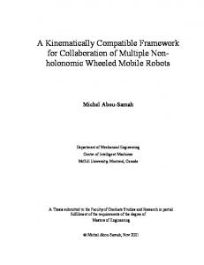
2 Discrete-time model The type of wheeled mobile robot considered in this work is shown in Figure 1. This class of robots, called twowheel differentially driven mobile robot consists of two parallel fixed wheels driven independently. A change of direction is obtained by the difference of velocity between the traction wheels. The continuous-time kinematic model of this mobile robot is well known in the literature [Campion et al., 96; Canudas et al., 96], and is given by
x&1 x& 2 θ&0
= u1 cosθ 0 = u1 sin θ 0 = u2 ,
(1)
where (x1 , x2 ) represents the coordinates of the center of the axle of the actuated wheels on the plane ( X 1 , X 2 ) and θ 0 is the angle that the longitudinal axis of the robot forms with the axis X 1 . The input signal u1 represents the
Computación y Sistemas Vol. 13 No. 2, 2009, pp 142-160 ISSN 1405-5546
144 Martin Velasco Villa, Eduardo Aranda Bricaire and Rodolfo Orosco Guerrero longitudinal velocity of the robot and u2 its angular velocity. In what follows, it is shown that an exact discrete-time model for system (1) can be obtained by direct integration. Consider a constant sampling period T and define the time interval between two consecutive sampling instants as, tk = {t ∈ R | kT ≤ t < (k + 1)T }, k = 0,1, 2,K
In the rest of the paper we assume that the control variables u1 (t ) and u2 (t ) remain constant between sampling instants (i.e. the inputs are sampled and connected to a zero order hold). Define u1 (kT ) and u 2 (kT ) as the constant values that the input signals u1 (t ) and u2 (t ) take over the time intervals tk for k = 0,1, 2, 3,K .
Fig. 1. Two-wheel differentially driven mobile robot
The equivalent discrete-time model for system (1) can be obtained by its direct integration over the interval tk . Considering first the evolution of θ 0 (t ) on equation (1), one readily obtains,
θ 0 (t ) = θ 0 (kT ) + (t − kT )u2 (kT ),
(2)
for t ∈ tk . Integrating now the first equation in (1) with θ 0 (t ) given as in (2) produces, x1 (t ) = x1 (kT ) + u1 (kT )
∫
t
kT
cos(θ 0 (kT ) + (τ − kT ) u 2 (kT ) ) dτ ,
that leads to,
x1 (t ) = x1 (kT ) +
u1 (kT ) [− sin θ 0 (kT ) + sin (θ 0 (kT ) + (t − kT ) u2 (kT ) )], u2 (kT )
Computación y Sistemas Vol. 13 No. 2, 2009, pp 142-160 ISSN 1405-5546
(3)
Discrete-Time Modeling and Path-Tracking for a Wheeled Mobile Robot
145
for t ∈ tk . Finally, from the second equation of (1) with θ 0 (t ) as in (2) we obtain x2 (t ) = x2 (kT ) + u1 (kT )
∫
t
kT
sin (θ 0 (kT ) + (τ − kT )u 2 (kT ) )dτ ,
that, evaluating the integral produces,
x2 (t ) = x2 (kT ) +
u1 (kT ) [cosθ 0 (kT ) − cos(θ 0 (kT ) + (t − kT )u2 (kT ) )], u2 (kT )
(4)
for t ∈ tk . In order to obtain the discrete-time model of the wheeled mobile robot (1), the equations (2), (3) and (4) are evaluated at the end of the interval tk , this is,
u1 (kT ) [− sin θ 0 (kT ) + sin (θ 0 (kT ) + Tu2 (kT ) )] u 2 (kT ) u (kT ) [cos θ 0 (kT ) − cos(θ 0 (kT ) + Tu 2 (kT ) )] x2 (kT + T ) = x2 (kT ) + 1 u 2 (kT ) θ 0 (kT + T ) = θ 0 (kT ) + Tu 2 (kT ). x1 (kT + T )
=
x1 (kT ) +
(5)
For the sake of simplicity, in the rest of the paper, the following notation is adopted ζ = ζ (kT ) ,
ζ = ζ (kT ± T ) and ζ [ ±i ] = ζ (kT ± iT ) . Using this notation and by means of simple algebraic manipulations, system ±
(5) can be rewritten as,
x1+ = x1 + 2u1ψ (u2 ) cos γ (θ 0 , u2 ) x2+ = x2 + 2u1ψ (u2 ) sin γ (θ 0 , u2 )
θ 0+
(6)
= θ 0 + u2T ,
Where
(
⎧ sin T2 u2 ⎪⎪ ψ (u2 ) = ⎨ u2 ⎪T ⎩⎪ 2
)
if u2 ≠ 0 if u2 = 0,
, γ (θ 0 , u2 ) = θ 0 +
T u2 . 2
Remark 2.1 Note that the function ψ satisfies, lim u2 →0 ψ (u 2 ) = T2 . In particular, when u2 = 0 the state θ 0 remains
constant accordingly to the property of the continuous-time model (1). It is easy to verify that the discrete-time model obtained from (1) when u2 = 0 corresponds to the discrete-time model (6) with ψ (0) = T2
3 Discrete-time control scheme In this section, the design of a commutation strategy for system (6) is developed. The control strategy achieves the path-tracking of a desired trajectory for the mobile robot based on the commutation between two discrete-time
Computación y Sistemas Vol. 13 No. 2, 2009, pp 142-160 ISSN 1405-5546
146 Martin Velasco Villa, Eduardo Aranda Bricaire and Rodolfo Orosco Guerrero nonlinear control laws. Both control laws linearize the input/output response of the system with respect to different output functions. The first output function possesses trivial zero dynamics. Therefore, the corresponding control law fully linearizes the system. The second output function exhibits zero dynamics of dimension one. The two output functions possess different singular manifolds. Therefore, a control switching strategy allows to construct a globally defined control law. In the continuous-time case, a nonlinear control via feedback linearization for the mobile robot (1) is commonly based on the output function h(x ) = [x1, x2 ]T . However, the consideration of this output function in the discrete-time case (6) does not produce the same result, it is a straightforward task to prove that, in this case, it is obtained an input-output linearization with unstable zero dynamics.
3.1 Dynamic extension
In order to obtain an equivalent control scheme that the one produced by considering h(x ) = [x1, x2 ]T in the continuous-time case, consider now, for the discrete-time counterpart, the output function, − − ⎡ h ( x,θ 0 ,θ 0− ) ⎤ ⎡ x sin θ 0 +θ 0 − x cos θ 0 +θ 0 ⎤ 1 2 2 2 ⎥. y=⎢ 1 = ⎢ ⎥ − ⎢⎣h2 ( x,θ 0 ,θ 0 )⎥⎦ ⎢⎣ ⎥⎦ θ 0−
(7)
Notice that this output function depends on the current and past values of θ 0 . In order to construct an output function defined only in terms of a classical realization it is necessary to define θ 0− as a new state, this is done by means of the following dynamic extension,
ξ1+ = θ 0 .
(8)
Therefore, for the augmented system (6)-(8) the output (7) is rewritten as
⎡ h ( x,θ 0 , ξ1 ) ⎤ ⎡ x1 sin θ 0 2+ξ1 − x2 cos θ 0 2+ξ1 ⎤ y=⎢ 1 ⎥. ⎥=⎢ ξ1. ⎥⎦ ⎣h2 ( x,θ 0 , ξ1 )⎦ ⎢⎣
(9)
System (6)-(8) with output function (7) possess a singular decoupling matrix [Kotta, 95; Nijmeijer and Van der Schaft, 90]. Therefore, in order to linearize the input/output response, it is proposed the dynamic extension,
u2 u1
= ξ 2 , ξ 2+ = w2 , = w1 ,
(10)
where w1 , w2 are new control inputs. This allows to rewrite (6)-(8)-(10) as the extended system,
x + = f (x, w), where, x = [x1, x2 , ξ1,θ 0 , ξ 2 ]T , w = [w1, w2 ]T and,
Computación y Sistemas Vol. 13 No. 2, 2009, pp 142-160 ISSN 1405-5546
(11)
Discrete-Time Modeling and Path-Tracking for a Wheeled Mobile Robot
147
⎡ x1 + 2ψ (ξ 2 ) w1 cos γ (θ 0 , ξ 2 )⎤ ⎢ ⎥ ⎢ x2 + 2ψ (ξ 2 ) w1 sin γ (θ 0 , ξ 2 )⎥ sin (T2 ξ 2 ) T ⎥ , ψ (ξ 2 ) = f ( x, w ) = ⎢ , γ (θ 0 , ξ 2 ) = θ 0 + ξ 2 . θ0 ξ2 2 ⎢ ⎥ θ 0 + Tξ 2 ⎢ ⎥ ⎢ ⎥ w2 ⎦ ⎣ Remark 3.1 The dynamic extension (8)-(10) depicted in Figure 2 amounts to add one pure time delay in front of the input u2 , and to store the value at the previous time instant of the variable θ 0 , in order to synthesize the linearizing control law.
Fig.2. Extended System (11) 3.2 Design of full linearizing control law In order to solve the path tracking problem, consider now the augmented system (11) and the output function (9). It is possible to compute for the component h1 ,
y1 = h1 (x ) = x1 sin
( )− x cos( ) θ 0 +ξ1 2
θ 0 +ξ1
2
2
( ) = x1 sin γ − x2 cos γ (x, w) = x1 sin γ + − x2 cos γ + − 2ψ (ξ 2 ) w1 sin (γ − γ + )
y1+ = h1+ x y1[ 2] = h1[ 2]
where γ + = θ 0 + Tξ 2 + T2 w2 . For the output component h2 , the first three forward shifts are given by
y 2 = h2 (x ) = ξ1
y 2+ = h2+ (x ) = θ 0
y 2[ 2] = h2[ 2] (x ) = θ 0 + Tξ 2
y 2[3] = h2[3] (x, w) = θ 0 + Tξ 2 + Tw2 .
Considering the functions y1[ 2] (x, w) , y2[3] (x, w) it is possible to write,
(
⎡ y1[ 2] ⎤ ⎡h1[ 2] ⎤ ⎡ x1 sin γ + − x2 cos γ + ⎤ ⎡− 2ψ (ξ 2 ) sin γ − γ + ⎢ [ 3] ⎥ = ⎢ [ 3] ⎥ = ⎢ ⎥+⎢ θ 0 + Tξ 2 0 ⎢⎣ h2 ⎦⎥ ⎣⎢ ⎦⎥ ⎣⎢ ⎣⎢ y2 ⎦⎥
)
0 ⎤ ⎡ w1 ⎤ ⎥ ⎢ ⎥. T ⎦⎥ ⎣ w2 ⎦
Computación y Sistemas Vol. 13 No. 2, 2009, pp 142-160 ISSN 1405-5546
148 Martin Velasco Villa, Eduardo Aranda Bricaire and Rodolfo Orosco Guerrero From the last equations, it is clear that the decoupling matrix ⎡− 2ψ (ξ 2 ) sin γ − γ + D=⎢ 0 ⎣⎢
(
)
0⎤ ⎥, T ⎦⎥
becomes singular on the manifold
2nπ 2mπ ⎫ ⎧ S = ⎨(x, ξ ) ∈ R5 | ξ 2 + w2 = ± or ξ 2 = ± , n = 0,1, 2..., m = 1, 2.....⎬ . T T ⎭ ⎩
(12)
Finally a feedback control law that solves the path tracking problem is given by 1 ⎤ ⎡ ( x1 sin φ − x2 cos φ − v1 )⎥ θ 0 − v2 ⎢ w ⎡ 1⎤ 2 sin ψ 2 ⎥, ⎢w ⎥ = ⎢ 1 ⎥ ⎣ 2⎦ ⎢ ( v 2 − θ 0 − Tξ 2 ) ⎥⎦ ⎢⎣ T
( )
where φ =
v2 +θ 0 +Tξ 2 2
(13)
and the new input variables v1 and v2 are,
v1 v2
= =
y1[d2 ] − k1e1+ − k0 e1 y2[ 3d] − m2 e2[ 2 ] − m1e2+ − m0 e2
(14)
with the output error ei = yi − yid . For the sake of conciseness, in the rest of the paper the control law (13)-(14) designed for system (11), will be referred to as w . For the closed loop system (11)-(13)-(14), the tracking error dynamics is governed by the difference equations
e1[ 2 ] + k1e1+ + k0 e1 e2[3] + m2 e2[ 2 ] + m1e2+ + m0 e2
= 0 = 0.
(15)
Remark 3.2 The relative degrees of system (11)-(9) are r1 = 2 , r2 = 3 and their sum is equal to the dimension of the extended system (11), then feedback law (13) fully linearizes the system. Remark 3.3 The control law w is undefined on the singular manifold S given in (12). 3.3 Complementary feedback law Since w is not defined on S , in order to obtain a global control scheme, an alternative control law with a different singular manifold is proposed. This alternative control law can be enabled when the state is in a neighborhood of S . To obtain this second feedback consider now the output function,
( )
⎡ h~ ( x,θ 0 , ξ1 ) ⎤ ⎡ x1 cos θ 0 +ξ1 + x2 sin ~ 2 y = ⎢ ~1 ⎥=⎢ h x θ ξ ( , , ) ξ1 ⎢ 0 1 ⎦ ⎣ ⎣ 2
Computación y Sistemas Vol. 13 No. 2, 2009, pp 142-160 ISSN 1405-5546
( )⎤⎥. θ 0 +ξ1 2
⎦⎥
(16)
Discrete-Time Modeling and Path-Tracking for a Wheeled Mobile Robot
149
Applying the same procedure as in the previous section it is obtained,
~ ⎡~ y1+ ⎤ ⎡ h1+ ⎤ ⎡ x1 cos γ + x2 sin γ ⎤ ⎡2ψ = ⎢ ~[3] ⎥ ⎢ ~[3] ⎥ = ⎢ ⎥+⎢ θ 0 + Tξ 2 ⎦ ⎣0 ⎣⎢ y2 ⎦⎥ ⎣⎢h2 ⎦⎥ ⎣
0 ⎤ ⎡ w1 ⎤ ⎢ ⎥. T ⎥⎦ ⎣ w2 ⎦
In this case, the decoupling matrix ~ = ⎡2ψ (ξ 2 ) 0 ⎤ D ⎢ 0 T ⎥⎦ ⎣
becomes singular on the manifold
2mπ ⎫ ~ ⎧ , m = 1, 2,K⎬. S = ⎨(x, ξ ) ∈ R5 | ξ 2 = ± T ⎩ ⎭
(17)
~ When the state does not belong to the manifold S , it is possible to synthesize the feedback law, ⎡ 1 ~ ⎤ (v − x cos γ − x2 sin γ )⎥ ⎡ w1 ⎤ ⎢ 2ψ 1 1 ⎥ ⎢w ⎥ = ⎢ 1 ~ ⎣ 2⎦ ⎢ ⎥ (v2 − θ 0 − Tξ 2 ) ⎢⎣ ⎥⎦ T
(18)
where v~1 and v~2 are given as,
v~1 v~2 with the output error
= =
~ ~ y1+d − k0 e~1 + ~ ~ e~[ 2 ] − m ~~ ~~ y2[ 3d] − m 2 2 1e2 − m0 e2 .
(19)
e~i = ~ yi − ~ yid .
~ . In Again, for sake of conciseness the control law (18)-(19) designed for system (11) will be referred to as w this case, the closed loop system (11)-(18)-(19) produces the tracking error dynamics
~ e~1+ + k0 ~ e1 [ 3 ] [ 2 ] + ~~ ~~ ~~ e~2 + m 2 e2 + m1e2 + m0 e2
=
0
= 0.
(20)
Remark 3.4 The relative degrees of system (11)-(16) are ~ r1 = 1 , ~ r2 = 3 and their sum is equal to four, therefore the extended system (11) under the control law (18) possesses a zero dynamics of dimension one.
~ is not defined when the state belongs to the singular manifold S~ given in (17). Remark 3.5 The control law w 3.4 Commutation strategy ~ The control scheme proposed in this subsection is based on the commutation between control laws w and w defined by (13)-(14) and (18)-(19), respectively. The singularities on the feedback (18) appear when the angular
Computación y Sistemas Vol. 13 No. 2, 2009, pp 142-160 ISSN 1405-5546
150 Martin Velasco Villa, Eduardo Aranda Bricaire and Rodolfo Orosco Guerrero velocity of the robot ξ 2 is equal to a multiple of the sampling frequency (17), i.e., ξ 2 = ± 2mT π . For most sampling periods considered for practical discrete-time applications ( T