take into account wheel slip give poor tracking performance for the WMR and path ..... time. The wheel torques, r, are related to the Cartesian force, E, and.
I26
lEEE TRANSACTIONS ON ROBOTICS AND AUTOMATION, VOL. I I , NO. I , FEBRUARY 1995
Modeling of Slip for Wheeled Mobile Robots R. Balakrishna and Ashitava Ghosal
Abstruct- Wheeled Mobile Robots (WMRs) are known to be nonholonomic systems, and most dynamic models of WMRs assume that the wheels undergo rolling without slipping. This paper deals with the problem of modeling and simulation of motion of a WMR when the conditions for rolling are not satisfied at the wheels. We use a traction model where the adhesion coefficient between the wheels of a WMR and a hard flat surface is a function of the wheel slip. This traction model is used in conjunction with the dynamic equations of motion to simulate the motion of the WMR. The simulations show that controllers which do not take into account wheel slip give poor tracking performance for the WMR and path deviation is small only for large adhesion coefficients. This work shows the importance of wheel slip and suggests use of accurate traction models for improving tracking performance of a WMR. Index Terms- Wheeled Mobile Robots, Slip, Modeling, Traction, Adhesion.
I. INTRODUCTION Wheeled Mobile Robots (WMRs) are generally modeled as nonholonomic dynamical systems with its wheels assumed to be rolling without slipping. The formulation based on rolling without slip gives kinematical mappings between wheel rotation and the position and orientation of the WMR. However, rolling conditions are sometimes violated in tractive maneuvering of WMRs, predominantly due to slipping and scrubbing [3]. In this paper, we use a model for the tractive force in terms of the adhesion coefficient, the linear and angular velocity of the wheel. The dynamic equations of motion are then derived including the effect of the tractive forces. It is shown that the equations of motion reduce to that obtained for 'ideal' rolling when no slip conditions are used. The 'ideal' rolling model is used to develop a model based controller. Simulation results with a PID controller and the model based controller show that the unmodeled slipping results in significant path deviation for the WMR, especially when adhesion coefficients are small. Hence, to obtain realistic models for maneuvering of WMRs, the rigid body dynamics of the WMR needs to be used in conjunction with slipping and tractive forces at the wheel-surface contact. Previous work in wheeled mobile robot modeling have neglected the aspect of wheel slip [I], [2], [19]. Other studies examined WMR maneuvering by considering the case when the torque applied does not exceed the traction limit [14]. The work presented by Alexander and Maddocks [3] predicts the resulting motion of a WMR by minimizing a friction functional when scrubbing takes place. Muir and Neuman [ l l ] , [12] describe methods to detect wheel slip and describe corrective measures. The modeling of tractive forces developed at the wheel has been used for various studies [18], [4], [8]. The model presented here has been widely used for automobile dynamic stability analysis [8], [17] and for traction control [16]. We discuss the model for wheel slip in Section 2. Manuscript received April 13, 1993; revised November 24, 1993. The author is with the Department of Mechanical Engineering, Indian Institute of Science, Bangalore 560 012 India. IEEE Log Number 94046 17.
The mechanical configuration of WMRs falls into one of two categories - steered-wheeled vehicles and differential-drive vehicles. This paper uses the latter category for simulation studies [9]. This paper is organized as follows: Section 2 presents the notion of wheel slip and wheel dynamics, Section 3 presents the Adhesion Coefficient model, Section 4 presents the WMR dynamic model with the wheel slip incorporated and control of the WMR is considered in Section 5. In Section 6 simulations for a 3 wheeled omni-wheeled mobile robot is discussed and in Section 7 we present our conclusions. 11. WHEEL- SLIP AND SINGLE WHEEL DYNAMICS
For a conventional wheel, the linear velocity of the wheel center, and wheel angular velocity, d, are related through the expression, 1' = r J,where r is the wheel radius. This expression represents 'ideal' rolling. This relation is a nonholonomic constraint between the variables 1 , and J. When the wheel rolls with slip this constraint is violated. To determine wheel slip between the wheel and a hard surface, it is assumed that the surface does not deform during traction but the wheel may undergo deformation at the contact patch. The wheel slip, A, can be defined as 11,
X =(H
- d * )/I)
(1)
where, d * is defined as P / I . with units of radsec, and is the wheel angular velocity in,radsec. The value of !/ is d' when J* > H and is i when J* < H . It may be observed that -1 5 X 5 1. For 'ideal' rolling, when d * = i , the wheel slip X is zero. When the linear velocity is zero, X = 1, and this represents the condition of wheel angular acceleration and rolling in place. The skid condition is characterized by zero angular velocity while the vehicle possesses a linear velocity. In this case X = -1. To represent the combined effects of rolling and slipping, the tractive forces of the wheel have to be introduced. The translational and rotational dynamics of a wheel of radius r , mass -\Itc,, and moment of inertia about the wheel center .Itc,,can be written as
where, Ft, is the tractive force developed at the wheel contact, .i: and H are the linear and angular acceleration of the wheel center, respectively, and T is the torque applied at the wheel axle. The above equations of motion for a single wheel undergoing rolVslip motion may be expressed in the state space form. Using the state vector, x = { . I , I . . 1 ' 2 . .r 1 . .I' I } , to represent the Cartesian position, linear velocity, angular rotation and angular velocity, respectively, we can write (2) as
'
or compactly as,
1O42-296x/95$04.O0 0 1995 IEEE
(3)
IEEE TRANSACTIONS ON ROBOTICS AND
AUTOMATION. VOL.
I I , NO. I , FEBRUARY 199.5
It can be observed that the translational and rotational dynamics for a wheel undergoing rolVslip motion are coupled through the tractive force Ft. It should be noted that the torque, T , is the only external independent input to this dynamical system. For this system to be locally controllable (see Isidori [lo], Spong and Vidyasagar [15]), the following vectors {g. u d ~ ( g ) .n d $ . (-y ) . , t d ' ; , ( ( / ) } should be linearly independent.' One can show that t r d : (g)becomes a zero vector if Ft is constant. Hence for the vectors t o be linearly independent, the tractive force Ft should be at least a C ' continuous function in .I'.L and . V I , which are the linear and angular velocities of the wheel. In the next section a traction model including the effects of wheel roll/slip will be described.
c
c
.-0,
~
-1.00
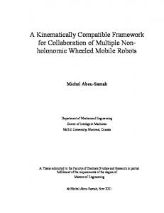
111. ADHESION COEFFICIENT MODEL The adhesion coefficient [I61 has also been referred to as the "friction coefficient" for wheel rolling [SI,and generally used as a measure to determine the adhesivity or sticking between two surfaces. The tractive force, F t , is generally obtained by the product of the adhesion coefficient and normal force at the point of contact. The adhesion coefficient is a function of the wheel dynamics and tractive conditions. It depends on quantities such as linear velocity of the wheel, the angular velocity of the wheel and the surface roughness in qualitative and quantitative aspects. Various models have been proposed for the tractive force, F f , in literature [4], 1181, [8].Unruh [I81 uses a model where the adhesion coefficient is assumed to be constant while Allen and O'Massey [4] assume a model where the adhesion coefficient is a function of the linear velocity. These models are useful only when the wheel is locked and the vehicle is skidding. We have used the traction model as proposed by Dugoff et al. [8]. The models presented here are for longitudinal wheel traction force.
Fig. 1.
i t versus X curve.
I
-E
E
I
I
Adhesion CoefJicient Dependent on Wheel Slip
In the model proposed by Dugoff et al. 181, the tractive force, F t , is a function of wheel slip, A(see Section 2). The tractive force, F t , is given by /trfAY, where p , is the adhesion coefficient and S is the normal reaction. 11. depends on the wheel slip, A, which in tum is a function of linear and angular velocities of the wheel. The tractive force developed is then formulated as
Ft = I / ( A ) S
(4)
The relation between the adhesion coefficient, p n , and wheel slip, A, depends on the nature of the surface and the wheel material [8]. A typical relationship is shown in Fig. 1 which shows the change in adhesion coefficient, p ", for acceleration and braking conditions. This curve has been proposed and verified by Dugoff et al. [8]. For a given surface and wheel material, it has been observed that though the quantitative characteristic of the curve may change, it matches qualitatively for different surfaces. Of particular significance is the peak value p n p p O k(shown in Fig. I), which is present for the acceleration and braking regions, with A taking positive and negative values, respectively. The adhesion coefficient, p r , , shows a rise and then a fall with increasing wheel-slip, A, where 0 5 1x1 5 1. The stable region is represented by the portion of the curve that shows an increase in the / t n with increase in A . In this portion, the tractive forces that can be sustained increases with the wheel-slip due to the increase in p , . The fall of p , , beyond the peak p o p ( , , l .results in instability since the tractive force reduces with increasing slip [16]. ' t r t l , (!/) -
tti/:.(y) ~
denotes the Lie Bracket of the two vector fields f &
= [. f . r , t l ~ - I- ( ( / ) ] and -
iid';.($
-
=0.
tj -
with
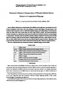
Fig.2. An Omni-wheel. It was observed in Section 2, that the controllability of a wheel is ensured if the tractive force model, F f ,is at least C 1 continuous in .1'2 and .I' I . The present adhesion coefficient model based on wheel-slip satisfies this criterion and also enables the representation of combined rolling and slipping in the wheel. In view of the above mentioned factors this adhesion coefficient model was used in the simulations. The lateral tractive force model for the wheel is not considered here, because the WMR considered in this work is a differential drive vehicle with omni-wheels. However, lateral tractive force can also be considered along similar lines [8], [17]. IV. WMR DYNAMIC MODELWITH WHEELSLIP The omni-wheel has freely rotating barrels at the periphery and the axis of rotation of the barrels are at an angle to the axis of rotation of the wheel. Thus, they have two degrees of freedom as opposed to conventional wheels which have one degree of freedom [I], 11 11. We consider a planar WMR with three omni-wheels and with barrels inclined at 90" to the wheel axis [9]. To ensure that the wheel always has two degrees of freedom, we consider a wheel having two layers of barrels as shown in Fig. 2. The kinematic and dynamics of WMRs (assuming no slip) with more than three wheels and with barrels inclined at other angles can also be derived [I], [2]. For the planar WMR with three omni-wheels placed at an angular separation of 120", shown in Fig. 3, one can find the relationship between the wheel variables and the Cartesian variables by using the no slip condition at the three wheels. Let the wheel rotational the wheel sliding speeds, speeds, { H I . H?. 4.1 }, be denoted by
i,
I zn
IEEE TRANSACTIONS ON ROBOTICS AND AUTOMATION, VOL. I I , NO. I , FEBRUARY 1995
Let -U,, be the mass of the WMR, I,, be the moment of inertia of the WMR about 2 axis, I, the moment of inertia of each wheel about its axis, and t' the radius of each omni-wheel. The kinetic energy of the WMR is given by the wheel rotational energy, and the WMR translational and rotational energies. The kinetic energy contribution of the barrels on the omni-wheel are neglected. The Lagrangian for the WMR is given as
xG
Using the Lagrangian formulation, we can derive the equations of motion for WMR systems as
${%}-% =F,.
,j = 1 ..... G
x3
Fig. 3 . WMR with coordinate frames and forces { m l . (TZ. m ~ } be , denoted by E.Since the motion of the WMR is in a plane, the velocity of any point G' (origin of the body fixed frame { G ' } )on the WMR, with respect to a fixed coordinate system, can be described by two components, { 1.1 1 L }, and the angular velocity of the WMR can be described by a single component \E normal to the platform. It may be noted that {I I 2 }, as shown in Fig. 3, are along -Yc;f and I;;( axes, respectively. We denote {I -1. I >. g} by I ? . It can be shown [l], that f and the Cartesian variables, E, are related by
.
.
where, r is the omni-wheel radius and L,. i = 1.2.3 are the distances of the omni-wheel contact point from G'. The [ R ] matrix relates f and and is analogous to Jacobian matrix in manipulators. The relationship between the sliding velocity of the omni-wheels, CJ, and the Cartesian velocities has been presented by Agullo er al. [l]. When the platform is rolling without slipping it has 3 degrees of freedom. However, when the rolling constraint is not satisfied, the I-, @ } WMR system has six degrees of freedom described by { Q are not and {HI. Ha. H:T}.This is because the 0's and 1-1. I related through the kinematic relations for 'ideal' rolling shown in (5). Let C: be the center of mass of the WMR. The frame {G} is aligned to the frame { G' } and has coordinates ( P I . p.2 ) with respect to { G' } as shown in Fig. 3. The velocity of the center of mass, with respect to a fixed frame, can be written as
>.
= {I; -
% Pa. I,
+%
PI
}'I.
(6)
where, C,is the Lagrangian of the WMR given in (7), q t . i = 1..... G is the set { S.I-. \E. H I . $2. 0.r } of generalized coordinates, and ;F are the generalized forces. The generalized forces corresponding to 0 , . i = 1.2.3 are T, - F t L r , i = 1.2.3 (see (3)). To obtain the generalized forces we have to write the F t , . i = 1.2.3 acting at the for (X. I-. 9), wheels along the Cartesian degrees of freedom. This can be done by use of the matrix [ R 1'' [ 2 ] . Hence the six generalized forces can be written as
; F = { t . [ R ] ' ( F 1 , . F l , . F l , ) " . ~ I- F t , t . . T J - F ~ , ~r :. < - F f 3 t * } . (9) The dynamic equations of motion for the WMR, including the effects of wheel slip, can be written as shown at the bottom of this page or compactly,
It may be noted that to arrive at the above equations, we have taken { G} and { G' } to be coinciding, i.e., e l = P Z = 0, I -1 = P I , 1-2 = 62 and L I = L Z = L.3 = L . It may be noted that the term % [ I) ] 1 arises because I -1 and I are components along the moving -Y(;, and I;;! axes and not along axis of the fixed coordinate system. We can make the following observations from the dynamic equations of motion. The individual wheel dynamics are coupled with the WMR dynamics through the tractive forces. The ideal rolling condition is not used. The only input to this model of the WMR are the wheel torques, T , . i = 1.2.3. The above equations of motion can be reduced to the equations of motion derived using the no slip conditions. This is shown below.
I29
IEEE TRANSACTIONS ON ROBOTICS AND AUTOMATION, VOL. 1 1 , NO. I , FEBRUARY 1995
The wheel dynamics alone are given by ( 1 1). Multiplying (1 1) by
[ R ] , and substituting for r [ R ] &, from (IO), we get [ R I ' [I]B+[.\f]li+\ir[C)]1=[R]'1.
(12)
i,=
The no-slip condition is given as [ R ] 1.Since [ R ] is a constant matrix, we obtain, = [ R ] 1, and on substituting them in ( I 2) and rearranging, we recover the WMR ideal dynamic equations (see Agullo et al. [2]). [:\I*]
li + 6 [ C)
] 1= [ R ]
(13)
Error Dynamics
The error dynamics for the WMR undergoing rolling with slip under the above model based control law is now presented. By substituting the expression for 1,(16). in (IO) and ( 1 1) and rearranging, we get
E,
V. CONTROL OF THE WMR The control problem for the WMR may be defined as that of guiding the WMR through a desired Cartesian path with specified terminal points. In this section, the path tracking performance of the WMR under PID control and a model based control using Cartesian space feedback is discussed. The Cartesian space feedback may be obtained either through dead reckoning or referential methods [6]. The dead reckoning method uses on-board sensors to estimate the current position of the WMR. In the present case, we assume that there are on-board sensors such as wheel encoders and accelerometers. PID Control
This control scheme uses the Cartesian space errors to compute the wheel torques according to the following PID control law
F
-=
Zi,.
(Xd-X)+Ii,,
(Xd-X)+Ii,
where X denotes the vector (S, I-. 9)' and Xd is the desired Cartesian space path and ( ) denotes the derivative with respect to time. The wheel torques, r, are related to the Cartesian force, E, and are given as
r = [ R I ' - ' E.
(15)
The dynamic model of the WMR is not used in this control scheme. Model-Based Control
The model based control approach seeks to exploit the model of the system to be controlled to obtain enhanced performance. The fundamental idea in this approach is to use the model of the system to be controlled in the control law, such that the resulting error equation is decoupled and linear, and is tunable by PID parameters [7]. In this section, we investigate the use of the dynamic equations of motion derived using the condition of 'ideal' rolling, (13) in the modelbased control law. One possible rationale for using the 'ideal' rolling model is that it is very hard to model adhesion coefficient and other nonlinearities of the real system. Assuming the availability of Cartesian space feedback and the reduced order 'ideal' rolling model, a model-based control law can be written as T = n i
+
,I
where, (1
=[ R
,I = [ R T' =
I-' 1- ' { \ir [ C) ] 1 }
X , / + Ii,( X