1 A bit on sampling distributions erm: sampdis.tex (draft) Nov 6, 2010. Note that a
sample mean, X, is a random variable # it varies from sample to sample.
1
A bit on sampling distributions
erm: sampdis.tex (draft) Nov 6, 2010 Note that a sample mean, X, is a random variable - it varies from sample to sample. Consider a sample of size n, (X1 ; X2 ; :::; Xn ). Then consider a function of of the sample f (X1 ; X2 ; :::; Xn ). Such a function is called a statistic, so we might want to write it s(X1 ; X2 ; :::; Xn ) X = s(X1 ; X2 ; :::; Xn ) =
1 n
n X
Xi is one example
i=1
Other examples are :5X1 + :25X2 , min(X1 ; X2 ; :::; Xn ), and X3 . All of these will take di¤erent values depending on speci…c sample drawn they have sampling variability. Since statistics are random variables, they have density functions (in this case called sampling distributions because the realization of the statistic will vary across samples) Understanding sampling distributions is at the foundation of understanding econometrics. For example, estimators (no matter how good or bad) have sampling distributions. We typically choose one estimator over another on the basis of the properties of their sampling distributions. That is, we choose the one with the ”better” sampling distribution.
1
Consider a random variable X with density function f (x) and mean
x.
Denote the density function for the sampling distribution of X, fX (x). In comparison, denote the sampling distribution of X3 , fX3 (x3 ), where X3 is the third observation in the sample. Two questions arise, what is the distribution/density function of a statistic, and what are its moments. Think about the expected values (means) of these two sampling distributions/density functions The mean of fX (x), E[X], is
x,
and the mean of fX3 (x3 ), E[X3 ] is
x.
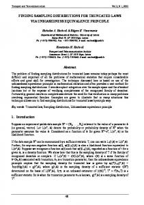
f(x b ar)1 .7 5 1 .5 1 .2 5 1 0 .7 5 0 .5 0 .2 5 0 0
0 .2 5
0 .5
0 .7 5
1 x b ar
Possible sampling distribution of X Does it surprise you that they have the same means. Another question is do X and X3 have the same density functions.
2
Consider var[X], when X is the mean of a random sample.
n
var[X]
= var[ =
=
1X Xi ] n i=1
n X 1 var[ Xi ] because var[aX] = a2 var[X] n2 i=1
1 var[X1 + X2 + ::: + Xn ] n2 1 (var[X1 ] + var[X2 ] + ::: + var[Xn ]) n2
because var[X1 + X2 ] = var[X1 ] + var[X2 ] if X1 and X2 are independent, which they are if it is a random sample. var[X] = That is var[X] =
2 x
n
1 (n n2
2 x)
=
2 x
n
. It decreases, approaching zero, as n approaches 1. 2
Summarizing E[X] = x and var[X] = nx 8 fX (x; the particular form of fX (x) if the sample is random.1
x;
2 x ),
independent of
1 Looking ahead, the sampling distribution of X approaches a normal distribution, independent of the distribution of X, as the sample size increases. This is the central limit theorem. That is, if the sample size is large enough, we know that X is approximately normally distributed with mean x and variance 2x =n.
3
What is var[X3 ] and how does it compare to var[X]? var[X3 ] =
2 x
2
Compare this with var[X] = nx . Both X and X3 are unbiased estimates of x but we prefer the former to the latter because it has a much smaller sampling variance. That is, we like its sampling distribution better because it is more concentrated around x . What to conclude? Ceteris, paribus, if two estimators are both unbiased. Go with the one that has the smaller sampling variance - one’s estimate is likely to be closer to the population parameter. If one wanted to estimate x with X, would you prefer a sample size of 2 1, n, or n + m? Why? Remember var[X] = nx . Ceteris paribus, more data/information is always better, assuming it is good data. Increasing the sample size, improves …nite-sample e¢ ciency, somthing we have not de…ned, yet.
4
1.1
Choose one or two other examples of statistics and derive the mean and variance of their sampling distributions.
For example, consider the statistic X=10. What is its expectation? What is its variance and how does it relate to the variance of X.
1.2
Deriving the sample distribution of a statistic, S
One way to derive/approximate the sampling distribution of a statistic is to simulate it. That is, draw a couple thousand random samples, calculate the statistic for each of the samples, and plot the distribution of the statistic across the samples. This is always possible, no matter how complicated the statistic. I want you to try this out in Mathematica. Specify a density function for a population. Don’t choose some standard run-of-the-mill distribution. Then choose a sampe size n, some speci…c number. Then specify some functional form for a statistic of this sample. Then choose some number of samples M . Draw M random samples, calculate the value of your statistic for each of your M samples, each of size n. Plot the sampling distributin of your statistic. Play around with di¤erent M , n and statistics. Maybe you could do this for a mixture distribution. That could be an assignment for one of the groups, Or, in contrast to stimulationg the sampling distribution, one can attempt to theoretically derive the sampling distribution of the statistic S = s(X1 ; X2 ; ::::; Xn ) based on fX (x) or FX (x), and the speci…cation of S = s(X1 ; X2 ; ::::; Xn ). The process by which this would be accomplished is not so di¢ cult to conceptualize, but often impossible to carry out in practice. More on this below. A lot of theoretical work in econometrics is derivations of sampling distributions of estimators.
1.2.1
The sampling distribution of X
Note that if, and only if, X~N ( x ; 2x ), is X~N ( For details see MGB (pp241 and 246)
5
x;
2 x =n)
However, there is a theorem called the Central Limit Theorem (MGB 234) that implies that if x1 ; x2 ; :::; xn is a random sample as n ! 1 fX (x) ! a normal distribution even if fX (x) is not Normal.2 This result will prove useful because often we cannot determine the form of fX (x) even though we know fX (x) often the Normal will be a fairly good approximation for fX (x), even when n is small. In theory, one could assume some arbitrary density function fX (x) and then theoretically derive the sampling distribution of X. However, this is often very di¢ cult, if not impossible. 2 Note that this theorem does not imply that for some other statistic, S, that as n ! 1 fS (s) ! a normal distribution
6
______________________________ 1.2.2
MGB (sec 3.2 ”Distribution on Minimum and Maximum) has some theorems on the distribution of max and min.
The following is an example of deriving the distribution of a statistic. Consider the rv Yn = max[X1 ; :::Xn ]. Yn which is a statistic. The probability that some number m is at least as large as the largest Xi in a sample of size n is Pr [X1 m; :::; Xn m] Said di¤erently, this is the probability that m is greater than or equal to all of the X 0 s in the sample. If the X’s are independent (for example, from a random sample) then Pr [X1 m; :::; Xn m] n n Y Y FXi (m) Pr[Xi m] = = i=1
i=1
So we have determined, in general terms, Pr [X1 m; :::; Xn m] if the X 0 s are from a random sample. But note that Pr [X1 m; :::; Xn m] = Pr[y < m] where y is the largest value of X. So,3 n Y Pr[y < m] = FYn (m) = FXi (m) i=1
And if X1 ; :::Xn , already assumed independently distributed, are also identically distributed with common cumulative distribution function FX (:), then Pr[y < m]
n
FYn (m) = [FX (m)]
We have just derived a sampling distribution for the statistic, the largest value of X in a sample of size n. A corollary: if X1 ; :::Xn are independent and identically distributed with common probability density function fX (:) and cumulative density function FX (:), then n 1 fYn (y) = n [FX (y)] fX (y) 3 Note that this formula works as long as the X are independent and allows for each of the i Xi to have a di¤erent CDF, so is not speci…c to random samples.
7
The corollary follows because it is always the case that
@F (x) @x
= f (x).
How does this apply to the sampling distribution of the max of a random sample from a univariate normal? The cdf for the max is the cdf for the normal raised to the power of the sample size.
8
1.2.3
More on deriving the sampling distribution of a statistic S = s(X1 ; X2 ; ::::; Xn )
As we did above, one can theoretically derive the sampling distribution of the statistic S = s(X1 ; X2 ; ::::; Xn ) based on fX (x) or FX (x), and the speci…cation of S = s(X1 ; X2 ; ::::; Xn ).
Before considering further the derivation of the distribution of a statistic, typically a function of a vector of random variables, consider deriving the the distribution of a single random variable, a simpler problem Derive fY (y) knowing y = g(x) and FX (x).
Consider …rst the derivation of the CDF of the sampling distribution of Y . We can often determine FY (m) from FX (x) by noting that FY (m) = Pr[y < m] = Pr[g(x) < m] because y = g(x)
In terms of the CDF FY (m) = FX (g(x) < m) = sistent with g(x) < m.
Z
fX (x)dx, the area under fX (x) con-
fx:g(x) g 1 (m)] = 1 FX (g 1 (m)) if
g(x) " x g(x) # x
Demonstrating with a the simpliest example, y1 = g1 (x) = x, where we know in advance that FY1 (m) = FX (m). Proceeding with the above steps, since g1 (x) is increasing in x FY1 (m) = Pr[g1 (x) < m] = Pr[x < g1 1 (m)] = Pr[x < m] = FX (m), which is correct. But now consider y2 = g2 (x) = x, where g2 (x) is decreasing in x. In this simple case, FY2 (m) = Pr[g2 (x) < m] = Pr[ x < m] = Pr[x > m] = 1 FX ( m), which is what one get if one applies the above equation for a decreasing function. That is, FY2 (m) = Pr[g2 (x) < m] = Pr[x > g2 1 (m)] = Pr[x > m] = 1 FX ( m) Demonstrating that the theorem is correct, at least, for g(x) = x and g(x) = x.
12
0
If, for example fX (x) = 1 if 0 x 1 and zero otherwise,
x
1 and zero otherwise() FX (x) = x if
8 < 0 if m if FY1 (m) = FX (m) = : 1 if
and
FY2 (m) = 1
FX ( m) =
Fy1 and Fy2
0
m1
8
0
1
0.75
0.5
0.25
0 -1.5
-1
-0.5
0
0.5
1
1.5 m
FY1 (m) in blue, FY2 (m) in red
13
Another example: if y = g(x) = ex , x = g FY (m) = So, if, for example, FX (x) = 1 m
1
0 if FX (ln m) if e
x
,x
6
(y) = ln y, m 0, strictly increasing in x. In which case
fY (m)
Alternatively, if fY (m)
dFX (x) dFX (g 1 (m)) d(g 1 (m)) = dx d(g 1 (m)) dm 1 d(g (m)) = fX (g 1 (m)) dm 1 d(g (m)) 7 = fX (g 1 (m)) dm =
dg(x) dx
0 (a restricted Beta distribution). In which case, fY (m)
= fX (g = a(e
1
m a 1
)
d(g
(m)) e
m
1
(m)) dm am
= ae
Graphing this for a = 2 fy and fx 2
1.5
1
0.5
0 0
0.5
1
1.5
2
2.5
3 m
fY (m) = 2e fY (m) = ae
am
2m
in red, fX (m) in blue
is the exponential distribution.
16
In turns out that we can often use fY (m) = fX (g g(x) is not strictly increasing or decreasing in x.
1
(m))
d(g
1 (m)) dm
even if
Consider a simple case where there are two segment: x < 0 and x 0 where dg(x) in one segment dg(x) dx > 0 and in the other dx < 0. Let gx