1 A Computational Intelligence Approach To Railway ...

1 A Computational Intelligence Approach To Railway Track Intervention Planning Derek Bartram1,3 , Michael Burrow2 , and Xin Yao3 1

2

3

Rail Research UK Gisbert Kapp Building The University of Birmingham Edgbaston, Birmingham B15 2TT, UK [email protected] Railways Group Department of Civil Engineering School of Engineering The University of Birmingham Edgbaston, Birmingham B15 2TT, UK [email protected] The Centre of Excellence for Research in Computational Intelligence and Applications (CERCIA) School of Computer Science The University of Birmingham Edgbaston, Birmingham B15 2TT, UK [email protected]

Summary. Railway track intervention planning is the process of specifying the location and time of required maintenance and renewal activities. To facilitate the process, decision support tools have been developed and typically use an expert system based approach with rules specified by track maintenance engineers. However, due to the complex interrelated nature of component deterioration it is problematic for an engineer, using a rule based approach, to consider all combinations of possible deterioration mechanisms. To address this, this chapter describes an approach to intervention planning which uses a variety of computational intelligence techniques. The proposed system learns rules for maintenance from historical data and incorporates future data as they become available thus improving the performance of the system over time. A failure type determination function analyses historical deterioration patterns of sections of track, and a Rival Penalized Competitive Learning algorithm determines possible failure types. A generalized two stage evolutionary algorithm is used to produce curve functions for this purpose. The approach is illustrated using an example with real data which demonstrates that the proposed methodology is suitable and effective for the task in hand.

2

Derek Bartram, Michael Burrow, and Xin Yao

1.1 Introduction There is a growing demand in many countries for railway travel, for example in the UK the demand for passenger transport has grown by over 40% in the past ten years [1]. As this demand is not being matched by the increased building of new railway track there is a constant pressure to improve reliability, efficiency and travel times of existing lines. This necessitates the use of faster vehicles with heavier axle loads and accelerates the rate of railway track deterioration. As the railway system deteriorates over time it is necessary periodically to maintain and renew components of the system. Such maintenance and renewal costs may be considerable for a large railway network and in the UK, for example, the annual cost of maintenance and renewal is approximately £4 billion [14]. In order to minimize expenditure on maintenance and renewal and at the same time maintain acceptable levels of safety, reliability and passenger comfort, it is necessary to have effective and reliable methods of predicting and planning railway track maintenance. These methods must analyze large amounts of data to enable current and future maintenance and renewal requirements to be determined. To facilitate this process a number of computer based systems have been developed for use in the railway industry as described below. The accuracy of these systems for maintenance and renewal planning however relies to a great extent on the availability of accurate, up to date, data and on expert judgment. This chapter describes an alternative approach based on a number of computational intelligence techniques, including evolutionary computation techniques, which are less reliant on the quality of the data and engineering judgment. In this chapter a new approach to railway track intervention planning systems is presented. In Section 1.2, Data for Prediction and Planning, and 1.3, Current Railway Track Procedures for Maintenance Management, available data generally available to the permanent way engineer is presented with a brief explanation of the methodology behind existing decision support systems and their inherent weaknesses. In Section 1.4, Our Proposed System, a new approach to decision support systems design is outlined along with the key issues facing the system and various ways how the issues may be overcome. Finally in Section 1.5, Prototype Implementation, an actual implementation of the proposed system is presented illustrating the various functions of the system.

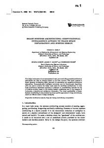
1.2 Data for Prediction and Planning Conventional railway track combines materials, such as the rail, rail pads, sleepers, ballast and sub-ballast, in a structural system (Figure 1.1). This system is designed to withstand the combined effects of traffic and climate to the extent that, for a predetermined period, the subgrade is adequately protected

1 Railway Track Intervention Planning

3

and that railway vehicle operating costs, safety and comfort of passenger are kept within acceptable limits [2]. As the system’s components deteriorate over time, measures of the condition of each of the components are collected to help make decisions regarding their maintenance and replacement (renewal). Typically data are collected on the mechanical condition of the ballast, fasteners and sleepers. Additionally data are collected on the number and types of rail failures (cracks and breaks), rail wear and rail corrugation (short wavelength defects which occur on the surface of the rail), and on the geometry of the track. The latter is the most widely used measure of the condition of the track for planning track maintenance and renewal and is described in more detail below. Structure.JPG

Fig. 1.1. Simplified Components of Conventional Ballasted Railway Track [2]

1.2.1 Geometry Measurements Railway track geometry Track data geometry collection A large amount of railway track maintenance expenditure results from adjusting the position and amount of the ballast under the track to correct the line and level. When the ballast can no longer be adjusted to maintain adequate geometry it is replaced (renewed). However, the process of determining the type, amount, location and timing of such maintenance or renewal activities is a complex task which requires track geometry deterioration to be predicted [7]. As sections of track may have dissimilar rates and mechanisms of deterioration, track geometry data are collected on short sections of track (typically less than 200 m). The principal measures of track geometry collected are changes in the vertical and horizontal geometry and the track gauge over time. Such measures are usually obtained by vehicles, known as track recording cars, details of which may be found elsewhere [7, 4].

4

Derek Bartram, Michael Burrow, and Xin Yao

1.2.2 Work History Data In addition to collecting data on the current condition of the track, historical data in terms of the type of maintenance and renewal work carried out at specific sites are usually recorded over a railway network. Such information may be used to help plan future maintenance and renewal activities. 1.2.3 Railway Standards A number of railways have issued standards related to the measures of track condition described above. These are used to help formulate rules regarding maintenance and renewal requirements (see below).

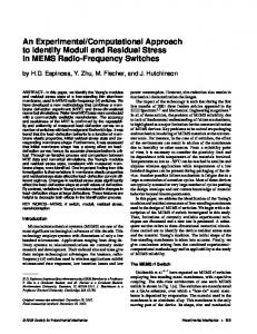
1.3 Current Railway Track Procedures for Maintenance Management Descision support systems Expert system As described above, managing track maintenance effectively and efficiently is a complex task. To address this, a number of computer-based systems have been developed to deal with the large amount of data collected. The majority of these are rule based systems and aim to produce information on the most appropriate type, location and time of maintenance and renewal of components through optimization processes. Rule based systems typically consist of four components, a knowledge base, a fact base, an inference engine and a diagnostic (see Figure 1.2).

Engine.jpg Fig. 1.2. Rule Based System Structure

In railway engineering, the knowledge base can be considered to contain information describing the type of components, physical location, age and associated measures of condition [21, 12]. In addition the knowledge base

1 Railway Track Intervention Planning

5

may contain information regarding the maximum permissible speed of each section of track, the annual tonnage of the trains using each section, as well as a record of historical maintenance. In some systems, information from the knowledge base is used to determine deterioration models for each component. These models estimate the rate at which a component may be expected to deteriorate and are used to help plan future maintenance based on the expected condition of a component. The fact base contains rules which are processed by the inference engine and used in combination with information in the knowledge base to form a diagnostic in terms of the type, timing and location of maintenance or renewal activities. Rules are typically of the form [15] IF (ConditionA ) . . . AND . . . (ConditionB ) . . . OR . . . (ConditionC ) THEN maintenance type and date For example [6], IF (Rail is of T ype A) AND (Speed ≤ 160km/h) AND (vertical wear of rail head in the track ≥ 8mm) THEN rail renewal required now While rule based systems are widely used, they have some inherent disadvantages, including; •

•

•

The quality of diagnostic is dependent upon the quality of the fact base and any errors or omissions in the fact base will result in the diagnostic being incorrect. The accuracy of the fact base are to a large extent based on the judgment of the engineers who have formulated them. Erroneous rules may result in a number of problems including maintenance and renewal work being scheduled early (and hence not being cost effective), scheduled late (and cause the track to fail comfort or safety specifications), or be of an incorrect type (which may result in only the symptoms of the underlying fault being treated). Furthermore, since the interrelation between the deterioration of all components in the track system is not fully understood, it is difficult for an engineer to define accurate rules which take into account these relationships. i.e. it is conceptually problematic to formulate rules which consider interactions between the rail, sleeper and ballast. As mentioned above, condition data are used to determine deterioration rates and models for components in isolation [6]. These models are often based on linear regression and represent a simplification of reality. Existing decision support systems are static solutions. Static solutions, once implemented, will always give the same result no matter how much data are processed by the system. Whilst static solutions may be dependable due to their predictability, as the quality of the system is dependent on the quality of the fact base, once an error is introduced into the system the error will always exist.

6

Derek Bartram, Michael Burrow, and Xin Yao

1.4 Our Proposed System 1.4.1 System Introduction System methodology This section describes a prototype system which uses computational intelligence and data mining techniques to produce a dynamically generated output. The system determines the diagnostics purely from historical data, and therefore overcomes the potential problems caused by domain expert knowledge (i.e. errors in the fact base). However, where there are insufficient historical data to enable an effective treatment to be suggested by the system, input from a permanent way engineer may be required. Using a system which derives its functionality from the data allows the system to be re-trained once more data have been acquired and hence, in theory, provide improved results each time new data are added. However, one problem using such a technique is that the initial resultant behaviour may be unpredictable. Furthermore, as the system considers all measures of track condition together, rather in isolation as is the case for the existing systems, it is able to take into account any interactions between the various track components. Consequently, the maintenance and renewal plans determined by our proposed system are likely to be more accurate than systems which are unable to consider component interaction. System Overview The proposed system performs two tasks; training and application. In the training stage, a number of processes are carried out as described below; 1. Various possible types of failures (including failures which behave differently according to usage, track design and subgrade conditions) are determined. It should be noted that these failure types may not be the same as those traditionally identified by an engineer since the system considers the interactions between components. 2. For the failure types identified above, deterioration models are produced for each of the recorded geometry measurements. 3. Determination of the various intervention levels. This process may be omitted as the values calculated should be the same as those given in the railway standards, however for ease of use and setup this process has been included. 4. For each failure type the most suitable type of maintenance or renewal is determined. 5. Training of a classification system to categorize new track sections into the previously discovered failure types. The system need only be trained once before use, however for the outputs of system to be improved over time, it should be periodically retrained as new data are added using the procedures described above. Retraining allows

1 Railway Track Intervention Planning

7

new failure types to be discovered and hence new deterioration models to be determined, thus improving the accuracy of the system outputs. Furthermore, as more data are added the deterioration models for all failure types can be regenerated increasing their accuracy. Once the system has been fully trained, the following results can be produced; 1. The current failure type(s) of the track 2. The optimal time to the next intervention. This is achieved by using each of the deterioration models for the determined failure type in conjunction with the standards to determine the geometry measurements that will exceed the standards 3. The most suitable intervention type for the determined failure type. 1.4.2 Missing and Erroneous Data Missing Data Eroneous Data In the railway industry during data capture it is possible to loose data for a number of reasons. These include; equipment error (incorrect setup or use) and measurement recorder out of bounds (particularly where the value measured is smaller / larger than the recorder can measure). Additionally, errors may be introduced in geometry recordings due to the limited accuracy of the recording tools used. Figures 1.3 and 1.4 show two different sections of track and the corresponding values of a measure of track quality, known as the standard deviation of vertical top height, (y axis) against time (x axis). As can be seen in both examples, no work history data are available (typically this would be shown as a vertical line separating two successive measurements). In such a case the data must be pre-processed as described below in order to make it suitable for further analysis. Figure 1.4 shows the extent of noise within the data, which appears to become ever larger in magnitude. From observation of a number of deterioration patterns it would appear that the noisy sections are periodic in nature. From the above it is evident that in order to produce a data driven approach to the problem described herein, three problems related to erroneous or missing data must be addressed as follows; • • •

Missing values Missing work history data Data noise.

These problems and their potential solutions are described below. Handling Missing Values Missing value substitution Removal of geometry measurements with a significantly high number of missing values removes any geometry measurement

8

Derek Bartram, Michael Burrow, and Xin Yao Deterioration Pattern.jpg Deterioration Pattern.jpg

Fig. 1.3. Real Data Run (1) Typical deterioration pattern Railway track deterioration

Fig. 1.4. Real Data Run (2)

where the percentage (or otherwise) of missing values for the measurement exceeds some critical value. This technique is very good for removing measurements specified as being recorded, but have not been in practice. However, when the number of missing measurements is significantly high in general (i.e. a high proportion of missing values across all geometry measurements), the technique performs poorly as too much data are discarded. Removal of geometry records with significantly high number of missing values discards records of geometry measurements with more than a critical number of missing values. This technique, like technique 1, has the disadvantage that a large amount of data are discarded from datasets with a significantly high number of missing values. Fill with a set value uses a predefined number inserted wherever a value is missing. This technique has the advantage of low complexity, however it will not perform well especially when an unsuitable value is chosen as the predefined number (e.g. a value outside the typical range for the measurement). Filling with a generated number is similar to filling with a set number but the number substituted is generated using an appropriate mathematical function, from the data itself. This technique has the advantage over substituting a predefined value as an appropriate function can be selected to generate missing values ensuring that the generated values are within the range of all possible values. In addition, it does not bias the data. However, when it is necessary to replace values in a time sequence of data, the technique can cause an atypical peak or trough to occur in the processed data when the missing value is not near the median. An example is shown in Figure 1.5 where the mean value is used to replace the missing data. However, as the missing value occurs very early on in the deterioration cycle the replaced value is inappropriately high and if used would suggest that the track condition has improved prior to any maintenance treatment. Replace missing values with a run generated value fits a curve (see Section 1.4.4 for curve fitting) to existing time series data to determine the missing value as shown

1 Railway Track Intervention Planning

9

in Figure 1.6 below. Even where the amount of data are limited it is still possible to produce a more appropriate substitution using this technique than using one of the four methods described above. From the expected nature of track deterioration observed in practice and described in the literature [21], a third order curve function may be suitable for this task (since it can capture both the post-intervention and pre-intervention increased deterioration rates). However, since data in any one particular run are often limited, for the more generalized case, a linear function may be used instead. While the example in Figure 1.6 shows excellent missing value substitution, it is worth noting that the accuracy of the technique is dependent on the order of curve chosen for the curve fitting routine. For example, if the missing value is at the end or beginning of a run and the curve shows a high degree of curvature due to an increasing deterioration rate pre and post intervention, using curve fitting of a higher order curve function is required. However, if too high an order curve function is used (i.e. overfitting) the value chosen for substitution may be outside the bounds of values found in practice (see Figure 1.7). Missing Value Via Averaging.JPG

Fig. 1.5. Missing Value Filling Via Generated Value

Handling Missing Work History Data In some datasets work history data may be missing and therefore prevents the generation of runs of data from sets of data. As a result it is not possible to determine deterioration models from the data. However, as the maintenance work may be expected to increase the quality of the track, track quality data should indicate an improvement when maintenance or renewal work has been carried out. Consequently, in many such cases it is possible to determine from the track quality data alone when maintenance or renewal work has been performed. This is demonstrated in Figure 1.8, where it may be seen that distinct improvements in track geometry quality have occurred (Figure 1.9). It is also interesting to note that in the example shown in Figure 1.9 using such information, it is possible to surmise further and determine whether the

10

Derek Bartram, Michael Burrow, and Xin Yao Missing Value Via Curve Fitting.JPG

Fig. 1.6. Missing Value Filling Via Run Curve Fitting Missing Value Via Poor Curve Fitting.JPG

Fig. 1.7. Missing Value Filled Via Poor Run Curve Fitting

intervention was maintenance or renewal work. Research suggests that after renewal the quality should be significantly better than after maintenance [21]. Accordingly with reference to Figure 1.9, the first and last interventions are likely to be renewals, while the middle two are more likely to be maintenance activities. Furthermore, the characteristics of a typical deterioration curve reported in the literature can also be seen from the figure. Just before and also after intervention the deterioration rate increases. Additionally, due to the effects of maintenance on the long term performance of the railway track after each maintenance activity the average deterioration rate over time increases. Handling Noisy Data Data noise Data scaling As shown in Figure 1.4, data may have a high degree of noise. To reduce its occurrence noise reduction techniques were used at two stages in the system training; once during the initial data processing stage (i.e. when the data runs are initially produced), and again later during the production of the deterioration models (during sampling for the genetic algorithms,

1 Railway Track Intervention Planning

11

With Work Data.JPG

Without Work Data.JPG

Fig. 1.8. Standard Deviation Of Vertical Top Height By Time, Without Work History Data

Fig. 1.9. Standard Deviation Of Vertical Top Height By Time, With Work History Data

see Section 2a, Deterioration Modelling). The noise reduction techniques use a similar curve fitting technique to that described above (see Section 1.4.2), and fit a third order curve to each run. During the process it is necessary to ensure that sufficient data are available within the geometry time series so that the curve is an accurate representation of the data. Once a curve function has been determined for a run of data, the real data are scaled to match the curve in one of three ways; complete (so that all geometry points lie on the curve function upon scaling), partial (so that all geometry points lie some percentage of the way towards the curve function), or graduated (where points with a higher deviation from the curve function are scaled more or less than those with less deviation). Figure 1.10 shows a set of data from two runs which has had the noise reduced (i.e. dark grey data to light grey data). In this example the data has been partially scaled to the curve function using a high scaling rate (i.e. a partial scaling with a relatively high percentage rate towards the curve function). Note however that the resultant data run does not necessarily show the expected trend of increasing in rate just prior and after intervention. The cause for this is currently unknown, but may be due to insufficient data to correctly train the curve fitting function. 1.4.3 Failure Types One of the main tasks in developing the proposed system is the determination of failure types. For the purposes of the proposed system, faults which deteriorate differently for different track components are considered to be separate failure types.

12

Derek Bartram, Michael Burrow, and Xin Yao With Work Data Denoised.JPG

Fig. 1.10. Real Data Before And After Noise Reduction

For the task two common clustering techniques, K Means [13] and RivalPenalized Clustering Learning (RPCL) [11], were considered and evaluated here for their effectiveness. For both techniques, a cluster centroid approach was adopted. In such an approach a point in n-dimension space represents the cluster and any geometry measurement (plotted within the same n-dimension space) is a member of the closest cluster centroid. Each cluster centroid therefore represents a single failure type. For the work described herein each geometry measurement is assigned to a single dimension of n-dimension space and the clustering algorithm clusters within that space. K Means Clustering K-Means is expressed in pseudo-code as follows [13]; • •

D is a dataset of i member elements d1 , d2 , d3 ...di C is the set of n cluster centroids c1 , c2 , c3 ...cn , where n is predefined by the implementation

foreach (cluster centroid c in C) { initialize c to a random position }

1 Railway Track Intervention Planning

13

do { foreach (dataset element d in D) { assign d to the nearest cluster centroid } foreach (cluster centroid c in C) { update c’s position to mean of all elements previously assigned to it unassign all elements from c } } until (all cluster centroids in C have not changed position since previous iteration) For the following sample dataset (Figure 1.11), the algorithm proceeds as follows; 1. From problem and domain knowledge, 2 clusters are known to exist, so 2 cluster centroids are initialized to random positions (Figure 1.12) 2. Data elements are assigned to the nearest cluster centroid (Figure 1.13) 3. Each cluster centroid is moved to the mean point of the average of all the points assigned to it (Figure 1.14) 4. Data elements are reassigned to the nearest cluster centre (Figure 1.15) 5. Cluster centroids are again moved to the centre of assigned data elements (Figure 1.16) 6. Data elements are reassigned to their nearest cluster centroid, however no elements are reassigned, and therefore clustering is complete. In the proposed system as mentioned above, it is not desirable for the railway engineer to have to specify the failure types nor their number, since it is possible that they may not identify certain failure types. Therefore in the proposed approach it is assumed that the number of clusters is not known and consequently it is probable that K Means will not perform well. Since the number of failure types is unknown an estimate must be used, however using an unrealistic estimate will cause problems. If the estimate is too high, then some clusters will be unnecessarily sub-divided (Figure 1.17), on the other hand an underestimate of the number of clusters can result in clusters being incorrectly joined(Figure 1.18). Rival Penalised Competitive Learning Rival-Penalized Clustering Learning (RPCL) is a modified version of the KMeans algorithm which uses a learning and de-learning rate to remove the need for prior knowledge of the number of clusters. However the learning and de-learning rates require careful tuning to the size and density of the required clusters [11]. In essence, RPCL performs similarly to K-Means with three modifications:

14

Derek Bartram, Michael Burrow, and Xin Yao Sample Data 7 k-means 1.jpg

Sample Data 7.jpg Fig. 1.11. Sample Clustering Dataset 1 Sample Data 7 k-means 2.jpg

Fig. 1.12. Dataset 1 With K Means Clustering (1) Sample Data 7 k-means 3.jpg

Fig. 1.13. Dataset 1 With K Means Clustering (2) Sample Data 7 k-means 4.jpg

Fig. 1.14. Dataset 1 With K Means Clustering (3) Sample Data 7 k-means 5.jpg

Fig. 1.15. Dataset 1 With K Means Clustering (4)

Fig. 1.16. Dataset 1 With K Means Clustering (5)

• •

•

Processing is performed on random data elements within the set, rather than all data elements nearest to the cluster centroid. Rather than moving cluster centroids to the mean position of assigned nodes, the closest cluster centroid is moved toward the randomly chosen point using a user specified learning rate. Unlike K-Means, RPCL moves the second closest cluster centroid (the rival) away from the randomly chosen point using a user specified delearning rate. RPCL is expressed in pseudo-code [11] as follows;

•

D is a dataset of i member elements d1 , d2 , d3 ...di

1 Railway Track Intervention Planning

15

Sample Data 1 clustered 2.jpg

Sample Data 1 clustered 3.jpg

Fig. 1.17. Over Estimate of Number of Clusters in K Means Clustering

Fig. 1.18. Under Estimate of Number Of Clusters in K Means Clustering

• • • •

C is the set of n cluster centroids c1 , c2 , c3 ...cn , where n is set to a value guaranteed to be greater than the actual number of clusters Learning rate ll is predefined in the range 0 < ll < 1 De-learning rate ld is predefined in the range 0 < ld < 1, and typically ld < ll Stopping criteria can be defined to best suit domain, however typically is a predefined number of iterations, or reduction of learning and de-learning rates each iteration until the learning rate or de-learning rate reaches a minimum bound.

initialize cluster centroids to random positions while (stopping criteria not met) { pick random data element dr from D determine closest cluster centroid cc to dr determine second closest cluster centroid cr to dr cc .position = cc .position + ll (dr .position - cc .position) cr .position = cr .position - ld (dr .position - cr .position) } For the following sample dataset (Figure 1.19) the algorithm proceeds as follows; 1. The number of clusters is unknown, but 3 was considered to be sufficient for this work (Figure 1.20). The literature varies on the best way

16

Derek Bartram, Michael Burrow, and Xin Yao

of determining a sufficient number [3], some favour selecting a very high number of clusters, while other suggest incrementing the number of clusters through repeated runs of the clustering algorithm until the number of output clusters does not change. 2. A random data element is chosen, and the winner (the grey cluster centroid) is learned towards it, and the rival (the white cluster centroid) is de-learned away from it (Figure 1.21). 3. The learning and de-learning rates are decreased. A new random element of data is choosen and the winner (the grey cluster centroid) is learned toward the point, and the rival (the black cluster centroid) is de-learned away from the point (Figure 1.22). 4. After a number of iterations the grey cluster centroid will tend towards the centre of the cluster, and the white and black cluster centroids will move further and further away (indicating they are unneeded). Depending upon the finishing criteria, the algorithm may finish at this point or continue. Should the algorithm continue at this point grey continues towards the centre of the cluster and the white and black cluster centroids continue towards infinity. Sample Data 8 rpcl 1.jpg

Sample Data 8.jpg Fig. 1.19. Sample Clustering Dataset 2 Sample Data 8 rpcl 2.jpg

Fig. 1.20. Dataset 2 With RPCL (1) Sample Data 8 rpcl 3.jpg

Fig. 1.21. Dataset 2 With RPCL (2)

Fig. 1.22. Dataset 3 With RPCL (3)

RPCL however has a disadvantage, associated with the relative size of the clusters, which is of a particular concern when used in the railway intervention planning domain. In the examples given above, the clusters were all of the same size, however when the clusters are formed from geometry measurements representing failure types the clusters are unlikely to be of a similar

1 Railway Track Intervention Planning

17

size since some failures are more common than others. Using RPCL, points are selected at random, therefore the cluster centroids of the smaller clusters will be selected at random less often than the next nearest clusters which are likely to be significantly bigger. The smaller clusters will thus, on average, be learned away more than they will be learned towards the smaller cluster. In the proposed system the problem of setting the learning and de-learning rate was addressed by first using the algorithm on a training set of data with known numbers of failure types and members. The training set was generated specifically for this task using ranges derived from actual data. The RPCL algorithm was used with different values until a good match between known properties of the training set and RPCL output was found. 1.4.4 Deterioration Modelling Using Evolutionary Approaches Deterioration modelling Railway track deterioration Genetic algorithm Evolutionary algorithm Curve fitting For each geometry measurement of each failure type, a deterioration model must be produced. Unlike existing decision support systems which use a fixed mathematical function fitted to the available data for a particular data set, the proposed system uses a two step genetic algorithm to learn a curve function. A second genetic algorithm is subsequently used to fit the curve function to the data. Using a two stage genetic algorithm provides several benefits. The main benefit is that the algorithm is able to generate a function automatically that will be able to model a typical deterioration curve, as well as any unusual deterioration patterns not normally considered. Furthermore, the genetic algorithm can use any standard mathematical function in conjunction with the known time since the last intervention, component ages, and traffic load. Since the curve function is built dynamically, it is also necessary to use a dynamic curve fitting function (i.e. a curve fitting function that fits to any curve, rather than a specific subsection of curves). Deterioration Modelling - An Example 1. Generate initial curve functions. Generalized curve functions are produced using random (but valid) combinations of the standard mathematical functions (+, -, *, /, Sin, Cos, Tan, ^ (power), etc), input variables (calculated from the data; time since last intervention and time since last replacement for each of rail, ballast, and sleeper), and algebraic constants (defined as ’a’, ’b’, ’c’, etc). Constants are only defined in one place per formula; however two constants may obtain the same value. To improve the performance of the algorithm, the selection of the various formula components are skewed towards a third order polynomial since this is the likely function format. The following illustates this process for a fictional dataset where Gm = ballastthickness.

18

Derek Bartram, Michael Burrow, and Xin Yao Modelling Flowchart.JPG

Fig. 1.23. Deterioration Model Generation Flowchart

Gm =

ballast age + b2 a

Gm = ballast age2 + b + sin(c)

(1.1) (1.2)

2. Train curve functions of population to data Each formula within the current population is trained one at a time. To reduce complexity however, the sampling of the dataset may be pre-computed so that the sampling is only performed once per formula generation, rather than multiple times per generation. a) If the dataset for training is sufficiently large (e.g. over 10,000 geometry records), a random sampling (approximately 1,000) is taken to reduce training time while still producing a good match to the original data. For each geometry record all input variables are calculated (i.e. ballast age since last intervention, ballast life span, rail age, etc.). Table 1.1 shows example data used for deterioration modelling. b) An initial random generation of constant values are generated. Assuming Formula 1 is being trained, then the following constant values may be generated (Table 1.2).

1 Railway Track Intervention Planning

19

Table 1.1. Example Training Dataset For Deterioration Modelling Ballast Thickness Ballast Age (days) Ballast Life Span (days) Rail Age (days) Etc... 25 27 28 27 29 25

15 30 42 32 48 17

15 30 42 32 48 17

1042 1057 1069 1059 1075 1044

... ... ... ... ... ...

c) The generation is evaluated using the following metric.

foreach (data row in training set) { calculate the difference between the formula output and desired result (i.e. geometry measurement) } calculate average of all differences

Using this metric requires trying to minimize the function and results in the output shown in table 1.3. Table 1.2. Generation 0 Values For Constant Training

Table 1.3. Metric Results, Generation 0

a

b

a

b

Metric

1 2 2 1.5 2

6 3.7 1 8 3.2

1 2 2 1.5 2

6 3.7 1 8 3.2

39.83333 4.396667 10.5 57.61111 4.086667

d) Test end criterion; for this example, the end criterion is to complete 2 generations (i.e. generations 0 and 1), and therefore is not met. e) The next generation is formed using the current generation. The constants are converted to 32bit binary representations and joined. Subsequently, the next generation is formed via the standard techniques of crossover, mutation, and copying, with tournament selection. Once the next generation of 32bit binary representations are formed, the reverse process of concatenation is applied resulting in the outputs shown in table 1.4.

20

Derek Bartram, Michael Burrow, and Xin Yao

f) The generation is evaluated using the curve function evaluation metric as above, resulting in the output given in table 1.5. Table 1.4. Generation 1 Curve Fitting Constant Values

Table 1.5. Metric Results, Generation 1

a

b

a

b

Metric

2 1.9 1.9 2.15 2.15

3.15 3.15 3.35 3.4 3.3

2 1.9 1.9 2.15 2.15

3.15 3.15 3.35 3.4 3.3

4.1925 4.174956 4.100482 3.669922 3.893256

g) Test end criterion; in this test, two generations have been completed, and so the following formula is returned back to the primary genetic algorithm. ballast age + 3.42 (1.3) 2.15 3. Once all formulae in the generation are trained, the end criterion is tested. The end criterion for this example is the fitness as evaluated by the secondary genetic algorithm and is less than 3.5. In an actual implementation this may be changed to a more complex metric and may include components such as the minimum number of generations and the change in the best, or average generation fitnesses. Equation 1.1 returned a best fitness of 3.669922, while equation 1.2 returned a best fitness of 12.387221; therefore the end criteria is not met and so the primary algorithm continues. 4. The next generation of formulae is generated by the primary algorithm, using standard tournament selection and crossover, mutation, and copying. Equation 1.1 is mutated to equation 1.4, and equation 1.1 and equation 1.2 are crossed over to form equation 1.4. Gm =

ballast age +b a

(1.4)

ballast age2 + b2 a

(1.5)

Gm = Gm =

5. Generation 1 is trained to data using the process described in ’Train curve functions of population to data’ previously. Since generation 0 was shown in detail, generation 1 will not be shown. 6. Test the end criteria; in generation 1, equation 1.4 returns a best fitness of 2.341 and therefore the primary genetic algorithm returns.

1 Railway Track Intervention Planning

21

Deterioration Modelling — Optimisation The process of deterioration modelling using a two stage genetic algorithm is highly computationally complex, and as a result takes a long time to complete. Consequently, two solutions to reduce the training time required were used as described below. 1. A distributed system [5] was used to enable more computers to process the task. Each instance of the secondary algorithm was assigned to a task, and sent to a single PC on a grid of computers. Consequently, as many instances exist per generation of the primary genetic algorithm (one per population member), the computation time was significantly reduced. 2. From experimental results the following observation of the secondary genetic algorithm was made (Figure 1.24). Fitting Training Trend.JPG

Fig. 1.24. General Quality Metric Per Generation Trend

As can be seen from Figure 1.24, after the initially fast improvement of quality, the rate of improvement decreases dramatically. Using this knowledge it is possible to set the secondary genetic algorithm to a short number of generations and obtain an approximation of the obtainable metric value. Running the secondary algorithm for a shorter period of time reduces the overall time for computation significantly. However, to maintain the quality of the output before the primary genetic algorithm terminates, the final output must be retrained to the original metric using the secondary genetic algorithm. 1.4.5 Works Programming Works programming is the process of determining the type of intervention to perform given the type of failure. Traditionally, works programming is

22

Derek Bartram, Michael Burrow, and Xin Yao

performed by a railway track engineer, however given the complexity of the domain of railway track intervention planning (i.e. the various components, interactions, materials, etc.) it is very difficult to specify the optimum intervention type in all cases. For this reason, as described above, historical data are used by the proposed system to determine the most suitable type of intervention per failure type. Heuristic Approach Heuristic works determination Intervention planning Railway track intervention planning For each failure type an intervention type must be determined and in the system the chosen type of intervention is then recommended for all sections of track which fail with that failure type. An intervention type determination metric is applied to each failure type as follows; foreach (run of data) { score the effectiveness of the following intervention using a metric M } foreach (intervention type) { calculate the average of all data runs which have a following intervention of that type } Select the intervention type with the highest average metric score At face value, the algorithm appears simplistic yet effective, however the complexity lies within the production of a scoring metric (M), as an ineffective metric results in a poor choice of intervention type. A number of factors have been considered in the research reported herein. However, when considered in isolation, they were not found to be suitable and therefore some combination of factors had to be chosen as described below. •

•

Using the length of time to the next intervention work as the sole parameter is unsuitable since a metric based on this parameter would result in renewal being predominantly chosen. While renewal would result in the minimum amount of maintenance being performed over time it is not necessarily the most cost effective intervention. Using a metric solely based on the next failure type is also unsuitable. Intervention work which is applied to a section of track which does not cause the failure type to change from what it was before the intervention to that afterwards, may be regarded to remedy the symptoms rather than the underlying cause of failure (i.e. the intervention may be regarded as

1 Railway Track Intervention Planning

23

cosmetic). However, when track is deteriorating at an optimal rate (i.e. when there are no underlying faults, but rather the deterioration is a result of normal use alone) a metric based on the next failure type would tend to result in an intervention type being suggested that would cause the track to deteriorate in a non-optimal way (i.e. resulting in a failure being introduced to the track, or being unnecessarily treated). The proposed system should be able to identify troublesome areas of railway track to the engineer. To this end, a procedure is proposed that enables the system to identify any sections of track where the selected intervention type’s metric score is less than a defined threshold value. Further, using this process the system is able to give a list of the intervention types that have been applied in the past to any type of failure and determine their effectiveness at remedying the failures. Conceptually, the intervention type determination process produces a directed non-fully connected graph of failure types, intervention types, and quality of intervention. Figure 1.25 shows a much simplified example. Type Linking Example.JPG

Fig. 1.25. Failure Type Linking

In practice it is more likely that for any given failure type and intervention type there will be more than one post intervention failure type. In such cases, a probability of the intervention resulting in the post intervention failure type is also included with the metric. This is based on the number of runs match-

24

Derek Bartram, Michael Burrow, and Xin Yao

ing the pre and post failure types and the total number of runs with that intervention type for those failure types. Life Cycle Costs The process of intervention type determination can be extended to take into account total life cycle costing. Existing solutions allow some total life cycle costing, however only on a macro scale (e.g. the costs associated with delaying a maintenance treatment by 6 months). By modifying the selection of the best average metric score in the intervention type determination metric to choose the intervention type with highest score of a second metric, a more sophisticated result can be obtained that takes into account factors such as cost and resource allocation. The second metric should take into account additional parameters such as the cost of the intervention work, age of components (to allow for older track to be replaced rather than repaired), and any other factors which may form part of the decision process normally used by an engineer.

1.5 Prototype Implementation In order to test the design of the proposed system, a prototype was developed as a proof of concept. In this section, the significant parts of the prototype are described and discussed. 1.5.1 System Training Before any sections of track can be processed the system is initialised, This requires the user to carry out a number of processes, each of which are described in several dialog boxes (Figure 1.26). Since the engineer may not be fully conversant with the system, the dialog is designed to lead the engineer through the process of preparing the database for intervention planning; the following describes the function of each stage of this process. 1. Database connection; before any processing can be started, the location of the data is specified. Table 1.6 shows a partial knowledge base comprising geometry measurements taken over a section of line (AAV1100) from 29125km to 29625km, over a number of geometry recording runs (i.e. runs from 28/11/1997 to 17/02/2001). 2. Filtering for missing data: in the proposed system both geometry types and geometry records are removed if more than 60% of the geometry measurements or 60% of the geometry record is missing. During this phase a unique identifier (UID) is added to the geometry and work history values so that they can be referenced later. Since UID, Line Track ID, From, To, and Date are required they are not removed by filtering. However they are

29250 29250 29375 29375 29375 29375 29500 29500 29500 29500 29500 29625 29625 29625

02/08/2000 05/06/1998 17/02/2001 05/06/1998 02/08/2000 04/11/1998 17/02/2001 28/11/1997 04/11/1998 02/08/2000 05/06/1998 28/11/1997 17/02/2001 05/06/1998

29125 29125 29250 29250 29250 29250 29375 29375 29375 29375 29375 29500 29500 29500

AAV1100 AAV1100 AAV1100 AAV1100 AAV1100 AAV1100 AAV1100 AAV1100 AAV1100 AAV1100 AAV1100 AAV1100 AAV1100 AAV1100

02/08/2000 05/06/1998 17/02/2001 05/06/1998 02/08/2000 04/11/1998 17/02/2001 28/11/1997 04/11/1998 02/08/2000 05/06/1998 28/11/1997 17/02/2001 05/06/1998

Date

LineTrackID CampaignID From To True True True True True True True True True True True True True True

4.8 4.5 NULL 5.1 4.9 NULL NULL 2.4 NULL 2.5 2.4 NULL 3.5 NULL

0 0 NULL 0 0 NULL NULL 0 NULL 0 0 NULL 0 NULL

0 0 NULL 1 2 NULL NULL 0 NULL 0 0 NULL 0 NULL

NULL NULL NULL NULL NULL NULL NULL NULL NULL NULL NULL NULL NULL NULL

1445 1454 1445 1445 1441 1446 1441 1436 1439 1435 1440 NULL 1438 NULL

Flag Abs Alignment Abs Vertical Abs Twist Abs Crosslevel Abs Gauge

Table 1.6. Sample Geometry Data

1 Railway Track Intervention Planning 25

26

Derek Bartram, Michael Burrow, and Xin Yao Application V3.JPG

Fig. 1.26. System Preparation Dialog

marked as linking columns so that they are not processed. Flag is removed since all values for this measurement are the same and therefore it would not be able to distinguish anything using this measurement. Measures of track geometry as specified by, Abs Vertical and Abs Gauge are kept as less than 60% of their values are missing. However, the measures of track geometry specified by Abs Twist and Abs Crosslevel have over 60% of their values missing and are therefore discarded. 3. In order to produce sets of runs work data are merged together with the geometry data (i.e. a linked form using the unique identifiers previously added). 4. For each column of data null values are filled using the mean of values in the column. Whist this method has proved satisfactory so far, it is anticipated that further research will be performed to determine the effect of the various missing value substitution techniques described earlier (see Section 1.4.2). 5. Values are converted from absolute values to relative values in order to make a valid comparison between different track sections. A direct comparison is not possible as some geometry measurements may be different between track sections due to differences in track design. The process scales each run of data to an initial base value of 100, converting absolute values of geometry measurement to a percentage of the initial run measurement.

1 Railway Track Intervention Planning

27

6. Clustering is performed. During this phase, an RPCL algorithm is applied to the last geometry measurement of each geometry run to determine failure types. 7. Cluster filtering is performed to remove excess clusters which do not correspond to failure types. A cluster is removed if it contains less than a specified number of geometry measurements (e.g. 20). This process removes clusters tending away from the geometry measurements (see Section 1.4.3). 8. Cluster definitions, defining the regions covered by each cluster, are produced. 9. Intervention levels and initial geometry levels are determined. 10. Work types and costs are determined. 11. Failure type linking is performed, resulting in a failure type linking chart (see Section 1.4.5). 1.5.2 Intervention Planning Intervention planning can be performed once the system has been fully trained. Selection Creation Before an intervention plan can be produced, the track sections to be analyzed are specified via the ’New Selection’ dialog (Figure 1.27). The new selection dialog contains three parts; general settings allows naming and access rights to be set; the left hand tree list contains all possible track sections in which can be used to form a selection; the right hand list specifies the track sections which have been added to the selection and provides a means (via the use of buttons) of adding and removing track sections from the selection. In figure 27, a new selection named ’Selection 1’ been created; the selection contains line track ID 00133 from 73234km to 74634km. Line track ID 01301 has been selected to add to the selection. In addition the user has used a feature to highlight all references containing 013 (this feature allows the quick selection of multi track sections conforming to a specific rule; once highlighted the sections can be quickly and easily added to a selection). Finally the user has specified that the system should open the selection once finalized (see Section 1.5.2 below). Selection View The selection view (Figure 1.28) allows the user to display various pieces of information about the specified selection, including the most recent geometry measurements for each section of the selection. Geometry data can be viewed in a number of common formats and at various scales. In addition, historical

28

Derek Bartram, Michael Burrow, and Xin Yao Selection Dialog.JPG

Fig. 1.27. Create Selection Dialog

data can be viewed by moving the mouse over the relevant section of track and geometry measurement. The current and historical failure type classifications can be displayed in a similar manner and are colour coded to match the settings dialog. Intervention Plan The intervention plan view (Figure 1.29) is currently under development, and therefore only displays performed work history data, however in future versions of the prototype it is anticipated that it will also display recommended work. Each intervention is represented by a grey mark at the relevant section and date. Further information such as cost, location, and type can be displayed by moving the mouse over the corresponding intervention work item. Analysis Tools To aid in the development and testing of the prototype, several tools were created as follows; •

A statistical analysis tool was developed which allows the analysis of the raw data. This tool allows the percentage and frequency distribution of missing values to be determined. For the former both the percentage of missing values per column (e.g. track geometry value) and by row (i.e. by

1 Railway Track Intervention Planning

29

View.JPG

Fig. 1.28. Selection Data View

•

geometry record) can be determined. The frequency distribution of values specifies the top 15 most common values per column (as before). The statistical analysis tool can also be used to produce a raw view of each set of data (e.g. geometry and work history data as per figures 1.3 and 1.4). 1.7 shows a partial output for the statistic analysis tool. As can been seen, a high degree of missing values is present indicating that the dataset is of poor quality. The Primary Classification Evaluation Tool was designed to display the effectiveness of the primary classification system. This is achieved by parsing the training set used in generating the primary classification system back through the primary classifier to compare the output of the classifier with the known failure type. The geometry data points are coloured depending on the result of the comparison. Green is used to indicate a positive match (i.e. the classifier has determined the correct failure type), aqua to indicate that the classifier determined a number of failure types of which one was correct, orange that multiple incorrect classifications were determined, and red to indicate the classification system produced one failure type which was incorrect. It was expected that beyond the region of initially good track quality, the clusters diverge and can be differentiated via the primary classification system. In the example presented in Figure 1.30, the classification rate is poor across the whole range of geom-

30

Derek Bartram, Michael Burrow, and Xin Yao View.JPG

Fig. 1.29. Intervention Plan Dialog

•

etry values, indicating that the primary classification system is ineffective. For the older track geometry recordings (i.e. rightmost), the classification appears to be somewhat improved, however this is most likely to be due to overlapping clusters becoming increasingly large, until the largest just includes all of the data. Failure types can be analyzed via the Failure Type Linking Analysis Tool. The tool allows each failure type to be viewed and allows the effect of maintenance to be determined. In the example shown in Figure 1.31, a track section which deteriorates with Failure Type 1 has been treated with maintenance type T and then subsequently deteriorates with Failure Type 3. In some cases, as can be seen with Failure Type 3, given any type of maintenance, post intervention the track section will still deteriorate with Failure Type 3. Such a scenario may be due to either the maintenance types performed on this failure type in the past having only treated the symptoms (and hence the underlying cause remains), or the track is deteriorating in the optimal manner (i.e. there are no specific faults with the track section but rather it is failing due to general use). In Figure 1.31, the popup box shows information corresponding to the link between Failure Type 3 and Failure Type 2. In addition information relevant to the pre and post intervention is displayed, along with information relevant to the type of intervention. In cases where given a particular failure type and intervention type, there are multiple post intervention failure types, the probability of post intervention failure type is displayed on the link. The

1 Railway Track Intervention Planning

31

Table 1.7. Sample Statistical Data For Geometry Table Column Name

Average Number Of Number Of Missing Values Missing Value Percentage

LineTrackID CampaignID GeomFrom GeomTo GeomDate GeomFlag GeomAbsAlignment GeomAbsVertical GeomAbsTwist GeomAbsCrosslevel GeomAbsGauge GeomAbsValue GeomSDAlignment GeomSDVertical GeomSDTwist GeomSDCrosslevel GeomSDGauge GeomSDValue GeomFaultsAlignment GeomFaultsVertical GeomFaultsTwist GeomFaultsCrosslevel GeomFaultsGauge GeomFaultsValue GeomSecurityAlignment GeomSecurityVertical GeomSecurityTwist GeomSecurityCrosslevel GeomSecurityGauge GeomSecurityValue GeomQuality

NaN NaN 67064.53 67189.35 NaN NaN 2.80 0.00 0.10 0 1436.80 2.77 1.41 2.60 2.16 1.74 0 3.48 0.02 0.06 0.08 0.00 0.05 0 0.08 2.89 0.67 0.98 0.24 0 4.34

0 0 0 0 0 0 1270513 1272271 1272271 1394180 1282211 282606 91456 54429 48440 1272140 2091646 218747 1309606 1274511 1272828 1273976 1297574 1349403 1316366 1294169 1272828 1291836 1297474 1349403 30208

0 0 0 0 0 0 60 60 60 66 61 13 4 2 2 60 100 10 62 60 60 60 62 64 62 61 60 61 62 64 1

system displays the best probability / link in the given example for clarity of presentation.

1.6 Conclusions Existing decision support systems for railway track intervention planning is sub-optimal in dealing with the complexity of intervention planning. In particular, the fact base containing the rules in a typical expert system structure

32

Derek Bartram, Michael Burrow, and Xin Yao Classification Evaluation.JPG

Fig. 1.30. Primary Classification Evaluation Tool

of existing decision support tools may be regarded as having overly simplistic deterioration models which are unable to describe the complex interactions between track components. To address these issues a data driven computational intelligence approach to railway track intervention planning system was presented in this chapter. The proposed system uses a variety of computational intelligence techniques, including clustering to determine the various failure types applicable to track deterioration, evolutionary algorithms to produce deterioration models for each failure type, and a heuristic based approach to determine the most appropriate maintenance to perform per failure type. In the proposed system, a number of novel processes and techniques have been adopted, including the methodology of deriving the functionality of the system from the available data itself without the need for expert judgment. Furthermore, the proposed system can determine the possible types of failure by which a selected section of track can deteriorate (including the degree of track affected by such failure), and the interaction between intervention types and failure types. While the system may not be able to provide names for track failure types in terms readily recognised by a railway engineer, combined with the knowledge of the engineer, the system can produce a highly detailed history (or prediction) of the changing state of a given section of track. From a computer science aspect, the system also contains novel aspects, e.g., techniques used to determine failure types and the production of deteri-

1 Railway Track Intervention Planning

33

Type Linking.JPG

Fig. 1.31. Failure Type Linking Analysis Tool

oration models. In the determination of failure types, a clustering algorithm was used on railway track geometry data. To overcome the typically used trial and error approach to tune clustering algorithms a training set, with a known number of failure types and members, was produced which mimicked the behaviour of a simplistic real data set. The training set was processed using the clustering algorithm until the output from the clustering algorithm matched the known properties of the training set. The two stage evolutionary algorithm used for the production of deterioration models is also innovative as the second evolutionary algorithm was used in conjunction to train the generations of the first evolutionary algorithm. This system, once tuned, enables curve fitting (and optimization) to be performed on any set of data, and not just that of railway track geometry data. 1.6.1 Strengths of the Proposed System •

•

Improvement over time: The proposed system can be retrained as and when more data are available, thus improving the accuracy of the output. As more track condition data becomes available the system may find new undiscovered failure types. Furthermore, more data are available for the production of deterioration models, and also for use in the heuristic based approach to intervention type determination. The behaviour of the system is defined by historical data: The behaviour of existing systems is set by engineers, and therefore any mistakes or omissions added to the fact base results in a system that performs incorrectly,

34

•

Derek Bartram, Michael Burrow, and Xin Yao

or at best non-optimally. Using behaviour generated from historical data ensures that the system will perform at worst, as well as systems used in the past. Identification of weak areas of diagnostic: existing systems give only very general indications of the quality of intervention plans, whereas the proposed system is able to identify problem areas more specifically.

1.6.2 Weaknesses of the Proposed System The weaknesses of the proposed system are related to the reliance of the system on historical data; •

•

•

Since the proposed system is defined by historical data, a high quality dataset with few errors and missing values must be used to train the system. The historical data used for training the proposed system must already contain railway track which has been treated in a suitable manner, otherwise the system will not initially perform well. Furthermore, the quality of the intervention plans produced is dependant on the quality of the treatment within the historical data. While the system is able to identify poorly treated sections of track historically, it is not able to determine the effect of a treatment previously unused upon a particular failure type. The historical data must be representative of the types of track for which intervention plans are being generated. If a track section has a failure type previously unseen by the system, then the output of the system is undefined and unknown.

1.6.3 Areas for Further Research The following items of further research are recommended; • • •

Uncertainty of classification of sections with failure types unknown to the system (i.e. not in historical data) Varying section size Total life cycle costing; optimization; including coherence processing.

References 1. Association of Train Operating Companies (2005), Ten-Year European Rail Growth Trends, The Association of Train Operating Companies, London, UK., 1 July 2006 2. Burrow, M.P.N., Ghataora, G.S & Bowness, D., Analytical track substructure design. ISSMGE TC3 International Seminar on Geotechnics in Pavement and Railway Design and Construction, NTUA - Athens, 16-17 December 2004., pp. 209–216

1 Railway Track Intervention Planning

35

3. Cheung, Y., A Competitive and Cooperative Learning Approach to Robust Data Clustering, IASTED International Coference on Neural Networks and Computational Intelligence, 23-25 February 2004, pp. 131–136 4. Cope, G.H., British Railway Track — Design, Construction and Maintenance, The Permanent Way Institution, Eco Press. Loughborough, UK., 1993 5. Coulouris, G.F., Dollimore, J. & Kindberg, T., Distributed Systems: Concepts and Design, Third Edition. International Computer Science, 23 August 2000, pp. 28–64 6. ERRI, EcoTrack - Decision Support System for Permanent Way Maintenance and Renewal - Specifications 1. General Concept, ERRI, April 1994 7. Esveld, C., Modern Railway Track, Second Edition. MRT-Productions, Zaltbommel, The Netherlands., August 2001 8. Jovanovic, S., Optimal Resource Allocation Within the Field of Railway Track Maintenance and Renewal, Railway Engineering 2000, London, 5-6 July 2000 9. Jovanovic, S. & Esveld, C., An Objective Condition-based Decision Support System for Long-term Track Maintenance and Renewal Planning, 7th International Heavy Haul Conference, Australia, 10-14 June 2001, pp. 199–207 10. Jovanovic, S. & Zaalberg, H., EcoTrack - Two Years of Experience, Rail International, April 2000, pp. 2–8 11. King, I. & Lau, T., Non-Hierarchical Clustering with Rival Penalized Competitive Learning for Information Retrieval, First International Workshop on Machine Learning and Data Mining in Pattern Recognition, 16-18 September 1999, pp. 116-130 12. Leeuwen, R.V., The EcoTrack Project - Effective Management of Track Maintenance, Belgium National Railway Company, Brussels, 1996, pp. 1–16 13. Moore, A.W., K-means and Hierarchical Clustering, Carnegie Mellon University, 8 October 2004 14. Network Rail, Business Plan, Network Rail, UK., 4 April 2006 15. Stirling, A.B., Roberts, C.M., Chan, A.H.C., Madelin, K.B. & Bocking, A., Development of a Rule Base (Code of Practice) for the Maintenance of Plain Line Track in the UK to be used in an Expert System, Railway Engineering 1999, London, 26-27 May 1999 16. Stirling, A.B., Roberts, C.M., Chan, A.H.C., Madelin, K.B. & Vernon, K., Trial of an Expert System for the Maintenance of Plain Line Track in the UK, Railway Engineering 2000, London, 5-6 July 2000 17. Stirling, A.B., Roberts, C.M., Chan, A.H.C. & Madelin, K.B., Prototype Expert System for the Maintenance and Renewal of Railway Track, Freight Vehicle Design Workshop, Manchester, 2000 18. Rivier, R. & Korpanec, I., EcoTrack - A Tool to Reduce the Life Cycle Costs of the Track, World Congress on Railway Research, 16-19 November 1997, pp. 289–295 19. Rivier, R.E., EcoTrack - A Tool for Track Maintenance and Renewal Managers, Computational Mechanics Publications, Institute of Transportation and Planning, Swiss Federal, September 1998, pp. 733–742 20. Roberts, C., A Decision Support System for Effective Track Maintenance and Renewal, PhD Thesis, The University of Birmingham, January 2001, pp. 1–395 21. Roberts, C., Decision Support System for Track Renewal Strategies and Maintenance Optimization, Railway Engineering 2001, 30 April-1 May 2001 22. Zaa, P.H., Economizing Track Renewal and Maintenance with EcoTrack, Cost Effectiveness and Safety Aspects of Railway Track, Paris, 1998

36

Derek Bartram, Michael Burrow, and Xin Yao

Acknowledgements The financial support of the Engineering and Physical Sciences Research Council is noted with gratitude. The authors also wish to thank the practical and financial support of the Schools of Computer Science and Engineering at the University of Birmingham.