TRAC-IT is a mobile phone application that records travel behavior by collecting real-time GPS data and requiring minimal input from the user for data such as.
AUTOMATING MODE DETECTION USING NEURAL NETWORKS AND ASSISTED GPS DATA COLLECTED USING GPS-ENABLED MOBILE PHONES Paola A. Gonzalez, Jeremy S. Weinstein, Sean J. Barbeau, Miguel A. Labrador, Philip L. Winters, Nevine Labib Georggi, Rafael Perez Center for Urban Transportation Research and Department of Computer Science & Engineering University of South Florida Tampa, Florida 33620 (pagonzal, weinstein, barbeau, winters, georggi) @cutr.usf.edu (perez, labrador) @cse.usf.edu
ABSTRACT Next-generation transportation surveys will utilize Global Positioning Systems (GPS) to collect trip data. Due to their ubiquity, GPS-enabled mobile devices are becoming promising for use as survey tools. TRAC-IT is a mobile phone application that records travel behavior by collecting real-time GPS data and requiring minimal input from the user for data such as trip purpose, mode of transportation, and vehicle occupancy. To ease survey burden on participants, new techniques must be explored to derive more information directly from GPS data. This paper demonstrates the feasibility of using neural networks and assisted GPS data collected from GPS-enabled mobile phones to automatically detect the mode of transportation. Furthermore, this paper demonstrates that this technique can be optimized using a critical point algorithm to reduce the size of required GPS datasets obtained from GPS-enabled mobile phones, thus reducing data collection costs while saving mobile phone resources such as battery life. Keywords – location based services, GPS, mobile phones, cell phones, mode detection, neural network, travel behavior, GIS, TRAC-IT INTRODUCTION AND MOTIVATION Travel surveys are important tools used by transportation professionals to plan, design, evaluate, and maintain the transportation system. One focus of these surveys is to identify origin and destination (OD) of trips, since this information is not collected by other electronic devices such as loop detectors or manual counting devices. Travel surveys have taken a variety of formats over the years, including paper diaries or forms, telephone interviews, and vehicle-based GPS devices. Since data collected by these methods rely on participants recollection after trips were taken; travel times, durations, locations, and distances recorded by these surveys may contain inaccuracies (1), (2). Data collected by vehicle-based GPS are more reliable when reporting precise trips times and locations (1), (2). However, vehiclebased GPS surveys cannot capture trips that utilize other modes of transportation such as walking, biking, and public transportation. An accurate travel demand model should represent all modes of transportation used by the population. Vehicle-based surveys record travel behavior related to a single vehicle, but not necessarily by a single user. It is ideal to collect travel behavior per user instead of per vehicle so that complex intra-household behavior among multiple users can be analyzed. -1-
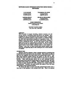
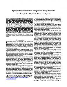
In today’s world, many people own and carry GPS-enabled mobile phones. Due to the e911 mandate, wireless carriers must be able to locate a 911 mobile-phone caller to within 50 to 300 meters of accuracy (3). Various technologies have been used to satisfy this mandate including embedded GPS hardware in mobile phones. The implementation of such positioning technologies has also led to the creation of a class of software application known as Location-Based Services (LBS) that use the device’s location in coordination with other data to create location-aware applications. Location-aware applications are the focus of several research projects at the Center for Urban Transportation Research and the Department of Computer Science and Engineering at the University of South Florida. One particular project, TRAC-IT, is a group of software applications used to monitor and analyze travel behavior using GPS data gathered from GPSenabled mobile phones (4). The primary data collection software is a Java Micro Edition (Java ME) application that runs in real-time on the user’s mobile phone, requiring no special hardware device for GPS data collection. Therefore, TRAC-IT can be carried with the participant on all modes of transportation and can record user-specific travel behavior. Even if a mobile phone is shared within the same household, the TRAC-IT software allows users to log-in with their own unique account so that collected data is attributed to the correct user. The travel behavior data collected using TRAC-IT can be utilized for many different purposes such as travel demand models for policymakers and transportation professionals or real-time traffic information services for the user. While GPS data is collected passively from the mobile phone, the TRAC-IT application user interface can also actively collect other trip information not directly recorded by GPS alone such as trip purpose, mode of transportation, and vehicle occupancy. This raises accuracy concerns as with other travel surveys that rely on participant’s input. The burden of repeated manual data entry may cause participant fatigue and result in individuals dropping out of the survey. For these reasons, it is desirable to automatically derive as many trip attributes as possible, directly from the GPS data to eliminate the need for active user input. Many difficulties are encountered when attempting to automate mode detection. Buses and cars tend to display similar attributes as seen in Figures 1 and 2. When comparing walking to other modes of transportation; the difference is noticeable as shown in Figure 3. Noteworthy here is that the walking trip is shorter than the other two trips, and less distance is traveled between the two GPS fixes. Software applications can be programmed to differentiate a walking trip from a car or a bus trip. However, this is not the case when distinguishing a car trip from a bus trip. The distance traveled in the bus trip (Figure 1) is approximately the same as that traveled by car (Figure 2) and the distance between the two GPS fixes is almost identical. Due to these and other similarities between car and bus trips, determining whether the trip mode is a car or a bus becomes rather challenging. Geographic Information Systems (GIS) data showing bus stops or routes can be utilized to determine whether the trip was taken by car or bus. GIS data from certain transit agencies may not be available in a consistent format or may be out of date. Since the utility of mode identification techniques rely on specifically formatted GIS data from transit agencies and since specialized GIS software is limited, expensive, and requires specific expertise to use and maintain, it is therefore advisable to find others means for mode detection techniques independent of GIS.
-2-
Figure 2 - GPS Data of Car Trip
Figure 1 - GPS Data of Bus Trip
Figure 3 - GPS Data of Walking Trip
This paper examines the feasibility of using neural networks to automatically detect the mode of transportation from assisted GPS data collected using actual GPS-enabled mobile phones through the standardized application programming interface (API) for Java-enabled mobile devices, the JSR179 Location API (5). This study also explores how this method can be modified to detect the mode of transportation by examining only critical points, (a minimum set of GPS fixes required to accurately reconstruct the user’s path) (7). Successful mode detection utilizing fewer GPS data points enables the TRAC-IT mobile application to transmit fewer GPS fixes to a server, thereby saving costs incurred for data transfer as well as devices and network resources including battery energy, network bandwidth, and required storage space.
RELATED WORK Previous research has examined the use of a neural network in automatic mode detection such as work by Byon et al. (6). However, that study used surrogate GPS data collected using stand-alone GPS units tethered to a laptop. While Byon’s research is informative for general strategies for mode detection using neural networks, it fails to accurately reflect the feasibility of mode detection using GPS data from mobile phones. Since characteristics of assisted GPS technology used in GPS-enabled mobile phones include increased sensitivity and a reduced time-to-first-fix, mobile phones can yield location data that is significantly different than data generated by traditional stand-alone GPS devices. Neural network performance is dependent on the characteristics of input data, therefore, mode detection using assisted GPS data from GPS-enabled mobile phones must be analyzed. Byon’s research used attributes of GPS data such as instantaneous acceleration and horizontal dilution of precision (HDOP), properties which are not accessible through the standardized application programming interface (API) implemented in most GPS-enabled mobile phones, the JSR179 Location API (5). Therefore, new data attributes that are available in assisted GPS data obtained through the JSR179 Location API must be substituted as potential neural network inputs. -3-
Byon et al. also examines how the frequency of location updates from the mobile phone impact the accuracy of mode detection. It is best to maximize the interval of time between location updates to minimize the impact on battery energy, along with data and financial costs incurred for every transferred GPS fix. In their research, Byon et al. assumed that the frequency is a static, fixed interval that cannot be dynamically modified, and that the cellular network controls the frequency of position updates. However, a Java ME application running on the mobile phone and utilizing the JSR179 Location API is capable of intelligently filtering location data using a critical point algorithm to send only GPS fixes that are required to reconstruct an accurate representation of the user’s path to a server (7). The critical point method differs from a fixed update interval in that the fixed update interval will always report a position every X seconds, even if that position information does not contribute to the knowledge of the user’s path (Figure 4). The Critical Point algorithm provides a dynamic update method without a fixed location update interval, and is capable of providing GPS data points collected at strategic locations of the path instead of random locations governed by a static update interval. Figure 5 shows all GPS data points collected during a car Figure 4 - The Critical Point Update Method Prevents Non-Critical GPS trip, while Figure 6 shows the remaining GPS data points Fixes From Being Sent to the Server. for the same trip after applying the critical point algorithm. This paper focuses on evaluating mode detection with a neural network on the basic case of entering all collected assisted GPS data, and also evaluates the feasibility of mode detection based on a minimum set of GPS fixes collected by using the Critical Point algorithm to filter out non-critical data points and save significant device resources during data collection.
Figure 5 - Car Trip All GPS Points
Figure 6 - Car trip Only Critical Points
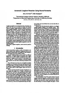
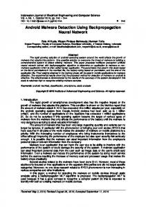
METHODOLOGY A neural network called a Multi-Layer Perceptron was used for the research presented in this paper. Neural networks can extract subtle information from data that is often missed by humans or other analysis algorithms (8). A neural network takes a series of inputs, processes them through hidden nodes and then generates an output that classifies the input data (Figure 7). During the training of the neural network, the calculated output is compared to the known correct output for the training data set being used. If the neural network’s output for the test data is incorrect, the weights between the input nodes, hidden layer nodes, and output nodes are adjusted accordingly in a method known as “back propagation”. The training process is repeated until the accuracy of the network reaches a threshold defined by the user, or until a certain number of training iterations known as “epochs”, are completed. The weights, which represent the trained neural network, are then used by the network to evaluate future data for which the correct output is not known. Various settings for the neural network model can be adjusted to affect the training process including hidden layers, the number of nodes in hidden -4-
layers, the rate at which the weights are adjusted (i.e., the learning rate), and the amount of training. The ability of a neural network to generalize conclusions for data which do not exactly match the training data is one of the significant strengths of this type of artificial intelligence. Based on the chosen neural network settings and input data attributes, the neural network can learn the subtle differences between car, bus, and walking trips and, therefore, automatically detect the mode of transportation for a new, previously unseen trip.
Figure 7 - Neural Network Topology for Mode Detection
An open-source Java application that supports a variety of knowledge discovery functions, Weka, was used to determine the feasibility of automating mode detection through the use of neural networks and assisted GPS data (9). A Multi-Layer Perceptron is programmatically created with particular settings that are further discussed in the Performance Evaluation section. After the neural network is created, the inputs for each GPS trip are calculated and fed into the neural network. Once the inputs are calculated and entered, a 10-fold crossvalidation is performed to train and test the neural network. The N-fold cross-validation randomly partitions a set of data with known correct outputs into N folds, and then utilizes one fold as a testing data set while the remaining N-1 folds are used as the training data set (10). This process is repeated N times with a different fold being used as the testing data for each iteration. The resulting N accuracy measurements taken from the testing data sets are averaged to provide a realistic performance measure of accuracy. Once the 10-fold crossvalidation is finished, the neural network outputs a trained model and the average accuracy of correctly identified modes from the testing data sets. Since the neural network is completely dependent on the training data set to learn to distinguish modes of transportation, it is important to examine the inputs that are entered. The next two sections discuss the attributes input data for the neural network when all GPS points for a trip are used for mode detection, and the attributes used when only critical points are used for mode detection. Neural Network Input for Mode Detection Using All GPS Points For data evaluated in this research, the GPS-enabled mobile phone was programmed to recalculate a new position every four seconds. The following data attributes were used as inputs to the neural network for a particular trip when using all of the GPS coordinates as input to the network: • • • • • •
Average Speed Maximum Speed Estimated Horizontal Accuracy Uncertainty Percent Cell-ID Fixes Standard Deviation of Distances Between Stop Locations Average Dwell Time -5-
It is desirable to select GPS data attributes with clear differences between modes to allow the neural network to easily identify a particular mode. The average speed and the maximum speed were chosen as inputs since different modes of transportations will exert different average and maximum speeds. For example, the maximum speed of a car can be 80 miles per hour, whereas a bus will not likely reach that speed. The estimated horizontal accuracy uncertainty is a measurement of the estimated confidence that the mobile phone places in a calculated GPS position. This value was chosen as an input since different modes of transportation have different values for estimated horizontal accuracy uncertainty. For example, a bus has the worst estimated horizontal accuracy uncertainty since it is essentially a metal box that obstructs the GPS signals. Conversely, a walking trip has the best estimated horizontal accuracy uncertainty since typical GPS signal obstruction is caused by a bag or purse. Another important input for this algorithm is the percent Cell-ID fixes, which are the percentage of location fixes that refer to cellular signal coverage instead of the GPS position of the phone. Cell-ID location fixes are obtained by the mobile phone when it cannot calculate a GPS fix. This percentage also serves as a rough measure GPS signal quality. The standard deviation of distances between stop locations is also used as an input since different modes of transportation exhibit different types of values. For example, a bus trip is likely to travel less distance between stops than a car due to the repeated stops that a transit vehicle typically makes. Finally, the average dwell time is used as the last input. The average dwell time refers to the average length of time that a user is stopped each time their speed falls below a certain threshold. For example, the average dwell time is often higher for car trips or walking trips, and lower for bus trips since most buses make quick stops to allow riders to board or exit the vehicle. Neural Network Input for Mode Detection Using Critical Points Only As mentioned in the previous section, automated mode detection using only critical points is important since efficient, location-aware applications may only transfer critical points to a server for analysis. Therefore, most of the inputs mentioned in the previous algorithm cannot be used as there is not sufficient data to calculate the values when only critical points are available. For example, to calculate the accurate standard deviation of stops and the average dwell time, all of the GPS fixes are necessary. For this reason, different inputs to the neural network are required when only critical points for a trip are available. The following inputs are used for critical points: • • • • • • • •
Average Acceleration Maximum Acceleration Average Speed Maximum Speed Ratio of the number of critical points over the total distance of the trip Ratio of the number of critical points over the total time of the trip Total Distance Average distance between critical points
Two important inputs are the average and maximum acceleration of a trip. Byon et al. notes that acceleration is a key identifier of different types of modes, and therefore is a valuable attribute for automated mode detection (6). Since instantaneous acceleration is not directly -6-
exposed to the application by the JSR179 Location API, the average acceleration must be calculated by dividing the change of velocity by the change in time of two consecutive GPS points. However, calculating average acceleration poses a problem when using the traditional critical point algorithm since by definition critical points are not temporally or spatially near one another. Therefore, a modified version of the critical point algorithm was created that records the velocity and time value for the GPS point either immediately after, or immediately before the current critical point. Figure 8 and Figure 9 illustrate this concept.
Figure 8 - Critical Points for a Trip
Figure 9 - Two Velocity and Time Values per Critical Point
Having two velocity and time values per critical point allows the change of velocity and the change in time to be calculated to get the average acceleration for that time period. The maximum average acceleration can be selected from the set of average acceleration values. The set of average acceleration measurements can be added and divided by the number of measurements to calculate the average acceleration for the entire trip. It was concluded that recording the GPS fix immediately after the critical point was preferred over recording the fix immediately before the critical point, since positive acceleration values are preferred over deceleration. A traveler is most likely to decelerate just prior to the critical point fix, given that they may be changing directions. After the traveler makes the turn, the acceleration is more likely to be a higher positive value. This modified version of the critical point algorithm can be implemented so that the number of wireless transmissions to the server is not increased over the traditional algorithm. The transmission of a critical point can be delayed until the next GPS fix is calculated, and the velocity and time values for this second GPS fix can be packaged along with the critical point information that is then sent to the server. Similar to the method that uses all GPS fixes, the average and maximum speeds are important since different modes of transportation will exert different average and maximum speeds. The ratio of the number of critical points over the total distance of the trip is another important input since different transportation modes may have different ratio values. Table 1 shows the average number of critical points within the different modes of transportation collected by a sample of seven car, walking, and bus trips. As the table describes, car trips are likely to have the highest critical point count since cars are more likely to make turns in a given trip. The second highest is the walking trips, followed by the bus trips which show a fewer number of critical points. Taking the number of critical points of a trip and dividing it by the total distance of the trip shows a trend in ratios within the same transportation mode since the number of turns in relationship to the total distance tends to be unique within different modes of transportation. -7-
Table 1 - Number of Critical Points for a Sample Set of Trips
#CP per Trip Trip 1 Trip 2 Trip 3 Trip 4 Trip 5 Trip 6 Trip 7 Average
Car Walk
Bus
146 86 70 238 103 79 44 109
51 120 50 45 46 43 89 63
137 35 124 59 15 140 9 74
Ratio - Critical point number over Total trip distance 200 180 Ratio (Critical points/Miles)
Figure 10 shows the different ratio values for each transportation mode. A similar ratio, the number of critical points over the total time of the trip, is also used to train the neural network. Similarly, different ratio trends within the different transportation modes are seen in Figure 11. These two ratios may help the neural network to further learn the differences between car, bus, and walking trips.
160 140 120
Car
100
Walk Bus
80 60 40 20 0 1
2
3
4
5
6
7
Trip sample
Figure 10 - Number of Critical Points per Mile for Sample Trip Set Ratio - Critical points over total time 0.016 0.014 Ratio (Critical points/seconds)
Since car and bus trips are the most difficult to distinguish from one another, it is best to find GPS data attributes that are very different. One such input is the average distance (miles) between critical points (Figure 12). There are significant differences in the average of the distance between different modes of transportation and consistent differences between cars and buses. Buses tend to change their travel direction more often than cars and, therefore, less distance is covered between critical points, while walking trips change travel direction more frequently.
0.012 0.01 Car Walk
0.008
Bus 0.006 0.004 0.002 0 1
PERFORMANCE EVALUATION
2
3
4
5
6
7
Trip Sample
Figure 11 – Number of Critical Points per Second for Sample Trip Set Average Distance Between Critical Points 0.12 Average Distance between Critical Points (miles)
Finally, the total distance (miles) is another important input for the neural network. As previously mentioned, different modes have different trip distances. For example, a walking trip distance will rarely exceed three miles, whereas the majority of car or bus trips are often more than three miles.
0.1
0.08 Car
Walk 0.06 To train and test the Multi-Layer Perceptron using Bus 10-fold cross-validation, 114 trips were recorded 0.04 in the Tampa, Florida area using the TRAC-IT 0.02 Java ME application on Motorola i870 and i580 0 phones on the Sprint-Nextel iDEN network. 1 2 3 4 5 6 7 Assisted GPS data was gathered for 38 car, bus, Trip Sample and walking trips. Usually only critical points Figure 12 - Average Distance (miles) would be transferred from the mobile phone to a Between Critical Points server, but for these tests all GPS fixes were transferred to the server and the critical points algorithm was used to mark the critical points in the database during post-processing. This process allows either all GPS points, or critical points only to be input into the neural network for the exact same trip.
GPS data for the 114 trips is first extracted from the database server and written into Weka’s ARFF file format. This ARFF file is then read by Weka and input into its neural network function for training and testing purposes. For all tests, Weka’s auto-build feature was used
-8-
to create the neural network topology with a single hidden layer that consists of a particular number of nodes. The number of hidden nodes is determined by the following equation: Number of hidden nodes = (Number of attributes + Number of possible classifications) / 2 Since there are additional settings in the neural network that can be manipulated, it is important to evaluate the effect of different settings on the accuracy of mode detection. The following sections illustrate the possible performance gains from utilizing different neural network settings. Evaluation with Initial Settings In this section, the performance of the neural network with its default settings is evaluated on two different sets of trip data: all GPS points, and only critical points for a trip. The following are the initial neural network settings: • The learning rate is set to: 0.01 • The training time is set to: 100 epochs The learning rate is a number from 0 to 1 that is the amount the neural network weights are adjusted during each round of back-propagation. The training time specifies the number of training epochs that the neural network should perform. Table 2 displays the accuracy for mode detection using both types of inputs and the initial neural network settings.
Table 2 - Accuracy of Mode Detection Using 0.01 Learning Rate and 100 Epochs
Type of Input All GPS Points Only Critical Points
Accuracy 57.02% 62.29%
Exploring Different Settings Changing the Multi-Layer Perceptron’s settings helped improve the accuracy for mode detection. Table 3 describes the improvements changing the settings to the following: • The learning rate is set to: 0.1 • The training time is set to: 300 epochs Table 4 describes the change in accuracy changing the settings to the following:
Table 3 - Accuracy of Mode Detection with 0.1 Learning Rate and 300 Epochs
Type of Input All GPS Points Only Critical Points
Table 4 - Accuracy of Mode Detection with 0.3 Learning Rate and 300 Epochs
Type of Input All GPS Points Only Critical Points
• The learning rate is set to: 0.3 • The training time is set to: 300 Finally, Table 5 describes the change in accuracy changing the settings to the following:
-9-
Accuracy 85.97% 88.6%
Table 5 – Accuracy of Mode Detection with 0.3 Learning Rate and 500 Epochs
Type of Input All GPS Points Only Critical Points
• The learning rate is set to: 0.3 • The training time is set to: 500
Accuracy 88.6% 91.23%
Accuracy 85.09% 85.97%
As indicated by the tables, setting the learning rate and the training time to different values affects the accuracy for mode detection while using the same set of inputs. A learning rate increased to 300 epochs has the highest accuracy of 91.23% for Critical Points Only input. This indicates that the neural network benefits from additional training over 100 epochs, but over-training the network results in lesser performance. Additionally, using only critical points may further aid the network in successful classification by eliminating GPS data that does not contribute useful information about the mode of transportation. Correlation between Input Attributes and Mode Detection Accuracy This section explores how inputs in the algorithm using only critical points help the neural network to train for a high accuracy percentage on the testing set. The purpose is to see if the number of inputs for this algorithm can be limited so that noise that keeps the neural network from performing better can be eliminated. Table 6 describes the relationship between the type of input and the average accuracy of mode detection using only those inputs. The neural network settings found to be optimal in the previous section of a learning rate is a set of 0.1 and a training time of 300 are used. Table 6 shows how different inputs affect the accuracy of the neural network. Some inputs actually degrade accuracy instead of improving it. For example, the set of selected inputs in column F have an accuracy of 90 percent, but once the ratio of critical point number over total time is included as an input (column G), the accuracy decreases. A similar situation occurs between the inputs used in columns D and E. This reduction in accuracy when new inputs are added can be a result of input noise, which confuses the neural network instead of helping it learn. It is important to note that the highest accuracy (91.23%) was reached when utilizing all selected inputs. The second highest accuracy, 90.4 percent, is achieved when the ratio of critical point number over total time is removed from the input data set. Table 6 - Accuracy of Mode Detection When Using Different Combinations of Data Attributes as Neural Network Inputs
Max. Speed Avg. Speed Max. Acceleration
A X X X
Avg. Acceleration
X
# CP over Total distance
B X
C X
D X
X
X
X
E X X X
F X
G X
X
X
X
X
X X
X
X
# CP over Total time Total Distance Avg. Dis. between CP Average Accuracy (%)
X
86
X 86
X 85.1
-10-
X
X
87.7
86.9
X X 90.4
X X 89.4
Table 7 – Accuracy of Mode Detection
Table 7 shows the accuracy achieved for each for each Mode of Transportation individual mode of transportation for the highest Mode of Average Accuracy overall mode detection accuracy of 91.23 percent. Transportation Per Mode These results are important since they demonstrate Car 92.11% that bus trips are suffering from the highest number Bus 81.58% of incorrect classifications, at 18.42 percent. The car Walk 100.0% mode follows with 7.89 percent of trips classified incorrectly. It is clear that the neural network easily differentiates walking trips since none were incorrectly classified. For future research, efforts will focus on finding additional inputs to better differentiate bus from car trips. As is evident from the results presented, selecting a proper set of inputs for the neural network and maximizing the accuracy obtained with those inputs requires some experimentation. CONCLUSION Next-generation transportation surveys will utilize GPS to collect trip data. Due to their ubiquity, GPS-enabled mobile devices are promising survey tools. As demonstrated in this research paper, automatic mode detection was possible when utilizing a neural network and assisted GPS data collected via GPS-enabled mobile phones. Furthermore, mode detection accuracy was actually improved when only a small subset of GPS coordinates required to build the user’s path (i.e., critical points) are used as neural network input. Using only critical points allows a mobile phone application to reduce the number of GPS fixes that are sent to a server for analysis, thereby saving battery energy, network bandwidth, and storage space. However, a new set of data attributes for neural network input had to be developed for the critical points-only datasets since the reduction in available GPS data makes the calculation of some attribute used for the full GPS datasets impossible. The highest accuracy accomplished for mode detection using 10-fold cross-validation was 91.23 percent for the critical points-only dataset and a neural network learning rate of 0.1 and training time of 300 epochs. When broken down by mode, the neural network correctly predicted 92.11 percent of the car trips, 81.58 percent of the bus trips, and 100 percent of the walking trips for this test series. Future efforts will focus in trying to identify additional data attributes that better differentiate car trips from bus trips. ACKNOWLEDGEMENTS This work was supported in part by the National Science Foundation under grant No. 0453463, the Florida Department of Transportation, and the United States Department of Transportation through the National Center for Transit Research under grant numbers BD549-24 “Testing the Impact of Personalized Feedback on Household Travel Behavior (TRAC-IT Phase 2)” and BD-549-35 “Smart Phone Application to Influence Travel Behavior (TRAC-IT Phase 3)”. REFERENCES (1) Murakami, E., Wagner, D. P., Neumeister, D. M. (1997) “Using Global Positioning Systems and Personal Digital Assistants for Personal Travel Surveys in the United States,” International Conference on Transport Survey Quality and Innovation, -11-
Grainau, Germany. http://gulliver.trb.org/publications/circulars/ec008/session_b.pdf, July 2004. (2) Murakami, E.and D. P.Wagner. (1999) Can using global positioning system (GPS) improve trip reporting? Transportation Research Part C, 7(2/3):149-165. (3) Federal Communication Commission (FCC). “Enhance 911 – Wireless Services.” Accessed online 10/8/2006 at http://www.fcc.gov/911/enhanced/, accessed June 26, 2008. (4) Winters, Philip; Barbeau, Sean; and Georggi, Nevine, (2008). Smart Phone Applications to Influence Travel Behavior (TRAC-IT Phase 3). National Center for Transit Research. University of South Florida. Florida Department of Transportation http://www.nctr.usf.edu/pdf/77709.pdf, accessed June 26, 2008. (5) Sun Microsystems, Inc. “Java Specification Request (JSR) 179: Location API for J2ME™,” http://jcp.org/en/jsr/detail?id=179, accessed June 26, 2008 © Sun Microsystems, Inc. 2007. (6) Byon, Y. and Abdulhai, B. “Impact of Sampling Rate of GPS-enabled Cell Phones on Mode Detection and GIS Map Matching Performance,” Transportation Research Board Annual Meeting 2007 Paper #07-1795. (7) Barbeau, S., Labrador, M., Perez, A., Winters, P., Georggi, N., Aguilar, D., Perez, R. “Dynamic Management of Real-Time Location Data on GPS-enabled Mobile Phones,” UBICOMM 2008 – The Second International Conference on Mobile Ubiquitous Computing, Systems, Services, and Technologies, Valencia, Spain, September 29 – October 4, 2008. (8) Haykin, Simon. Neural Networks: A Comprehensive Foundation, 2nd Edition. Prentice Hall, 1998. (9) University of Waikato. “Weka 3: Data Mining Software in Java,” http://www.cs.waikato.ac.nz/ml/weka/, accessed June 26, 2008. (10) Kohavi, Ron. “A study of cross-validation and bootstrap for accuracy estimation and model selection”. Proceedings of the Fourteenth International Joint Conference on Artificial Intelligene. August, 1995.
-12-