Comment on ”Efficient Line Search Methods For Convex Functions”
H. Alipour1 , K. Mirnia Faculty of Mathematical Science, University of Tabriz, Tabriz-Iran
Abstract In this paper, we point some problems about Improved Golden Section (IGS) method mentioned in ”Efficient Line Search Methods For Convex Functions” in [2]. We show that this method, contrary to the claim of the authors, is not better than Regular Golden Section (RGS) method. We also present three new algorithms and compare them with RGS and IGS showing no efficient of IGS comparing with RGS. K eywords: Convex Function, Unimodal, Line Search, Golden Section.
1
Introduction
It is expected that when a new algorithm is proposed for a set of problems, it should have better performance comparing to former algorithms. When using RGS algorithm, the interval of uncertainty is reduced by a factor 0.618t−1 after t function evaluations and algorithm terminates after at most 1+(
0 log( b0 −a ε ) ) 1 log( 0.618 )
(1)
function evaluations, where a0 and b0 are the corresponding end points of initial interval containing optimal point and ε is the final interval length [3]. This paper is organized as follows. In section (2) we compare IGS algorithm mentioned in [2] with RGS algorithm. We also present a new algorithm that uses the convexity property and also it is compared with IGS. In section (3) we present two new algorithms that use the convexity and golden section properties and compare them with other algorithms presented in this paper. The numerical results are presented in section (4). Section (5) summarizes the discussions.
2
Comparison between IGS and RGS algorithms
In this paper we assume that the optimal point of convex function occurs at an inner point of the interval [L,U] (otherwise we use algorithm (2) from [2] until optimal point occurs at an inner piont). By supposing the availability of the function values at boundaries of the initial interval, RGS starts. It uses unimodality and convexity characteristics to obtain an interval that contains 1
Corresponding author, Email:
[email protected]
1
minimum point of convex functions. At each iteration of RGS algorithm, we just have one function evaluation(except at the beginning of the algorithm where two function evaluations are required) and one comparison between function values at two points, and the interval of uncertainty is reduced by a factor 0.618. Thus after t function evaluations, the interval of uncertainty is reduced by a factor 0.618t−1 . We recall here the strategy in [2] claiming that is an improved version of the RGS algorithm: ”Let f (x) be a continuous, univariate, convex function on a closed domain D. Assume that for a given set of points χ = {x1 , ..., xn } in D the function values of f are known.
Fig. 1. (a) Example of a convex function f with six function evaluations. (b) A piecewiselinear upper bound based on the convexity property. (c) A piecewise-linear lower bound based on the convexity property. (d) (Magnified in comparison with (a)-(c).) The optimum lies somewhere in the gray areas, the areas of uncertainty. The interval of uncertainty based on the convexity property is given by [L,U].
Fig. 2. Example where the golden section method chooses a point outside the interval of uncertainty for function evaluation. Five function evaluations have already been made following the sequence A, . . . , E. The sixth point for evaluation proposed by golden section is point F. However, the interval of uncertainty comprising the two small gray triangles is located to the right of F.
Figure 1(a) gives an example of a convex function f of which six function evaluations are known. As f is convex, αf (xi ) + (1 − α)f (xj ) ≥ f (αxi + (1 − α)xj ) with α ∈ [0, 1] for each xi , xj ∈ χ. Using this property we obtain the piecewise-linear upper bound f u of f with f u (x) ≥ f (x) for all x ∈ D and f u (x) = f (x) if x ∈ X; cf. Figure 1(b). Now we consider the line segments BC and DE and extend them until they intersect at point K, as shown in Figure 2
1(c). Then, the lines CK and KD give a lower bound for the function f between x3 and x4 . This can be done for any four consecutive points, resulting in the lower bound f l on f given in Figure 1(c) by the dashed line. Now let xk ∈ χ be a point with the lowest determined function evaluation, i.e., f (xk ) ≤ f (x) for all x ∈ χ. Then the minimum function value of f must lie between f (xk ) and the minimum of f l (x). The possible locations of the minimum are given in Figure 1(d) by the gray areas, the areas of uncertainty. The interval of uncertainty is [L, U ]. This shows how the interval of uncertainty can be decreased using the convexity property. The next step in finding the minimum of f is to choose a point for evaluation. Naturally, this should be a point in the interval of uncertainty. Taking one of the existing methods to choose a point, however, does not always give a point in the interval of uncertainty. Figures 2 shows an example where the golden section method would evaluate the function at a point that is outside the interval of uncertainty.” At this stage, we mention that: (i) This strategy works when the function values are known in at least four points, otherwise, the uncertainty interval can not be determined. (ii) To determine the interval of uncertainty, we have to obtain intersection points between line f (xk ) = min{f (xi ), xi ∈ χ} and function f l . Note that in RGS, we don’t need any computations expressed in (ii). In comparison to (i), at each iteration, we just need to have function values at four points: We have three function values from previous iteration and in current iteration we need to compute function value just at one new point. But in (i) we don’t know how many function values can be used for the next iteration and how many times the function must be computed, but it is clear that the amount of computations are more than RGS. Now, we recall the second strategy that is used in [2]: ”IGS method starts in the same way as the RGS method. Let [L, U ] be the interval of uncertainty with two inner points x1 and x2 such that x2 − L = U − x1 = τ (U − L). Now we assume that x1 has the lowest function value, i.e., f (x1 ) ≤ f (x2 ); if f (x2 ) < f (x1 ) , then we can follow a strategy analogous to what we describe as follows. The new interval of uncertainty using the RGS method is now given by [L, x2 ]. Using the convexity property we can obtain a smaller interval of uncertainty [L0 , U 0 ] for which L0 ≥ L and U 0 ≤ x2 . Now we assume that x1 is an interior point of [L0 , U 0 ]. The RGS method would choose a new point x3 = x2 − τ (x2 − L) so that x2 − x3 = x1 − L. However, if we replace [L, x2 ] by [L0 , U 0 ] and then choose x3 = U 0 − τ (U 0 − L0 ), U 0 − x3 is generally not equal to x1 − L0 , meaning that the two interior points x1 and x3 do not satisfy the golden section property w.r.t. the interval of uncertainty [L0 , U 0 ]. Therefore, we will stretch the ˜ U ˜ ] such that the golden section property can be maintained interval [L0 , U 0 ] to a new interval [L, for the new point to be evaluated. We distinguish four possibilities for this (a) x1 ≤ U 0 − τ (U 0 − L0 ), (b) U 0 − τ (U 0 − L0 ) < x1 < 12 (U 0 + L0 ), (c) 12 (U 0 + L0 ) ≤ x1 < L0 + τ (U 0 − L0 ), (d) x1 ≥ L0 + τ (U 0 − L0 ). The corresponding stretched intervals are the following
3
(2)
(a) (b) (c) (d)
˜ = U 0 − 1 (U 0 − x1 ), L τ ˜ = L0 , L ˜ = 1 (x1 − τ L0 ), L 1−τ ˜ = L0 , L
˜ U ˜ U ˜ U ˜ U
= U 0, 1 = 1−τ (x1 − τ L0 ), = U 0, = L0 + τ1 (x1 − L0 ),
(3)
By this strategy the obtained stretched interval is not larger than the interval of uncertainty ˜ U ˜ ] determined as described obtained with the RGS method.When the stretched interval [L, above, choose the new point x3 for function evaluation as follows for the four previously distinguished possibilities (a) (b) (c) (d)
x3 x3 x3 x3
˜ + τ (U ˜ − L) ˜ = U 0 − τ (U 0 − x1 ). =L ˜ + τ (U ˜ − L) ˜ = 1 x1 − τ L0 . =L τ ˜ − τ (U ˜ − L) ˜ = 1 x1 − τ U 0 . =U τ ˜ − τ (U ˜ − L) ˜ = L0 + τ (x1 − L0 ). =U
(4)
By this strategy, IGS algorithm performs at least as well as the regular golden section ˜ −L ˜ ≤ τ (U − L), while ensuring that the new point chosen for function method, means U evaluation lies in the interval of uncertainty.” At this stage, we follow: ˜ U ˜ ] such that the golden section property • Stretching the interval [L0 , U 0 ] to a new interval [L, can be maintained for the new point to be evaluated. At this part, we have the comparisons for checking the possible cases (2) and we have two evaluations corresponding to (3), (4). Now we note that the main goal in RGS and Fibonacci searches for choosing x3 = x2 − τ (x2 − L) so that x2 − x3 = x1 − L, is to obtain the best reduction in the interval of uncertainty with the least computations [1]. But in the second strategy of IGS, the computations are expensive and in addition, the uncertainty interval obtained from the first strategy should be stretched to obtain the golden section property but this destroys the first strategy. Thus it is expected that the uncertainty interval obtained from IGS is not so smaller than that obtained from RGS. To save the length of uncertainty interval obtained from first strategy, we can use easier strategy instead of second 0 1 strategy for choosing new point x3 . For example we can choose x3 = L +x if f (x1 ) ≤ f (x2 ) or 2 0 x2 +U x3 = 2 if f (x1 ) > f (x2 ). We call this as the Convexity Property algorithm and denote it by CP. This algorithm doesn’t save golden section property but saves the convexity property used in the first strategy in IGS. So we expect that CP should work as good as IGS. If the number of points used at each iteration are more than four, then decreasing the uncertainty interval can be remarkable. But execution time needed for computations will be increased by increasing the number of points. Moreover, there is no strategy for choosing the new points for the next iteration, because the second strategy tries to save the Golden Section property working with four points. Thus to compare between IGS and GS, we apply the IGS with four points at each iteration.
4
3
Two new algorithms that use the convexity and golden section properties to reduce the interval of uncertainty
3.1
Improved CP algorithm (ICP)
In the previous section, we presented CP to save the length of uncertainty interval obtained from the first strategy. Now we can improve the first strategy instead of saving it in case f (x1 ) = f (x2 ) as follows: In this case we set L0 = x1 , U 0 = x2 instead of using convexity property. Then, instead of the second strategy we choose two new inner points x3 and x4 satisfying in the golden section property. Otherwise apply CP. We call this Improved CP algorithm denoting it by ICP. Computations for this algorithm are almost equal to CP but the length of uncertainty interval obtained from ICP is less or equal to that obtained fromCP. So it is expected that this algorithm should work better than CP. But since the computations in ICP are more than RGS, we expect RGS to be better than ICP.
3.2
Improved IGS algorithm (IIGS )
Now we can use golden section property and convexity property more efficiently in our algorithm as follows: 1: Instead of using first strategy in IGS we set L0 = x1 , U 0 = x2 if f (x1 ) = f (x2 ), otherwise the first strategy in IGS is applied. 2: Instead of choosing one new inner point, we can choose two new inner points in the uncertainty interval obtained from the previous strategy satisfying in the golden section property. We call this as Improved IGS algorithm and denote it by IIGS. Computations for this algorithm are almost equal to IGS but the length of uncertainty interval obtained from IIGS is less or equal to that obtained from IGS. So it is expected to be better than IGS. But since the computations for IIGS are more than RGS, we expect RGS still be better than IIGS.
4
Numerical results for RGS, IGS, CP, ICP and IIGS algorithms
In this section, we compare RGS, IGS, CP, ICP and IIGS algorithms. For these algorithms, we start with four points L, x1 , X2 , U in the first interval [L,U] satisfying in the golden section property. Here ”N” denotes the number of iterations, ”L-U” denotes the length of uncertainty interval after N iterations and ”Time” denotes running time.
5
Table 1: f (x) = x2 in [-1,1]
RGS N
L-U
1 1.2361 2 0.7639 3 0.4721 4 0.2918 5 0.1803 6 0.1115 12 0.0062 36 5.9e − 8 37 3.7e − 8 80 3e − 17
IGS Time
L-U
0.002 0.7639 0.002 0.4721 0.003 0.2918 0.003 0.1803 0.004 0.1115 0.004 0.0689 0.007 0.0038 0.017 3.7e − 8 0.017 2.2e − 8 0.04 2e − 17
CP Time
L-U
0.002 1.2361 0.003 0.6525 0.004 0.3867 0.004 0.2293 0.005 0.1289 0.006 0.0764 0.010 0.0028 0.03 5.3e − 9 0.03 2.9e − 9 0.07 1 − 019
ICP Time
L-U
0.002 0.4721 0.003 0.1115 0.004 0.0263 0.004 0.0062 0.005 0.0015 0.006 3.4e − 4 0.010 5.9e − 8 0.03 5e − 23 0.03 1e − 23 0.07 1e − 50
IIGS Time
L-U
0.003 0.4721 0.003 0.1115 0.004 0.0263 0.004 0.0062 0.005 0.0015 0.006 3.4e − 4 0.014 5.9e − 8 0.03 5e − 23 0.03 1e − 23 0.07 1e − 50
Time 0.002 0.003 0.004 0.004 0.005 0.006 0.011 0.03 0.03 0.07
Table 2: f (x) = x2 in [-2,1]
RGS N
L-U
1 1.8541 2 1.1459 3 0.7082 4 0.4377 5 0.2705 6 0.1672 7 0.1033 12 0.0093 13 0.0058 37 5.5e − 8 38 3.4e − 8 80 5e − 17
IGS Time
L-U
0.002 1.8541 0.002 1.1459 0.003 0.7082 0.003 0.4377 0.003 0.2705 0.004 0.1672 0.004 0.1033 0.006 0.0093 0.006 0.0058 0.015 5.5e − 8 0.015 3.4e − 8 0.03 5e − 17
CP Time
L-U
0.002 1.6060 0.003 0.9201 0.004 0.5679 0.004 0.4245 0.005 0.2460 0.006 0.1631 0.006 0.0933 0.010 0.0086 0.011 0.0052 0.03 4.6e − 8 0.03 3.0e − 8 0.06 6e − 17
6
ICP Time
L-U
0.002 1.6060 0.003 0.9201 0.004 0.5079 0.005 0.4245 0.005 0.2460 0.006 0.1631 0.007 0.0930 0.010 0.0086 0.011 0.0052 0.03 4.6e − 8 0.03 3.0e − 8 0.06 6e − 17
IIGS Time
L-U
0.002 1.6060 0.003 0.8848 0.004 0.4687 0.004 0.2636 0.005 0.1371 0.006 0.0811 0.006 0.0410 0.010 0.0021 0.011 0.0011 0.03 5.3e − 10 0.03 2e − 10 0.06 2e − 21
Time 0.002 0.003 0.004 0.004 0.005 0.006 0.007 0.010 0.011 0.03 0.03 0.6
Table 3: f (x) = (0.5(1 − x)2 + log(11 + x) + 1.5x + 0.75x2 )2 in [-4,4]
RGS
IGS
CP
ICP
N
L-U
Time
L-U
Time
L-U
Time
L-U
1 2 3 4 5 6 7 12 13 30 31 37 38 80
4.9443 3.0557 1.8885 1.1672 0.7214 0.4458 0.2755 0.0248 0.0154 4.2e − 6 2.6e − 6 1.4e − 7 9.1e − 8 1e − 16
0.004 0.004 0.004 0.006 0.006 0.007 0.007 0.012 0.015 0.023 0.024 0.028 0.028 0.06
4.9443 3.0557 1.8885 1.1672 0.7214 0.4458 0.2755 0.0248 0.0154 4.2e − 6 2.6e − 6 1.4e − 7 9.1e − 8 non
0.004 0.005 0.006 0.007 0.010 0.011 0.012 0.023 0.025 0.04 0.04 0.05 0.06
4.8998 3.0541 1.7431 1.1004 0.8103 0.4914 0.3220 0.0216 0.0162 3.3e − 6 2.2e − 6 1.1e − 7 7.1e − 8 non
0.004 0.005 0.006 0.007 0.010 0.011 0.012 0.020 0.022 0.04 0.04 0.05 0.06
4.8998 3.0541 1.7431 1.1004 0.8103 0.4914 0.3220 0.0216 0.0162 3.3e − 6 2.2e − 6 1.1e − 7 7.1e − 8 non
IIGS Time
L-U
0.004 4.8998 0.005 2.8192 0.006 1.6416 0.007 0.8970 0.010 0.5206 0.011 0.2681 0.012 0.1615 0.023 0.0071 0.025 0.0040 0.04 1.3e − 7 0.04 7.6e − 8 0.05 non 0.06 non non
Time
0.003 0.005 0.006 0.007 0.009 0.010 0.012 0.019 0.020 0.043 0.044
In Table 1, since the case f (x1 ) = f (x2 ) occurs in more iterations and obtaining the function values are not expensive, ICP and IIGS work better than RGS but IGS and CP are worser than RGS. Also, the results for ICP and IIGS are equal and CP works a little better than IGS for larger N. In Table 2, since the case f (x1 ) = f (x2 ) doesn’t occur more often iterations, RGS works better than IGS, CP, ICP and IIGS. There is no remarkable difference among IGS, CP and ICP but IIGS works a little better than them. In Table 3, the case f (x1 ) = f (x2 ) doesn’t occur for more iterations and since computing function values are expensive, hence RGS works so better than IGS, CP, ICP and IIGS. Again there is no remarkable difference among IGS, CP and ICP but IIGS works a little better than them.
5
Conclusions
From the previous discussions we conclude that RGS is better than IGS and CP. Also since the possibility of occurence the case f (x1 ) = f (x2 ) with inexpensive computing the function are less often, RGS works better than ICP and IIGS so for most examples. Hence the RGS is still better than ICP and IIGS. These results show that the RGS algorithm is better than IGS and the three new algorithms presented here show that there is a significant gap between the RGS and IGS algorithms.
7
References [1]
B. D. Bunday, Basic Optimisation Methods, Edward Arnold (Pub) Ltd, London 1984, pp. 13-19.
[2]
E. Den Boef, D. Den Hertog, Efficient Line Search Methods For Convex Functions, SIAM Journal on Optimization. Vol. 18. No. 1, pp. 338-363.
[3]
E. de Klerk et al. Optimization (WI4 207), Delft University of Technology, 2005, pp. 66-68.
8