$-\nabla p+\theta$$\hat{i}+\nabla^{2}u$ , ... $\partial_{t}\nabla^{2}\triangle_{2}\tilde{\phi}+\{U_{B}(z)\partial_{x}-\nabla^{2}\}\nabla^{2}\triangle_{2 ... $\overline{\psi}=\sum_{\mathrm{e}ll=0}^{\infty}\tilde{b}\iota(1-z^{2})T_{l}(z)\exp\{\mathrm{i}\alpha ...
数理解析研究所講究録 1454 巻 2005 年 161-166
161
鉛直チャンネル中の自然対流におけるスパン方向運動量生成について 板野智昭 (Tomoaki Itano), 中村亮介 (Ryosuke Nakamura), 永田 雅人 (Masato Nagata)
京都大学・工学研究科
Graduate School of Engineering, Kyoto University 概要
We investigate the bifurcation of three-dimensional tertiary flows numerically in a simple shear layer with a cubic velocity profile when secondary flow loses its stability to oscillatory perturbations. It is found that the bifurcating motion is either of periodic nature or of traveling-wave nature, depending on the spanwise symm etry of disturbances. Furthermore, it turns out that the travellingwave propagating in the spanwise direction generates tl le spanwise mean flow
1
Introduction
It is of considerable importance to applications in engineering and geophysics, among to under stand the mech anism of the transition from laminar flow to early stages of turbulence in plane parallel shear layers. As a simple example of such shear layers we consider flows with a cubic velocity profile. These flows with an inflectional velocity profile can be realized between two parallel vertical plates which are kept at constant different temperatures under the gravity field. The flows are characterised by a upward motion near a hotter plate and by a downward motion near a colder plate, so that the momentum for the undisturbed state is only in the vertical direction. It is well known that Squire’s theorem is applicable in this case, so that it is sufficient to analyse the stability of the basic state with respect to two-dimensional spanwise-independent) perturbations In fact, a spanwise-independent secondary flow characterized by cats’ eyelike transverse vortices sets in as the shear gets stronger (Vest &Arpaci ). The stability analysis on the secondary flow indicates that the secondary flow becomes unstable to threedimensional perturbations with either a monotone subh armonic nature or an oscillatory harmonic nature (Nagata &Busse ), In the present paper we investigate the nonlinear development of the perturbations in the oscillatory harmonic case using two numerical schemes: a direct numerical simulation to integrate the time evolution of the primitive variables for Navier-Stokes equations and a Newton-Raphson iterative scheme to solve the nonlinear algebraic equations for the disturbance amplitudes in an equilibrium state. $\mathrm{o}\mathrm{t}\mathrm{h}\mathrm{e}\mathrm{r}\mathrm{S}_{\rangle}$
$\mathrm{n}\mathrm{t}$
2
Mathematical formulation
162
$\mathrm{T}^{2}=\mathrm{T}-$
$\mathrm{T}^{*}=\mathrm{T}+$
$\xi$
$1$
$\mathrm{g}$
$\ovalbox{\tt\small REJECT}_{1}|_{\oint}||$
$\mathrm{z}^{*}=- \mathrm{d}|$
$\dot{\mathrm{z}=}0|$
$\mathrm{z}^{*}=+\mathrm{d}|$
$1$
$\mathrm{H}$
: Configuration
in (1) is the Grashof number defined by $G_{r}=\gamma gd^{3}(T_{+}-T_{-})/(2\nu^{2})$ where is the coefficient of thermal expansion, is the kinematic viscosity and is the acceleration due to gravity. The equations which govern disturbances deviated from the basic state (1) are written by $G_{r}$
$\gamma$
$g$
$\nu$
$\partial_{t}u+$
$d_{t}’\theta+$
.
(2)
at
$=$
0,
$(u. \nabla)u$
$=$
$-\nabla p+\theta$$\hat{i}+\nabla^{2}u$
$\nabla$
$(u \cdot\nabla)\theta$
$=$
$\frac{1}{Pr}\nabla^{2}\theta$
(3)
,
(4)
,
where is the velocity disturbance, the pressure disturbance, the temperature disturbance, the Prandtl number. The no slip boundary condition and the fixed temperatures are plates: $u=0$ and at $z=\pm 1$ . $\theta$
$P$
$\mathrm{u}$
$Pr=\nu/\kappa$
$\mathrm{p}\mathrm{r}\mathrm{e}\mathrm{s}\mathrm{e}^{\backslash }\mathrm{r}\mathrm{i}\mathrm{b}\mathrm{e}A$
on the (5)
$\theta=0$
It may be easily found that temperature disturbnce becomes identically zero in the vanishing Prandtl number limit. The stability of the basic state is governed by (6)
,
$\partial_{t}\nabla^{2}\triangle_{2}\tilde{\phi}+\{U_{B}(z)\partial_{x}-\nabla^{2}\}\nabla^{2}\triangle_{2}\tilde{\phi}-U_{B}’(z)\partial_{x}\triangle_{2}\tilde{\phi}=0$
and $\partial_{C}\triangle_{2}\tilde{\psi}+\{U_{B}(z)\partial_{x}-\nabla^{2}\}\triangle_{2}\tilde{\psi}-U_{B}’(z)\partial_{y}\triangle_{2}\tilde{\phi}=0$
where
$\tilde{\phi}$
and
$\tilde{\psi}$
are the poloidal and toroidal components of an infinitesimal velocity perturbation $\tilde{u}=\nabla \mathrm{x}$
superimposed on the basic flows (1)
$\nabla \mathrm{x}$
$(\tilde{\phi}k)+\nabla \mathrm{x}$
$(\tilde{\psi}k)$
.
(7)
, $\overline{u}$
: (8)
183
We express
$\tilde{\phi}$
and
$\tilde{\psi}$
as
$\tilde{\phi}=\sum_{\ell=0}^{\infty}\tilde{a}_{l}(1-z^{2})^{2}T_{l}(z)\exp\{\mathrm{i}\mathrm{c}\mathrm{y}x+\mathrm{i}\beta y+\sigma t\}$
(9)
,
(10)
$\overline{\psi}=\sum_{\mathrm{e}ll=0}^{\infty}\tilde{b}\iota(1-z^{2})T_{l}(z)\exp\{\mathrm{i}\alpha x+\mathrm{i}\beta y+\sigma t\}_{?}$
a
where a and are the wavenumbers in the streamwise and the spanwise directions, respectively. is the r-th Chebyshev polynomial. In order to analyse the nonlinear development of the perturbation we consider a velocity deviation and the \^u from the laminar state and for convenience separate it into the average part residual , so that the total velocity is given by $T\ell(z)$
$\check{U}(z)i+\check{V}(z)j$
$u$
$\dot{u}$
(11)
$u=U(z)i+\check{V}(z)j+\check{u})$
where
$U(z)=U_{B}(z)+\check{U}$ $(z)$
The residual
tt
is further decomposed into the poloidal and toroidal parts:
$\check{u}=\nabla \mathrm{x}\nabla \mathrm{x}$
$(\phi k)+\nabla \mathrm{x}$
$(\psi k)$
.
(12)
The nonlinear state is governed by
$\partial_{t}\nabla^{2}\triangle_{2}\phi$
$\partial_{t}\triangle_{2}\psi$
$+$
$\{U(z)\partial_{x}-\nabla^{2}\}\nabla^{2}\triangle_{2}\phi-U’(z)\partial_{x}\triangle_{2}\phi$
$+$
$\check{V}(z)\partial_{y}\nabla^{2}\triangle_{2}\phi-\check{V}’(z)\partial_{y}\triangle_{2}\phi$
$+$
$\delta[(\check{u}\cdot\nabla)\check{u}]=0$
(13)
,
$+$
$\{U(z)\partial_{x}-\nabla^{2}\}\triangle_{2}\psi-U’(z)\partial_{y}\triangle_{2}\phi$
$+$
$\check{V}(z)\partial_{y}\triangle_{2}\psi+V’(z)\partial_{x}\triangle_{2}\phi \mathrm{v}$
$+$
$\epsilon[(\dot{u}.
\nabla)\overline{u}]=0$
(14)
,
,
(15)
,
(16)
$\check{U}^{Jl}+\partial_{z}\overline{\triangle_{2}\phi(\partial_{xz}^{2}\phi+\partial_{y}\psi)}=\partial_{\mathrm{g}}\check{U}$
$\dot{V}’+\partial_{z}\overline{\triangle_{2}\phi(\partial_{yz}^{2}\phi-\partial_{x}\psi)}=\partial_{t}\check{V}$
where the differential operators
$\epsilon$
in (11) and 6 in (12) are defined by
$\epsilon\equiv k(\nabla \mathrm{x}$
and
(17)
$\mathit{5}\equiv k(\nabla\cross\nabla \mathrm{x}.$
and the overline in (15) or (16) stands for the , -average. In the above, the possibility of induced and as follows: in the spanwise direction is incorporated. We express , average fiow $x$
$y$
$\phi$
$\check{V}(z)$
$\phi$
$\psi,\check{U}$
$\check{V}$
$=$ $\sum_{t=0}^{\infty}\sum_{(m,n)\neq\langle \mathrm{O}.0)}^{\infty}\sum_{=m=-\infty n-\infty}^{\infty}a_{lmn}(1-z^{2})^{2}T_{l}(z)$
$\mathrm{x}\exp(\mathrm{i}ma(x-cxt) +inj3\{y -c_{y}t))$
$(1\mathrm{S})$
164
$\sum\infty b_{lmn}(1-z^{2})T_{l}(z)$
$\sum\infty$
$\sum\infty$ $\psi$
$=$
$\iota=0m=-\infty n=-\infty$ $(m,n)\neq\langle \mathrm{O},0)$
0 $\check{V}$
(19)
$\exp(\mathrm{i}m\alpha(x-c_{X}t)+\mathrm{i}n\beta(y-\mathrm{c}_{y}t))$
$\mathrm{X}$
(20)
Cg $(1-z^{2})T_{f}(z)$
$=$
$\sum_{l=0}^{\infty}$
$=$
$\sum_{l=0}^{\infty}d_{l}(1-z^{2})T_{l}(z)$
(21)
.
In the expressions (18)-(19) the phase velocities, and , are included in order to deal with a travellingwave tyPe of nonlinear equilibrium states. For a steady state time-derivatives are omitted in the equations (13)- (16) and . and . are both zero. As a measure of nonl nearity we choose the momentum transport on the plates normalised by its value for the basic state: $c_{x}$
$r_{x}$
$c_{y}$
$r_{y}$
$\tau$
(22)
$\tau=U’(z)/U_{B}’(z)|_{z=\pm 1}$
In order to investigate the stability of the equilibrium state, we superimpose arbitrary three-dimensional with equations infinitesimal perturbbaLions 011 the nonlinear state (18) (21) The respect to the perturbations are given by $1\mathrm{i}11\mathrm{e}\mathrm{a}1^{\backslash }\mathrm{i}\mathrm{s}\mathrm{e}\mathrm{d}$
$\mathrm{s}\mathrm{t}\mathrm{a},\mathrm{b}\mathrm{i}\mathrm{l}\mathrm{i}\mathrm{t}\mathrm{y}$
-
$\partial_{t}\nabla^{2}\triangle_{2}\tilde{\phi}$
$\{U(z)\partial_{x}-\nabla^{2}\}\nabla^{2}\triangle_{2}\tilde{\phi}-U’(z)\partial_{x}\triangle_{2}\tilde{\phi}$
$+$
$\overline{V}(z)\partial_{y}\nabla^{2}\triangle_{2}\tilde{\phi}$
$+$
5
$+$
$-\check{V}’(\approx)\partial_{y}\triangle_{2}\tilde{\phi}$
(23)
$[(\dot{u}\cdot\nabla)\tilde{u}+(\tilde{u}\cdot \nabla)\check{u}]=0\}$
$\partial_{t}’\triangle_{2}\tilde{\sqrt)}+\{U(z)c9_{x}-\nabla^{2}\}\triangle_{2}\overline{\psi}-U’(z)\partial_{y}\triangle_{2}\tilde{\phi}$
$+\check{V}(z)\partial_{y}\triangle_{2}\tilde{\psi}+\check{V}’(\approx)\partial_{x}\triangle_{2}\tilde{\phi}$
$+$
$\tilde{\phi}$
and
$\tilde{\psi}$
$\epsilon$
[
$(\check{u}\cdot\nabla)\overline{u}+$
(tz .
$\nabla)\check{u}$
]
$=0$
(24)
.
are expressed by $\overline{\phi}=\sum\infty$
$\sum\infty$
$\sum\infty\overline{a}\iota_{mn}(1-z^{2})^{2}T_{I}(z)$
$\mathit{1}=0m=-\infty n=-\infty$
$\mathrm{x}$
$\exp\{i(m\alpha+d)(x-c_{x}t)+\mathrm{i}(n\beta+b)(y-\mathrm{c}_{y}t) + \sigma t\}$
$\tilde{\psi}=\sum\infty\sum\infty$
,
(25)
,
(26)
$\sum\infty\overline{b}_{lmn}(1-z^{2})T_{l}(z)$
$t=0m=-\infty n=-\infty$ $\mathrm{x}$
where
3 3,1
$d$
and
$\mathrm{b}$
$\exp\{\mathrm{i}(n\mathrm{z}\alpha +d)(x-\mathrm{c}_{x}t)+\mathrm{i}(n\beta +b)(y-c_{y}t) + \sigma t\}$
are Floquet parameters.
Numerical methods Stability and bifurcation analysis
Substitution of the expansions (18) (21) into the basic equations (13) (16) reduces to a set of nonlinear algebraic equations for the expansion coefficients with the aid of the Chebyshev collocation method. We employ the Newton-Raphson method to solve the set of equations -
-
165
For the stability of an nonlinear equilibrium state we superimpose the general form of a three dimensional perturbation (25) and (26) on the equilibrium state and we obtain the eigenvalue problem for the growth rate aof the perturbation as the eigenvalue with the aid of Floquet’s theorem.
3.2
Direct numerical simulation
We choose the wall-normal components of the velocity and the vorticity in addition to the mean velocity components in the streamwise and the spanwise directions as the flow field. The flow field is expanded by the Fourier series in the streamwise and spanwise directions and the Chebyshev polynomials in the wallnormal direction The time-development of the flow is followed by the method of the Adams-Bashforth scheme for convective terms and the Crank-Nicolson scheme for viscous terms.
$\mathrm{G}\mathrm{r}$
152: The bifurcation diagram
4
Results
The bifurcation diagram in the spa, is shown in Fig. 2. The basic flow becomes unstable at with the streamwise transverse vortex flow $G_{r}=500$ to a two-dimensional perturbation and becomes unstable first as a secondary flow bifurcates supercritically. The wavenumber a subharmonic three-dimensional perturbation with the Floquet parameters at $G_{r}=534$ to a steady $(d, b)=(0625=\alpha/2,1.0)$ , and later at $G_{r}=545$ to a harmonic three dimensional perturbation with $(d, b)=(0,1.0)$ . The real eogenvalues are associated with the subharmonic perturbation and the the steady subharcomplex conjugate pair of eigenvalues with the harmonic perturbation. We obtain a which bifurcates al $G_{r}=534$ as a tertiary solution as shown by the thick cueve in monic flow Fig. 2. Time-dependent solutions as a tertiary state may occur at $G_{r}=545$ . For DNS we restricted the wavenumber pair (or, ) for the computation domain $(L_{x}=2\pi/\alpha L_{y}=2\pi/\beta)$ to (1.25, 1.00) for the harmonic case and to (0.625, 1.0) for the subha rmonic case. Since the three-dimensional subharmonic pesolution cannot manifest itself by DNS in the harmonic domain we expect some three-dim ensional at $G_{r}=545$ in the harmonic case. However, it turns riodic flows to bifurcate directly from the $(G_{r}, \tau)$
$\mathrm{e}\mathrm{e}$
$2\mathrm{D}$
$(2\mathrm{D}\mathrm{T}\mathrm{V})$
$2\mathrm{D}\mathrm{T}\mathrm{V}$
$=1.2\overline{\tau},$
$3\mathrm{D}$
$3\mathrm{D}$
$(3\mathrm{D}\mathrm{S}\mathrm{b}^{\backslash })$
$\beta$
$2\mathrm{D}\mathrm{T}\mathrm{V}$
out that the periodic flows exist only
as a transient state and the solution in the final state
is
$\mathrm{a}\{^{\backslash }\mathrm{t}\mathrm{u}\mathrm{a}11\mathrm{y}$
1GG
does not change its flow pattern in instead. The travelling-wave a three-dim and keeps a constant momentum transport on the a frame moving with the spanwise phase speed i‘s also c.onfirmed plates as indicated by the dashed curve in Fig. 2. The existence of the has a non-zero the calculation by Newton-Raphson method. It is interesting to note that the in the spanwise direction It should be noted that the solutions in the harmonic average velocity case constitute a subset of the solutions in the subharmonic case. $\mathrm{e}\mathrm{l}\mathrm{l}\mathrm{s}\mathrm{i}\mathrm{o}\mathrm{I}\mathrm{l}\mathrm{a}4$
$3\mathrm{D}\mathrm{T}\mathrm{W}$
$(3\mathrm{D}\mathrm{T}\mathrm{W})$
$c_{y}$
$3\mathrm{D}\mathrm{T}\mathrm{W}$
$\mathrm{b}_{\iota}\mathrm{y}$
$3\mathrm{D}\mathrm{T}\mathrm{W}$
$\check{V}(_{\sim}\mathit{7})$
5
Conclusions
In the present paper we have investigated the nonlinear development of the perturbations in the oscillatory harmonic case using two numerical schemes, a direct numerical simulation and a Newton-Raphson iterative scheme. Both numerical schemes have indicated that the bifurcating three-dimensional flow when the secondary flow loses its stability to an oscillatory disturbance is periodic for the case where the spanwise symmetry is retained, whereas it is of travelling-wave tyPe travelling with a constant phase in the spanwise direction when the spanwise symmetry is broken. The mean flow produced by nonlinear interactions of oscillatory perturbations has only the streamwise component for the three-dimensional periodic flow. It turns out that the mean flow has an additional spanwise component, thus generating the spanw ise momentum, for the three-dimensional travelling-wave solution. We will also show the generation of the spanwise mom entum by means of symmetry arguments. In experiments the vertical fluid layer betw een two plates must be confined by the side walls, in general, which ought to inhibit the total mass flux in the horizontal direction Therefore, in order to detect a horizontal mass flux we plan to carry out an experiment on na natural convection in a vertical annulus The mass flux sould be generated in the azimuthal direction either clockwise or anti-clockwise depending
on the form of an initial disturbance.
参考文献 [1] Vest, C. M. and Arpaci, V. S., “Stability of natural convection in a vertical slot,” J. Fluid Mech., 36, (1969), . 1-15, $\mathrm{P}\mathrm{P}$
[2] Nagata, M. and Busse, F. H., “Three-dimensional tertiary motions in a plane shear layer,” J. Fluid Mech., 135, (1983), PP. 1-26