Is There Racial Wage Discrimination in Brazil? A new sample with proxies for family background and ability.
By Alexandre Rands Barros*, Juliana Ferraz Guimaraes** And Tiago V. de Vasconcelos Cavalcanti***
Abstract This paper attempts to provide new empirical evidences on racial wage discrimination in the Brazilian labor market. For this purpose, we use a new sample from a direct survey, conducted by the authors, in which we have enough information to estimate wage functions by controlling for usually unobserved variables as family background. The results, from Oaxaca’s decomposition, suggest that, once we controlled for those unobserved variables, it is possible to reduce substantially the role of racial labor market discrimination in Brazil. We claim that there is no conclusive support to such discrimination and that labor income gap between blacks and whites is explained by pre-market factors, such as school quality and family background, instead of discriminatory behavior in the labor market. These results favor policies completely different from those which should be implemented to prevent the adverse side effects of racial discrimination. Key Words: Wage Discrimination, Race and Family Background. JEL: J71, E24, H52, I28 Page proofs and reprints to be sent to: Alexandre Rands Barros Rua Luís Guimarães, 207 Poço da Panela – Recife – PE Brazil – Cep. 52.061-160 E-mail:
[email protected]
*
Prof. of Economics, PIMES/UFPE.
[email protected]. Department of Economics, University of Illinois at Urbana-Champaign.
[email protected]. *** Department of Economics, University of Illinois at Urbana-Champaign.
[email protected]. **
2 Category: Labor economics/Human resources (LH9)
Is There Racial Wage Discrimination in Brazil? A new sample with proxies for family background and ability. 1. Introduction: Since 1957, after the publication of Gary Becker’s Ph.D. dissertation, The Economic of Discrimination (1957), new theories were developed and several empirical works have been done to determine the existence and extent of discrimination in market outcomes.1 Becker’s work, later refined by Kenneth Arrow (1972, 1973), is pointed out as the most influential economic theory of discriminatory income differentials. According to Becker (1957), market discrimination is commonly understood to exist when workers who have identical productive characteristics are treated differently because of the demographic group to which they belong. Basically, labor market discrimination can take two prominent forms. First, discrimination can exist when wage gaps among different groups (say blacks (or women) and whites (or men)) are not accounted by productivity differences; this is the so called wage discrimination. In addition, employers may discriminate against blacks (or women) in access to training programs or in hiring for particular occupations; this later one is labeled occupational discrimination. In a more general way, discrimination is present when “superficial” characteristics (for instance, skin segmentation and gender) are used to restrict individuals’ access to the available economic, political and social opportunities advancement (D’Amico, 1987). Here “superficial” means that these characteristics are completely unrelated to individuals’ talent or skills that actually drive ones productivity. Race and gender are currently the most prominent of these characteristics alleged to be unrelated to productivity, although physical handicaps, religion, age, sexual preferences, and ethnic heritage are also in the list. The reason why economists and other social scientists have been studying market discrimination is based on an efficiency argument. According to D’Amico (1987), a consequence of market discrimination is that it generates a clear loss of efficiency, since scarce resources are overallocated to relatively unproductive members of the “favored group” (whites or men) and underallocated to more-productive members of the discriminated group, or “target” population. Thus, society’s aggregate output will fall below its potential size and the size of this short fall will depend, among other things, on the size of the “target” population and how effective is the discrimination. In addition to society’s loss of efficiency, market discrimination also imposes costs on the members of the discriminated group. These personal losses include lower per capita income, poorer living condition and lower social status relatively to the situation that would have existed in the absence of discrimination. Although there is still some unsettled argument on the nature and source of labor market discrimination, there is some consensus that there is racial discrimination in the American labor market.2 Nevertheless, the empirical support to the hypothesis of labor market discrimination in Brazil is still not settled. There are several studies with completely different conclusions. This paper will try to highlight some of the major sources of this difference and will unveil some new empirical evidence in support of one of the two major hypotheses that have been concerning Brazilian social researchers. In Brazil there is an additional motivation to study labor market discrimination since the country has one of the world’s largest per capita income inequality (see Inter American Development Bank, 1998, and Barros, Henriques and Mendonça, 1999). The core of this paper is to provide new empirical evidences about racial discrimination in the Brazilian labor market. For this purpose we use a new dataset based on a direct survey conducted by the authors. The paper is divided as follows: In the next section we present some description of the previous empirical evidences. Section 3 brings a summary of empirical evidences for the US labor market. Section 4 brings a unified approach to survey the major theoretical problems faced by the hypotheses of existence of racial discrimination and points out some possible sources of empirical findings. Section 5 introduces the empirical methods used and section 6 presents the new empirical evidences, while section 7 summarizes the major conclusions of the paper.
2. Previous evidence for the Brazilian labor market There is a large discussion on the existence of racism in Brazil. In spite of having a society composed by different ethnical groups, as the United States and South Africa, for instance, Brazil does not face racial segregation as these other 1
For theoretical works see Arrow (1972, 1973) and Aigner and Cain (1977). For empirical works see Oaxaca (1973), Cain (1986), Kuhn (1987), Ashenfelter and Oaxaca (1987), Andrews (1992) and Lowell (1992). 2 See for example Darity and Mason (1998).
3 countries. No legislation or social norm has skin color as one of its arguments. Interracial marriage and sexual integration happens in high rates and population is already extremely mixed. Based on this evidence, social studies in Brazil for a long period tried to show that Brazil had a racial democracy.3 Economists also extended this idea to the evaluation of discrimination in the labor market.4 They developed the hypothesis that racial democracy in the country did not allow for high levels of discrimination in the labor market, such as the ones presented in economies characterized by “racial apartheid”. Nevertheless, empirical studies from the beginning of the 1990’s revealed that the degree of discrimination in the Brazilian economy is similar to the one found in the U.S. According to Andrew (1992), the average income of non-whites in the past 30 years has remained 40 to 45 percent below of white’s income. In an attempt to study the components of this wage gap, Lowell (1992) estimated the wage differential among workers with equal productive characteristics (as schooling, experience and gender) and similar occupations, but belonging to different ethnic groups. She found that the racial wage gap that cannot be accounted by productivity differences was in 1960 and 1980, respectively, 7% and 14% of the total wage differential. Therefore, the Brazilian economy presents similar numbers as the U.S. economy regarding racial income inequality and racial discrimination. Two important remarks should be emphasized from the above results: First, despite the fact that discrimination seems to explain a small amount of the wage differential, it doubled from 1960 to 1980. This certainly represents a loss of efficiency, mainly in a society that has the world’s largest per capita income inequality. Second, we should once more be careful with unobservable variables, such as family background and ability, which can bias productivity (and then discrimination) estimates and are not considered by the above authors. Other more recent studies appeared in the literature pointing out for the existence of discrimination in the labor market.5 Most of these studies used panel data with samples collected from the major national household surveys, which are PNAD (Pesquisa Nacional por Amostra a Domicílio) and PED (Pesquisa de Emprego e Desemprego). These surveys have limited information on some of the major determinants of labor productivity, such as family background and personal abilities. Most of these studies brought more support to the hypothesis that there is discrimination in the Brazilian labor market. Nevertheless, their estimates limited the impact of discrimination on income inequalities to two percent of the total, what is much less than the numbers advocated by previous studies.6 Barros and Barros (1998) and Barros (1996) took a different procedure to estimate the impact of racial discrimination on individual income and relied on household surveys conducted by themselves, which are richer in information on individuals. Nevertheless, the major target of their studies was not to provide support for any of the alternative hypothesis studied here. Therefore, their research did not have any significant impact on the literature on racial discrimination on the Brazilian labor market. The present study follows the tradition by Barros (1996) and Barros and Barros (1998) and takes into account the existing unobserved variables by using proxies for family background, ability and degree of alienation. As in those previous studies, we are going to see that the inclusion of these proxies changes considerably the results on the role race has on the wage gaps in Brazil.
3. Evidences from the U.S. labor market After thirty years of affirmative action programs intended to promote equality of outcomes in the labor market, racial income differential is still present in the U.S. According to the Current Population Series (1993), in mid 1960’s the ratio of black median family incomes to white was only 54 percent. In the 1970’s we had some improvements especially for black females. During this period, black family incomes raised to approximately 60 percent of white family’s income. With the recession of the beginning of the 1980’s, the median level of black family income reached the pre-1970’s level of only 56 percent of white families’ incomes. After more than 40 years from Becker’s work, it is still hard to understand why equivalent investments in schooling, training and experience by minorities in the U.S. are not rewarded with wage equivalent to those earned by white 3
See for example the seminar studies by Freyre (1942) and Ribeiro (1995). See for example Barros, R. P. and Mendonça, R. (1996). 5 See for example Carrera-Fernandez and Menezes (1998) and Cavalieri and Fernandes (1998) for recent evidences in support of racial discrimination in the labor market. 6 Barros, R. P. and Mendonça, R. (1996) and Neri (1999). 4
4 males. In order to have a clear idea of the reason for this labor market outcome, we should compare individuals with equivalent productive characteristics. Two different studies from late 1960’s estimated that in the absence of measurable differences in productivity, black males would have earned between 85 and 90 percent of what white male’s earned.7 A later study shows that black males, during the mid-1970’s earned wages that were 88 percent of those earned by white males.8 For graduate high schools during the 1980’s, a research9 indicates that black male earned from 83 to 94 percent (depending on individuals age) of the wage of their white counterpart.
Year 1964 1971 1974 1981 1984 1991
Table 1 Ratio of Nonwhite-White and Black-White Median U.S. Family Incomes, Selected Years, 1964-91 Nonwhite families Black Families 0.56 0.54 0.63 0.60 0.64 0.60 0.62 0.56 0.62 0.56 0.62 0.57
Source: Bureau of the Census, “Income of Families and Persons in the United States”, Current PopulationReports, Series P-60-180 (Washington, DC: 1993).
If 80 to 90 percent of the difference in average earnings in the US can be explained by differences in productive characteristics, it means that 10 to 20 percent of the overall wage differential may be explained by labor market discrimination. This would certainly suggest an important role for antidiscrimination programs. However, these may be biased estimates since researchers cannot measure precisely all productive characteristics of individuals, or at least those variables that are key determinants of ones’ productivity. Among those variables are individual’s ability, talent, family background, degree of alienation and other intangibles that clearly affect ones’ productivity. If these unmeasured characteristics tend to depress the productivity of minorities, to attribute all of the unexplained differences in average earnings to current labor market discrimination overstates these estimations (and understate otherwise). Finally, some of the unexplained 10 to 20 percent may be the result of unmeasured productive characteristics, and in this case we see a small role for antidiscriminatory policies. Card and Krueger (1992) show, for instance, that improvements in the relative quality of black education were the main factors narrowing the black-white wage gap after 1960, rather than institutional factors such as the Civil Rights Act of 1964.
4. Nature of the problem Before proceeding to the empirical results of this paper, it is worth discussing shortly the nature of the discrimination problem in the labor market, as the difference of the results presented below will be more easily understood after these theoretical comments. The existence of a market based theory to explain racial discrimination in the labor market is still an unsettled question,10 despite all the empirical evidence on such discrimination in the United States, as pointed out in the previous section.11 Nevertheless, there still exists the possibility that all these results follow from statistical frauds, which emerge from inadequate methods of estimation. Although it is not the intention here to suggest that this justifies the empirical results for the United States, it will be argued in next sections that previous studies on Brazilian racial discrimination in the labor market were misled by such a simple statistical caveat. This section concentrates on forwarding shortly the arguments supporting a skeptical interpretation on empirical arguments. At any time there are positions in the labor market which have to be filled by workers. These positions have different demand attributes, which will be represented by ϑi such that ϑi ∈Aj, i∈ψ1 is an index for the several demand attributes and ψ1 is a subset of the set of positive integers. Aj is the set of demanded attributes of position j. Each set of attributes Aj has a finite but possibly large number of elements, which are the several ϑi’s. Parallel to these positions in the labor market, there is a supply of labor, which is a set composed by the individual supplies of all workers. Each of these individual supplies also has several attributes and could be represented by Bj. This last set includes several attributes, which could be represented by υi for i∈ψ2 and ψ2 is a subset of the set of positive integers. 7
Flanagan. (1974) and Blinder (1973). Corcoran and Duncan (1979) 9 Hoffman, S. and C. Link (1984). 10 See for example Arrow (1998). 11 See also Darity and Mason (1998). 8
5 Given these concepts, the total supply of labor may be defined as S =
∑B
j
and the total demand for labor is
j
D = ∑ A j . In other words the demand and supply of labor are two heterogeneous sets. Given the large number of j
attributes in each one of their elements, the probability of existing any coincidence between two of these elements in each set and between the two sets is very low. It is worth noting that the productivity of worker i, which will be called πij here, depends on a set of its attributes, which may be represented by Bi’, and the set of demanded attributes in the position he/she is allocated, which may be represented by Aj’. It means that the productivity of a worker is not an abstract concept which depends only on his/her own attributes, but also on the demands for attributes of the position he/she is inserted. It is also worth mentioning that Bi’⊂Bi is true, but Bi’⊃Bi could be false, or more rigorously, it is possible to say that Bi’⊆Bi. In the same way Aj’ is a subset of Aj or Ai’⊆Ai. Other important sets are Bie and Bio, which are the sets of the relevant attributes to determine the probability of getting a position, the entrance set, and the set of relevant attributes which may affect other workers productivity, respectively. Both these sets are subsets of Bi and may have intersections with Bi’ and between themselves. In addition to these two sets it is important to mention two other sets, which are the one of observable attributes, which will be represented as Biv, and the one of unobservable attributes, which will be referred as Bin. By definition Biv∩ Bin=∅ and Biv∪ Bin=Bi. In the same way, there are relevant sets related to demand attributes, which are Aja and Aje. They are the set of relevant attributes to determine the probability of accepting a worker, the acceptance set, and the set of relevant attributes which produces externalities. These last ones do not affect the workers’ own productivity, but could affect other workers’ productivity or the existing synergy in the firm. Both these sets are subsets of Aj and may have intersections with Aj’ and between themselves. Similar to the case of supply attributes, in addition to these two sets, it is important to mention two other sets, which are the one of observable attributes, represented by Ajv, and the one of unobservable attributes, which will be referred as Ajn. By definition Ajv∩ Ajn=∅ and Ajv∪ Ajn=Aj. Race is only one of the attributes included in sets Bi and Aj. Let us represent it by υc and ϑc, respectively. Normally it is assumed that υc∉Bi’ and ϑc∉Aj’, although it is often assumed that υc∈Bio, υc∈Bie, ϑc∈Aja and ϑc∈Aje. Of course υc∈Biv and ϑc∈Ajv. It is possible to argue that: Proposition 1: As ϑc∉Aj’, if ϑc∉Aje, to make ϑc∈Aja is not a rational behavior.12 Therefore, the simple inclusion of barriers by employers on acceptance of workers by race discrimination is a source of wage gap that is not sustainable in a market based economy. This theoretical proposition undermine some of the arguments justifying the existence of racial discrimination in the labor market. Nevertheless, its presentation unveils another apparently strong argument in support of racial discrimination, which would be discrimination as a consequence of ϑc∈Aje and the impact of ϑc on the productivity of other workers to be negative. On this line of argument, it is possible to argue that: Proposition 2: If ϑc∉Aj’, but ϑc∈Aje, to make ϑc∈Aja becomes a rational behavior for individual agents. If ϑc has a negative impact on the total productivity of the company,13 it is rational to reduce the probability of acceptance of a worker if he/she has this attribute on a large scale. This fall in acceptance of some workers could lead to a lower demand for those who have this attribute and as such press their wages down, justifying the wage gap of workers with different attributes, even if they do not affect their productivity.14 Nevertheless, as ϑc∉Aj’, and it is reasonable to suppose that a firm which only employs workers with this attribute in large scale would not have the negative impact of ϑc on its total productivity, a firm could bit its competitors by using this strategy, if the wage gap appears. Therefore, competition would lead to firms with race segregation, but equally competitive and with similar wages for workers with the same attributes υc∈Bj’. This result may be stated in the following proposition:
12
See for example Arrow (1998). See for example Arrow (1998). 14 This is the underlying argument of theories of labor market discrimination such as those found in Becker (1957). 13
6 Proposition 3: When ϑc∉Aj’, even if ϑc∈Aje makes rational the behavior which implies that ϑc∈Aja, the wage gap between workers with similar Bj’ is not sustainable in a market based economy. These results lead the discussion to find other sources of theoretical support to labor market race discrimination, since the empirical results are considered to be robust in countries such as the United States. One of these other directions to explain this phenomena is the idea that there are some attributes of workers υh∈Bj’ such that υh∈Bjn, and E(υhυc)≠0, where E(.) is the statistical expectation of the term within brackets. If this is true it would be rational for employers to make ϑc∈Aja. Furthermore, the equilibrium would produce stable wage gap, as on the average there is difference in productivity of workers with different attributes on race. This result could yield an important proposition, which could be stated as: Proposition 4: If there is an attribute υh such that υh∈Bj’∩Bjn, and E(υhυc)≠0, even if υc∉Bj’, there is still a possibility that a stable wage gap emerges and the labor market will present a clear sign of racial discrimination. Another possible source of explanation for the empirical results found in the literature on the US labor market is that the results are actually a consequence of a statistical fraud. In this case there is a υh∈Bj’∩Bjv such that E(υhυc)≠0. If this is so, contrary to the previous one, ϑc∉Aja but if empirical estimates do not control for υh, υc will be a proxy for it on estimations, although υc∉Bj’ and as such E(υcπij)=0, for any i. The empirical results found will indicate that E(υcπij)≠0, although this is not true. In this case, the support to the hypothesis of racial discrimination is a statistical fraud. It is not the objective of this paper to discuss which one of these two hypotheses is correct for the American labor market. Its major hypothesis, however, is to forward one more statistical evidence for the hypotheses that previous findings on the existence of discrimination in the Brazilian labor market is a consequence of statistical fraud. If other relevant and observable variables for employers are included in the estimated models, no significant difference on wages will remain to be explained by race. This empirical result is presented in the next sections.
5. A note on the empirical method It is possible to rely on two basic equations to analyze the existence of discrimination in the labor market. They are: n
Wi = ∑ β ij X ij + ei
(1)
j =0
and n
U i = ∑α ij X ij + ε i
(2)
j =0
where Wi and Ui are the labor income and probability to be employed, both referring to worker i. Xij is the jth personal attribute of worker i and βi and αi are coefficients. Equation (1) is normally mentioned as mincerian equation15 and the personal attributes normally included are related with experience, human capital and sex. To test the hypothesis on discrimination in the labor market it is usual to introduce in equations (1) and (2) a dummy for race, which distinguish a particular racial group subject to discrimination. If there is discrimination, the coefficient for this dummy will be statistically significant. Within this method, equations (1) and (2) are estimated under the assumption that βi and αi are constant. The underlying assumption of this version of statistical tests of the existing discrimination hypothesis is that a discriminated worker would have similar upgrading on his/her income or probability to be employed if he improves any of the relevant attributes included in equations (1) and (2), although he/she has a more disadvantageous starting point. This method will be pursued in next section as one way to detect the existence of discrimination within the Brazilian labor market. Nevertheless, it is also possible to conceive that discrimination would rather reduce the positive impact of the many personal attributes on one’s labor income and probability to be employed. For example, it is possible that similar education obtained by a colored and a white worker, in the same schools, are evaluated differently in the market, although both produce similar impact on individual productivities. In this case, the coefficients for each of these particular attributes 15
This name was derived from its application by Mincer (1974).
7 for discriminated and non-discriminated workers are different. Each of the βi and αi may assume two basic values under this hypothesis. They would have one value for discriminated workers and another one for non-discriminated workers. This second approach led Oaxaca (1973) to start from a simple discrimination coefficient defined as:
Wn D=
Wd
−
Wn0
Wn0
Wd0
(3)
Wd0
To get the following representation of this discrimination coefficient:
log(D + 1) = X d ' (β n − β d )
(4)
where Wn and Wd are the average labor income of non-discriminated and discriminated workers, respectively. Wn0 and Wd are these same average labor incomes of these two types of workers when there is no discrimination in the labor 0
market. X d ' is a vector of average attributes of discriminated workers and βn and βd are the vectors of coefficients of an equation such as (1), under the assumption that each group, all non-discriminated and all discriminated workers, have the same coefficients. Equation (3) simply compares the ratios between average labor income when there is discrimination with the hypothetical ratio when there is no discrimination. The difference between these two ratios is standardized by the hypothetical ratio, so that it is possible to compare two situations of discrimination when this hypothetical ratio is different. Equation (4) brings a clear re-statement of equation (3) with the hypothesis that labor income has a mincerian representation and βn is the social standard. To estimate this discrimination coefficient, it is possible to estimate an equation such as (1) for each group of workers, discriminated and non-discriminated, separately. From these results, equation (4) is applied to obtain the impact of discrimination in a worker with sample average attributes. Discrimination on the role of each of the individual attributes for a median discriminated worker gives a good measure of the impact of discrimination per attribute. This will be the result presented. Instead of using two different ordinary least square regressions, one for each group of workers, the forthcoming results will rely on only one equation which will be estimated through seemingly unrelated method. This will allow differences in coefficients for discriminated and non-discriminated workers, but will allow the test of the hypothesis of discrimination on each of the attributes included in equations (1) and (2). It is worth mentioning that both methods may identify discrimination in the labor market, while what really exists is discrimination on previous stage of preparation to the labor market. For example, suppose that there are two types of schools in a society, one with better quality than the other. Suppose also that there is a rule that all colored workers go to worse schools and that non-colored workers to the best ones. The final output would be that non-colored workers would have, on the average, better education and consequently would have better labor income and higher probability to be employed, even if both have spent the same period in school. The first method would simply identify the difference as consequence of differences in the take off in the market, while the second method would identify a more efficient response of non-colored workers to education. Therefore, the simple fact of finding a positive result does not assure that there is discrimination in the labor market. This discrimination could actually work on the preparation to enter the labor market.
6. Evidences for the Brazilian labor market 6.1. Data and variables description Our sample is based on 1907 individuals drawn from a direct survey conducted by the authors in the Brazilian States of Pernambuco and Mato Grosso. This survey was conducted to evaluate the State training program, so that a share of the individuals had been enrolled in such programs. All individuals are also 12 years or older and live in urban areas.
8 The variable of interest, namely labor income, is defined by the total monthly income from wage and salary in the week preceding the survey. The control variables in the basic model are described below: 1) Dummy for gender: 1 for male. 2) Education: Years of schooling completed. Another variable which normally is considered to be relevant to determine the level of human capital of an individual and consequently of his income is experience. As the data on particular experience for the activities workers are currently engaged or on their overall experience were not available, and it is common in the literature to consider that to be a function of age and schooling,16 age was also included in the model as an explanatory variable, since schooling was already included as an explanatory variable in itself. Following most previous research on the Brazilian labor market, age also appears in a quadratic form. Therefore, the models analyzed below will include as explanatory variables: 3) Age. 4) Squared age. The family size he/she has several ways of influencing the wage rate of a worker. If the worker is the head of the family, it may increase his/her effort, as his/her unemployment would have a higher consequence for a large number of people. If he/she is not the head, the size of the family may affect his/her ability to particular tasks, such as those which demand working in group or under social interaction. The size of the family may also have an impact on the social networks of the worker and as such affect his/her particular productivity. As a consequence of all these possibilities, the number of individuals residing in the household was also included among the explanatory variables. Therefore, the fifth variable of the basic model is: 5) Number of residents in the household. Those workers who engaged in the state training program were aware of their need for an additional qualification effort. In one hand, this normally happens because they are not having what they think is their best performance in the labor market. On the other hand, they have just been engaged in a qualification program which raised their skills. Therefore, a dummy for these workers should be included, as they have two common features, dissatisfaction with their performance and recent skill update. Consequently, the next variable for the basic model is: 6) Dummy for participation in the state training program (enrolled=1). There is the hypothesis that unions are able to improve wages and salaries of its members, as they strength their bargaining power. Therefore, another explanatory variable was included in the model, which is: 7) Dummy for union affiliation. The next variable for the basic model was a dummy to control for differences in the labor market for the two states. As they are so much apart in the country, unbalances on these two labor markets tend to persist for long periods. Furthermore, the cost of living also may vary sharply between these two states and the data on income is measured in nominal terms. Therefore, wages and salaries may diverge as a consequence of different cost of living and labor market supply and demand conditions. This justifies the inclusion of the ninth control variable in the model, which is: 8) Dummy for residents in Pernambuco. The last control variable in the basic model is: 9) Dummy for urban residents. The inclusion of this variable may be justified by two reasons. First, there are large differences on cost of living in the rural and urban areas. Therefore, this dummy would work as a proxy for a cost of living index, as the data on labor income is measured in nominal terms. A second justification is that there are large differences on the economic activities in the two areas. Therefore, it is reasonable to assume that there are differences in the average productivity in the two areas. The inclusion of some utility obtained from the standard of living in the two areas justify the assumption of some 16
See Mincer (1974), for example.
9 segregation of these two labor markets. Therefore, differences on labor income tend to persist. This will also be captured by this dummy, to some extent. Another independent variable which will be included in the model is: 10) Dummy for race (black or indians=1). This will be introduced when the method to test for the existence of racial discrimination so demands. In these cases this dummy is the explanatory variable whose coefficient will be the focus of hypotheses testing. One of the versions of the existence of labor market racial discrimination implies that this coefficient is negative and significantly different from zero. The other variables, which extend the basic model to transform it on the complete model, are: 11) Union citizenship index. 12) Associative citizenship index. 13) Political citizenship index. 14) Civilian citizenship index. 15) Fathers schooling. 16) Mother’s schooling. . There are four citizenship indices which are not included in all models, but they are some of the missing variables in most other models in the literature estimated using Brazilian micro data. Their inclusion in the model may be justified by the idea that citizenship determines some crucial features of a worker in the workplace. As an example, the ability to have good relationship with other workers depends on the level of self respect and respect to others, which is one of the major determinants of civilian citizenship. The ability to work together and cooperate in the workplace depends on the notion of the importance of association, which is related to the associative citizenship. A worker with higher unionized citizenship is able to overcome more easily barriers imposed by the inside behavior against outsiders, as well captured by the Insider-Outsider model of unemployment.17 Therefore, their negative impact on the productivity of others will be smaller and their wage and salary could be higher, ceteris paribus. Political citizenship depends substantially on the eagerness of workers to read and keep themselves updated with the news. This tend to have a positive impact on his/her human capital and as such increases individual salaries and wages. Therefore, the index on political citizenship actually is one more indicator of human capital and as such has a qualitatively similar impact as this variable. It is well known that schooling is one of the main variables explaining individual income. It is the major way of acquiring human capital, which is the individual attribute with higher impact on one's productivity. Nevertheless, schooling is not the only way of building up human capital. Learning by doing and household intellectual influence also play crucial roles on human capital enhancement. In the case of household influence, the education standards of parents are the key variables, because they normally tend to define domestic standards. As the education level of parents is correlated with those of their decedents, disregarding the family background in the determination of individual productivities would lead, as Griliches (1977) observed, to an upward bias in the estimated returns to schooling. Thus the last two control variables which will be included to correct for the measured impact of race are proxies for family background. As the citizenship indices, they will not appear in all models, but only in their extended versions to show that they reduce the significance of the hypothesis that the coefficient for race is not equal to zero.
6.2. Empirical results for the first method: differences in levels of income but similar response to individual attributes The estimates of the basic equation which has been used to give support to the racial discrimination hypothesis appear in table 2. This equation, as all the others in this paper, were estimated through ordinary least square with correction for heteroskedasticity through the method of White (1980). These results give support to the hypothesis of racial discrimination, as other studies which uses a similar equation. The dummy for race is negative and significantly different from zero at 3.5%.
17
See Lindbeck and Snower (1988) and Gottfries (1992).
10
Table 2 Basic equation for individual income Variable Constant Color (Blacks And Whites = 1) Age Age 2 Schooling Sex Dummy for residents in the State of Pernambuco Dummy for participation in state training program Number of residents in the household Dummy for union affiliation Dummy for urban residence R2 Durbin-Watson
Coeff. 2,6348 -0,1210 0,0712 -0,0006 0,1127 0,4633 -0,1665 -0,0407 -0,0186 0,1693 0,2306 0,4671 1,8265
T-Stat 14,6386 -1,8233 8,1649 -5,1528 20,1970 10,9042 -4,0511 -0,9106 -1,7240 3,7152 3,2648
Signif 0,0000 0,0683 0,0000 0,0000 0,0000 0,0000 0,0001 0,3625 0,0847 0,0002 0,0011
Table 3 Equation for individual income including citizenship indexes and parents schooling Variable Constant Color (Blacks And Whites = 1) Age Age 2 Schooling Sex Dummy for residents in the State of Pernambuco Dummy for participation in state training program Number of residents in the household Dummy for unionized workers Dummy for urban residence Union citizenship index Associative citizenship index Political citizenship index Civilian citizenship index Schooling of father Schooling of mother R2 Durbin-Watson
Coeff. 1,7715 -0,0836 0,0772 -0,0006 0,0908 0,4410 -0,1383 -0,0770 -0,0154 0,1457 0,1789 0,1060 -0,1345 0,0850 0,1287 0,0196 0,0207 0,5002 1,8739
T-Stat. 6,6182 -1,2556 8,7780 -5,7208 15,2551 10,7252 -3,3436 -1,7576 -1,4822 3,2625 2,5691 2,3266 -2,4626 2,3409 3,5334 2,8055 3,0697
Signif. 0,0000 0,2093 0,0000 0,0000 0,0000 0,0000 0,0008 0,0788 0,1383 0,0011 0,0102 0,0200 0,0138 0,0192 0,0004 0,0050 0,0021
Table 3 brings results for a similar estimation as those on table 2, but with the inclusion of parents schooling and the four citizenship indices previously mentioned. In this extended version of the model the hypothesis that there is no racial discrimination is not rejected at standard significance levels. The coefficient for the dummy for race is only different from zero at a p-value of 20.76%, which is out of standard rejection levels. Nevertheless, the estimated parameter still points to the existence of discrimination. A comparison of the results presented on tables 2 and 3 gives support to the major hypothesis of this paper: that if some new relevant variables correlated to a racial dummy are introduced, the role of the racial dummy to explain individual incomes tend to disappear. The simple introduction of parents’ schooling and some citizenship indices already changed reasonably the results with no statistically significant support for the alternative hypothesis of no existence of racial discrimination. An assumption of the theoretical arguments above is that empirical detection of racial discrimination may be a consequence of the existence of some missing variables in the estimated model which are correlated with racial attributes. In this case, race would work as a proxy for these variables. Consequently, it is reasonable to test the hypothesis that there is
11 correlation of the newly introduced variables with race. To achieve this task, a probit model for race was run, which has as explanatory variables all those which appear in table 3 but are not in table 2. The results appear in table 4. Although this model has specification problems, implying that its estimated coefficients are meaningless for statistical inferences, it is still able to explain 92% of the racial cases included in the sample, which is an indication of the high correlation between a combination of these variables in one side and the racial dummy on the other. This means that race is strongly correlated with the set of excluded variables from table 2. This result, together with a comparison of the findings on tables 2 and 3, give support to the hypothesis that the evidence for racial discrimination in Brazil found in other studies may be a consequence of statistical fraud. Nevertheless, the achieved expansion of the mincerian equation forwarded here is still not sufficient to fully eliminate the detection of racial discrimination in Brazil.
Table 4 Equation for racial dummy Variables Constant Union citizenship index Associative citizenship index Political citizenship index Civilian citizenship index Father schooling Mother schooling Right/total predictions
Coeff -0,6096 0,0261 0,1809 -0,0499 -0,2054 -0,0597 -0,0127 0,92
T-Stat -1,5850 0,2620 1,4317 -0,5977 -2,8733 -3,7254 -0,8548
Signif 0,1130 0,7934 0,1522 0,5500 0,0041 0,0002 0,3927
6.3. Empirical results for the second method: There are differences in response to individual attributes The second method depends on an estimation of a seemingly unrelated model in which the coefficients for discriminated and non-discriminated workers may be different. The two versions of the model, a smaller one and an extended one with more variables, were also estimated in this part of the research. The results appear on tables 5 and 6, for versions of the smaller and complete models, respectively. Both estimations included corrections for heteroskedasticity by the method of White (1980). These tables also include chi-square tests for the null hypotheses that the coefficients of a specific variable for the two groups of workers are equal. The results on table 4 and 6 indicate that the joint null hypotheses that the coefficients for all pair of variables, for discriminated and non-discriminated workers, are equal are not rejected on standard significant levels. In the case of table 5, the one for the basic model, this hypothesis is only rejected to a p-value of 0.49, while in table 6 this same result for the complete model shows that the necessary p-value for rejection is 0.19. These results give support to the hypothesis that there is no evidence of discrimination in the Brazilian labor market, as pointed out with the first method. Nonetheless, the detailed analysis of the statistics on table 6 indicates that the null hypothesis of equality of individual pairs of coefficients is only rejected for the coefficients of the dummy for participation in state training program. The null hypothesis is not rejected at standard p-values for all the other pair of coefficients individually. A simple and obvious justification for the strength of the difference of this particular pairs of coefficients which would not be associated with race is that the training programs are managed by different institutions on the many counties of each state. Also, the racial distribution of the population is not uniform within a given state. Therefore, it is possible that a given institution, with highly concentration on a specific region, which had more concentration of a given race, had a sensible different performance from the average of other institutions involved in the State Training Program. This would be sufficient to generate this kind of result, although its source is not really related to racial discrimination. A more detailed analysis of the results for the individual pair of coefficients appearing on table 6 indicates that the null hypothesis that the coefficients for the two groups of workers are equal is only rejected at reasonable p-values for the associative citizenship index and schooling of mothers. The difference in roles of the associative citizenship index on the labor income of discriminated and non-discriminated workers may be a consequence of transmission of cultural aspects which works through social interactions. The higher the associative propensity of an individual, the more he/she will be subject to influences by his fellows. If there is some racial segregation in the country, which may arise even from spatial distribution of the races, the more associative is an individual, the more of the culture of his particular race he/she tends to
12 assimilate in his/her behavior. These cultural differences may have consequences for the working behavior and as such may affect the relative labor income of individuals. In the case of mother’s schooling, it may have two potential interpretations. First, it is worth reminding that mothers schooling is normally a non-observed attribute in the labor market. Mothers affect an individual’s labor income through their ability to transfer human capital to their descendants in the familiar relationships. Therefore, to identify that mothers’ schooling generates differences in the labor market is to accept that there are other forms of acquiring human capital other than the individual’s own schooling. The labor income of non-discriminated workers may respond more efficiently to schooling of mothers for two major reasons. First because of differences in culture between races. A more educated mother tends to have a higher influence on her children’s culture than a less educated one. This happens because children of more educated mothers more often allow themselves to be influenced by the values and culture of that mother, since they perceive the social respect and prestige which arise from their standards of value and culture, which in turn is a result of the importance attributed to education in society. The less educated a mother, the more values and habits will her children absorb from the rest of society and the less will they inherit from her. In this particular justification for differences on the impact of the mothers’ schooling on children labor income, social discrimination on evaluating different cultural and habit aspects could be one of the sources of differences in performance of the children. Nevertheless, it is also possible to have this same result as a consequence of different effects of particular cultural and habit features, which are associated with a particular race, on the productivity of individuals. In this case, this same result would not be a consequence of racial discrimination in the labor market. The second possible reason for a significant coefficient for mother schooling on table 6 is that there is a difference on the quality of schooling on rich and poor schools. Therefore, two mothers with the same schooling level would have distinct education if one had gone to a rich school and the other to a poor one. As differences on quality of schools in Brazil have a direct and close relationship with their costs to the beneficiaries, the richest people enroll in the best schools. As historical reasons make white Brazilians richer than dark skin Brazilians, it is expected that mothers within the nondiscriminated group have had access to schools of better quality.18 Therefore, the difference in coefficients detected could be a consequence of the fact that race is proxing for the wealthiness of mothers’ parents. These considerations, together with the test of the joint hypothesis for equality of all pairs of coefficients, indicate that any evidence for the existence of racial discrimination in the Brazilian labor market is weak, although the results reached here are not very much different from what has been obtained in other studies which claim to have found support for racial discrimination in the Brazilian labor market. Another set of evidence that deserves attention is the estimation of Oaxaca’s discrimination index, which appears on table 7. It shows that discrimination reaches 11.7% in the basic model. When this model is extended to include the other variables analyzed in this paper, it falls to 8.1%. This change gives support to the hypothesis that the inclusion of other variables in the model reduces the role of racial discrimination to explain the existing differences in labor income. It is a support for the theoretical hypothesis that there is no such discrimination, but that empirical findings are a consequence of the fact that race may proxy for other non-included but relevant variables to determine labor income.
7. Concluding remarks The conclusions of this paper build on a an initial obvious result: There are important differences on average labor income for the two major racial groups in the Brazilian labor markets. These differences was already identified on many studies and statistical surveys which are much broader than the one used here. It is not our intention to challenge this basic, obvious and well settled conclusion. This difference arose from historical reasons which are associated with the advent of slavery in Brazil, as already argued by many authors. As a consequence, this fact in itself already demands a set of policies to improve the equality of opportunities in the country, such as free access to good quality schools for all Brazilians. This paper also identified that ordinary theoretical arguments on economics does not give support to the existence of racial discrimination in the labor markets, as it would require some irrationality of employers to exist. This apparent contradiction with the results discussed in the paragraph above lead to the need of a deeper analysis of the data and the theory. Although it was not discussed in the paper, it is possible to conceive that the introduction of complexity in the theoretical interpretations could justify the existence of labor market racial discrimination. The question than becomes: Do we really need a more sophisticated interpretation of the labor market to justify the existence of labor market racial 18
Card and Krueger (1992) reached similar conclusion for the U.S. labor market.
13 discrimination. The answer only would be positive if there is clear evidence in support of the existence of racial discrimination in the Brazilian labor market. This is the question this paper seeks to contribute for its answer. When a more precise definition of labor market racial discrimination is introduced, the obvious evidence vanish. When more rigorously discrimination becomes the acquisition of a lower labor income by a worker when all the other attributes, but race, are similar to those of another, it becomes more difficult to find support to the existence of labor market racial discrimination. This follows from the fact that it is very difficult to include all the relevant attributes for labor income determination in one equation, as there is no information on many of them in all surveys. Given this methodological restriction, this paper tried to expand the set of normally used information on particular workers, which were available from a particular survey, and checked if this extension of the model reduced the role of racial discrimination on labor income determination. The results gave support to this hypothesis. Furthermore, they show that this expansion of the model may even make the statistical support for the hypothesis that there is labor market racial discrimination in Brazil vanish. Therefore, the paper launch some doubts on the existence of racial discrimination in the Brazilian labor market. It is worth mentioning, however, that its results are not strong enough to refute the existence of such discrimination. The tests pursued here are even not design for such. Nevertheless, as the hypothesis that there is no racial discrimination in the strict sense of this concept, as mentioned above, does not have theoretical support, it is more reasonable to work with the hypothesis that such discrimination does not exist. The identification of differences in labor income between races and the existence of racial discrimination are two completely distinct phenomena, although they are often confused in less rigorous arguments. These two phenomena imply in completely different set of policies. Differences in labor income demand policies for equality of opportunities, such as broader and less restrictive access to education. Racial discrimination demands better surveillance of its practice and increases on the penalties for its practice. In the long term it demands policies to promote racial integration. These two sets of policies are completely different and consequently the two phenomena have to be well distinguished. Therefore, the major practical conclusions of this paper is that it is necessary to promote policies to reduce the gap between average labor income of the two major races in the country, as already detected by several other studies. Nevertheless, there is no evidence that there is the need for anti-racism policies, as there is no conclusive evidence for the hypothesis that there is racial labor market discrimination in Brazil. Further detailed studies are necessary to reach a definitive conclusion on this subject.
14
Table 5 Results for the Seemingly unrelated estimation for the smaller model Non-discriminated
Variable Constant/dummy for discrimination Age Age 2 Schooling Sex Dummy for residents in the State of Pernambuco Dummy for participation in state training program Number of residents in the household Dummy for union affiliation Dummy for urban residence R2 Durbin-Watson
Discriminated
Difference between coeff. for non-discriminated and discriminated workers
Chi-square test for the existence of difference between coefficients (H0: βni=βdi)
Coeff 2,6391 0,0707 -0,0006 0,1145 0,4546 -0,1514
T-Stat 14,0120 7,8040 -4,9601 19,5315 10,1730 -3,4824
Signif 0,0000 0,0000 0,0000 0,0000 0,0000 0,0005
Coeff -0,2551 0,0810 -0,0007 0,0930 0,6048 -0,3013
T-Stat -0,4352 3,0267 -1,9304 4,9472 4,6731 -2,5573
Signif 0,6634 0,0025 0,0536 0,0000 0,0000 0,0105
Stat.
Signif.
0,2551 -0,0102 0,0001 0,0216 -0,1502 0,1500
0,1311 0,0554 1,2020 1,2035 1,4257
0,7173 0,8140 0,2729 0,2726 0,2325
-0,0248
-0,5217
0,6019
-0,2638
-2,1238
0,0337
0,2390
3,2306
0,0723
-0,0204 0,1753 0,2089 0,4703 1,8392
-1,7798 3,6686 2,7915
0,0751 0,0002 0,0052
-0,0038 0,0388 0,4574
-0,1257 0,2526 2,1568
0,9000 0,8006 0,0310
-0,0166 0,1366 -0,2485 All the restrictions together
0,2609 0,7220 1,2210 8,4952
0,6095 0,3955 0,2692 0,4851
15
Table 6 Results of seemingly unrelated estimations of the complete model Non-discriminated
Discriminated
Difference between coefficients for nondiscriminated and discriminated workers
Chi-square test for the existence of difference between coefficients (H0: βni=βdi) Stat Signif
Variable
Coeff
T-Stat
Signif
Coeff
T-Stat
Signif
Constant
1,6802
5,9309
0,0000
1,0497
1,3543
0,1756
-1,0497
Age
0,0779
8,3313
0,0000
0,0697
2,6023
0,0093
0,0082
0,0830
0,7733
-0,0007
-5,4332
0,0000
-0,0005
-1,6666
0,0956
-0,0001
0,0973
0,7551
Schooling
0,0910 14,5206
0,0000
0,0963
5,1587
0,0000
-0,0053
0,0724
0,7878
Sex
0,4351 10,0720
0,0000
0,5830
4,4644
0,0000
-0,1478
1,1549
0,2825
Age 2
Dummy for residents in the State of Pernambuco Dummy for participation in state training program Number of residents in the household
-0,1270
-2,9124
0,0036
-0,3373
-2,8022
0,0051
0,2103
2,6991
0,1004
-0,0615
-1,3201
0,1868
-0,2150
-1,7944
0,0727
0,1534
1,4246
0,2327
-0,0163
-1,4769
0,1397
-0,0130
-0,4525
0,6509
-0,0033
0,0112
0,9157
Dummy for unionized workers
0,1539
3,2926
0,0010
0,0496
0,3262
0,7443
0,1043
0,4295
0,5122
Dummy for urban residence
0,1671
2,2602
0,0238
0,2908
1,4726
0,1409
-0,1237
0,3444
0,5573
Union citizenship index
0,1032
2,1790
0,0293
0,0906
0,5688
0,5695
0,0126
0,0058
0,9394
-0,0996
-1,6928
0,0905
-0,4134
-3,1007
0,0019
0,3139
4,6372
0,0313
Political citizenship index
0,0718
1,9069
0,0565
0,2205
1,7936
0,0729
-0,1488
1,3384
0,2473
Civilian citizenship index
0,1374
3,5755
0,0003
-0,0028
-0,0229
0,9817
0,1402
1,2324
0,2669
Schooling of father
0,0200
2,7466
0,0060
0,0163
0,6128
0,5400
0,0037
0,0177
0,8941
Schooling of mother
0,0223
3,1365
0,0017
-0,0156
-0,7130
0,4759
0,0380
2,7164
0,0993
All the restrictions together
19,4948
0,1922
Associative citizenship index
2
R
0,5052
Durbin Watson
1,8833
16
Table 7 Oaxaca decomposition of the two estimated model Variable
Constant Age
Averages of variables
Complete model
Basic model
Coefficient for Coefficient for non-discrim. discrim. Workers workers 1,000 1,680 2,730
Oaxaca index
Coefficient for Coefficient for Oaxaca non-discrim. discrim. index workers Workers -1,050 2,639 2,384 0,255
32,941
0,078
0,070
0,269
0,071
0,081
-0,337
1253,277
-0,001
-0,001
-0,136
-0,001
-0,001
0,108
Schooling
8,079
0,091
0,096
-0,043
0,115
0,093
0,174
Sex
0,515
0,435
0,583
-0,076
0,455
0,605
-0,077
Dummy for residents in the State of Pernambuco
0,535
-0,127
-0,337
0,112
-0,151
-0,301
0,080
Dummy for participation in state training program
0,703
-0,062
-0,215
0,108
-0,025
-0,264
0,168
Number of residents in the household
4,861
-0,016
-0,013
-0,016
-0,020
-0,004
-0,081
Dummy for unionized workers
0,277
0,154
0,050
0,029
0,175
0,039
0,038
Dummy for urban residence
0,851
0,167
0,291
-0,105
0,209
0,457
-0,212
Union citizenship index
3,235
0,103
0,091
0,041
Associative citizenship index
2,412
-0,100
-0,413
0,757
Political citizenship index
3,370
0,072
0,221
-0,501
Civilian citizenship index
4,129
0,137
-0,003
0,579
Schooling of father
2,545
0,020
0,016
0,009
Schooling of mother
2,733
0,022
-0,016
0,104
Age 2
0,081
0,117
17
8. References Aigner, D. and G. Cain. “Statistical Theories of Discrimination in Labor Markets.” Industrial and Labor Relation Review, 30(2): 175-87, 1977. Andrews, G.R. “Desigualdade Racial no Brasil e nos Estados Unidos: uma comparação estatística”. Estudos Afro-Asiáticos, n.22, 1992. Arrow, K. “Models of Job Discrimination”. In: Racial Discrimination in Economic Life, A. H. Pascal ed., Lexington, Mass, pp. 83-102, 1972. ______. “The Theory of Discrimination”. In: Discrimination in Labor Markets, O. Ashenfelter and Albert Rees editors, Princeton University Press, pp.3-33, 1973. ______. “What Has Economics to Say About Racial Discrimination”. Journal of Economic Perspectives, 12(2): 91-100, 1998. Ashenfelter, O. and R. Oaxaca “The Economics of Discrimination: Economists Enter the Courtroom”. American Economic Review, 77(2): 321-325, 1987. Barros, A. “O Setor Informal de Serviços e Comercial na Região Metropolitana do Recife”. ANPEC, Anais do XXIV Encontro Nacional de Economia, Rio de Janeiro: ANPEC, 1996. Barros, A. and M. Barros. “Fatores Determinantes dos Salários Relativos: Um Estudo Empírico com Dados Primários para a Região Metropolitana do Recife”. Revista de Economia Política, 18(1): 188-201, 1998. Barros, A. and R. Perrelli. “A Eficiência do Plano Nacional de Qualificação Profissional como Instrumento de Combate à Pobreza no Brasil: os Casos de Pernambuco, Mato Grosso e Amazonas” Manuscript. Universidade Federal de Pernambuco, Recife, 1999. Barros, A. and S. Correia de Andrade, “Relatório de Acompanhamento de Egressos do Programa Estadual de Qualificação Profissional em Pernambuco.”, FADE-UFPE, 1999. Barros, M. “Conquering Citizenship: Labour Relations and the New Unionism in Contemporary Brazil”. London: Macmillan, 1999. Barros, R. P. de and R. Mendonca. “Os Determinantes da Desigualdade no Brasil.” In: A Economia Brasileira em Perspectiva. Rio de Janeiro, IPEA, 1996. Barros, R.P., Henriques, R. and Mendonça, R. “O Combate à Pobreza no Brasil: dilemas entre Políticas de Crescimento e Políticas de Redução da Desigualdade”. Rio de Janeiro: IPEA, março de 1999 (mimeo). Becker, G. “The Economics of Discrimination”. The University of Chicago Press, 1957. Blau, F. and M. Ferber. “Discrimination: Empirical Evidence from the United States”. American Economic Review, 77(2): 316-320, 1987. Blinder, A. “Wage Discrimination – Reduced From and Structural Estimates,” Journal of Human Resources 8 (Fall 1973): 436-55, 1973. Cain, G. “The Economic Analysis of Labor Market Discrimination: A Survey”. In: The Handbook of Labor Economics, O. Ashenfelter and Richard Layard (ed.), vol. 1, 693-785, 1986. Card, D. and Krueger. “School Quality and Black-White relative Earnings: A Direct Assessment.” Quarterly Journal of Economics, 1992. Carrera Fernandez, J. and Menezes, W. “Discriminação Interna aos Mercados Formal e Informal de Trabalho da Região Metropolitana de Salvador”. Anais do XXVI Encontro Nacional de Economia. Vitória: 1998. Cavalieri, C. and R. Fernandes, “Diferenciais de saláriospor gênero e cor: Uma comparação entre as regiões metropolitanas brasileiras”, Revista de Economia Política, 18(1): 158-175, 1998. Corcoran, M. and G. Duncan. “ Work History, Labor Force Attachment, and Earnings Differences Between the Races and Sexes”, Journal of Human Resources, 14(1): 3-20, 1979. D’Amico, T. “The Conceit of Labor Market Discrimination”. American Economic Review, 77(2), pp. 310-315, 1987. Darity, W. and P. Mason. “Evidence on Discrimination in Employment: Codes of Color, Codes of Gender”, Journal of Economic Perspectives, 12(2): 63-90, 1998. Flanagan, R. “Labor Force Experience, Job Turnover and Racial Wage Differentials,” The Review of Economics and Statistics, 56(November), 1974. Freyre, G. “Casa Grande e Senzala”. Rio de Janeiro: Record (1996), 1942. Hoffman, S. and C. Link. “Selectivity Bias in Male Wage Equation: Black and White Comparisons”. The Review of Economic and Statistics, 66, 1984. Inter-American Development Bank Economic and Social Progress in Latin America, 1998-1999 Report, Baltimore: Johns Hopkins University Press, 1998.
18 Gottfries, N., “Insider, Outsider and Nominal Wage Contracts”, Journal of Political Economy, 100(April): 252270, 1992. Griliches, Z. “Estimating the Returns to Schooling: Some Econometric Problems”. Econometrica, 45(1): 1-22, 1977. Kuhn, P. “Sex Discrimination in Labor Markets: The Role of Statistical Evidence”. American Economic Review, 77(4): 567-583, 1987. Lindbeck, A. and D. Snower, The Insider-Outsider Theory of Employment and Unemployment, Cambridge: MIT Press, 1988. Lowell, P. A. “Raça, Classe, Gênero e Discriminação Salarial no Brasil”. Estudos Afro-Asiaticos, n. 22, 1992. Mincer, J. “Schooling, Experience and Earnings”. Columbia University Press, 1974. Neri, M., Carvalho, A. and Nascimento, M. “Capital Enhancing Poverty Alleviation Policies in Brazil”. I Seminário Sobre Desigualdade e Pobreza no Brazil – Anais. Rio de Janeiro:IPEA, agosto de 1999. Oaxaca, R. “Male-Female Wage Differentials in Urban Labor Markets”. International Economic Review, 14(3): 693-709, 1973. Ribeiro, D. “O Povo Brasileiro: A Formação e o Sentido do Brasil”. São Paulo: Companhia das letras, 1995. White, H. A Heteroskedasticity-consistent covariance matrix estimator and direct test for heteroskedasticity. Econometrica, 48: 817-838, 1980.