Logical Clock Requirements for Reverse Engineering Scenarios from a Distributed System C. E. Hrischuk*, C. M. Woodside** * Department of Electrical and Computer Engineering, University of Alberta, Edmonton, Canada
[email protected] ** Department of Systems and Computer Engineering Carleton University, Ottawa, Canada
[email protected] Abstract To reverse engineer scenarios from event traces one must infer causal relationships between events. The inferences are usually based on a trace with sequence numbers or timestamps corresponding to some kind of logical clock. In practice there is an explosion of potentially causal relationships in the trace, which limits one’s ability to extract scenarios. This work defines a more parsimonious form of causality called scenario causality that concentrates on certain major causal relationships, and ignores more subtle potentially causal links. The influence of an event is restricted to the particular scenario it is part of. An event which is not a message reception is defined to be caused by the previous event in the same software object, while a message reception is caused by a sending event in another object. The events are ordered to form a scenario event graph where typed nodes are events and the typed edges are certain causal relationships. Intuitively we might say that most logical clocks, which identify events which “happened before” a given event and thus are potentially causal, give an upper bound on the set of causal events; scenario causality identifies a lower bound. The much smaller lower bound set makes it possible to reverse engineer and automate the analysis of scenarios.
Keywords: logical clock, causal order, software tracing, graph grammar, trace analysis, distributed programming, reverse engineering, event labelling, debugging
1.0 Introduction Scenarios are used by developers to specify software, to capture designer intentions for sequences of actions and to relate them to the system structure [Rat97, BRJ99]. Re-engineering of scenarios is a different problem since they are derived from source code and from execution traces. Here we concentrate on deriving scenarios from traces. We may call these realized scenarios, and they have many uses for program understanding, debugging, verification, validation, and performance analysis, as well as for re-engineering of the design and for planning re-use of the software. For re-engineering, these realized scenarios should express the same information as
Page 1
specified scenarios, to the greatest extent possible. They should identify the software actions, and the control flow that causes them to execute. The essence of this information is in the causality of the activities and events in the trace. Realized scenarios can be extracted from a trace made during the execution of a distributed system, by following the events in a particular causal thread within the trace, and separating them from other system activities that are executed concurrently. The causal links are identified by “timestamping” the events with a logical clock, which records in some way the predecessorsuccessor relationships of the events. ******Curtis: Examples of logical clocks used for various purposes? POET? There is a large literature on logical clocks for distributed systems (e.g. [Lam78, SM94, Fid91, Mat88]). They were introduced essentially because local physical clocks may not be synchronized, and their original purpose was to give consistent temporal orderings of events (e.g., for data management), rather than for determining cause and effect relationships. In the literature, “earlier” is sometimes interpreted as “potentially causal”, to give what is called “happened before” causality. However this produces a large set of possible causes for any given event, which quickly expands (as you go back in the trace) to include almost all events in the system. We may say that these well-known logical clocks give an explosion of causal connections between events. In this work a more parsimonious approach is taken, called scenario causality, which limits the explosion by ignoring some pathways for causal influence, or (which is the same thing) assuming that they have no important influence. One way this is done is by dividing the execution of each concurrent software object into service periods, and assuming that a service period does not automatically depend causally on the previous service periods of the same object. (Other logical clocks, which consider all events that have “happened before” to be causal, identify the entire past of the process as potentially causal.) The assumption of independent service periods is appropriate for many service-oriented distributed systems. Scenario causality includes only those relationships that are certain to be valid within a scenario, so scenario causality gives a lower bound on the set of causal events, whereas potential causality gives an upper bound.
Page 2
The new logical clock is described as a scenario event graph with typed and labelled nodes for the trace events, and typed directed edges. Following Newton-Smith [New80], a clock may have topological properties and metrication properties; the graph structure serves as the topology of this clock and the labels convey the metrication. The graph shows causal sequences, forks and joins, local object actions, and different kinds of message exchanges between objects and subsystems. Most logical clocks have a partial order topology, which is equivalent to an acyclic directed graph with untyped nodes and edges; the present graph gains its power from its typed nodes and edges. The metrication property describes how numerical values are defined for the timestamps, such as a series of integers in Lamport’s scalar clock [Lam78]. In the vector time logical clocks described by Fidge [REF] and by Mattern[REF], the metrication is a vector of integers, and the topology is a partial order defined in a particular way over the vectors. The metrication of the new clock is a data structure embedded in the node labels. The purpose of this paper is to define the topology for the new clock formally, using a graph grammar and a set of axioms, and to show how this topology defines requirements for the metrication. A variety of metrications can then be defined; the essence of this family of clocks is in the topology. Graph grammars have been used before to define software models, for instance to define MASCOTS [Pay95], Ada [Jac87], StateCharts [Gli95], and actor specifications [JR87]. The scenario event graph is the first graph grammar definition used for characterizing executions rather than intentions. This paper first introduces scenario causality, and a model for service-structured computations (which modifies the classical, atomic, simultaneous distributed system event model [SM94, Mat87]). From these it defines a scenario event graph as a description of causality, and also as the topology of a family of logical clocks. The topology determines requirements for the complete definition of a clock. The feasibility of completing the definition has been demonstrated in a particular case, described elsewhere. For re-engineering purposes it is shown how a scenario event graph can be used to recover object interaction protocols from traces.
Page 3
2.0 Clock Topologies The topology property of a clock defines how events are ordered in relation to each other and the interpretation of that ordering. Figure 1 illustrates how a clock topology can produce different event orderings from the same event set [New80]. • A linear graph ordering may be appropriate, if the topology does not characterize concurrency. • A tree if the topology characterizes concurrency but not the synchronization between objects. • A directed, acyclic graph if concurrency and synchronization between objects are characterized. In all of these examples the interpretation of the topology could follow that of potential causality: if a path exists between any two nodes then the earlier node on the path may be a cause of the later node, otherwise the events may have occurred concurrently. Linear
Tree
Directed Acyclic Graph
Object A
Object A
Object A
Object B
Object B
Object B
Object C
Object C
Object C
Object D
Object D
Object D
Figure 1: Examples of event ordering topologies expressed by directed acyclic graphs
The metrication property of a logical clock is a data structure containing counters (usually called timestamps), rules for advancing the counters, and rules for interpreting a timestamp to order the events or to identify if events may have occurred concurrently. The metrication must be consistent with the topology, so the topology expresses requirements on the metrication. For example, a vector time logical clock [Fid91, Mat88] has a metrication of a vector of integers that
Page 4
can be used, with a partial ordering relation, to reconstruct a directed acyclic graph with a potential causal interpretation. Other metrications for vector time have been proposed and are reported in [SK92, FZ90, Val93]. The starting point of this work is the recognition that the well-known clocks are not ideal for all purposes, partly because of causal explosion, and partly because they assume only asynchronous communications, which gives difficulties in handling message exchange protocols such as remote procedure calls. This latter difficulty has been addressed by adjusting a clock’s metrication [Tay92], [CMT95], [Fid91], [DJ92]. Clock topology offers a handle for designing something different. We take the point of view of scenarios, that causality flows along the scenario. In a topology expressed as a graph, nodes represent events and there is a directed edge to a node from every other node which is immediately causal; there is a path from every node which is causal. Different topologies arise from different criteria for identifying causal links between events. Following this scenario point of view, the execution of each software object is divided into service periods. The start of a new service period cuts the causal link to the previous execution of the same object. A new service period is triggered by an external event, or the arrival of a message requesting a service that is causally unrelated to the previous activities. This looks like a circular definition, but is not. Scenario causality propagates forward in the execution of an object within a service period, and through messages to other objects. A causally related message may arrive as a reply to a previous message, or as a second request from some source, or from a stream of operations resulting from a prior fork operation. In the definition of scenario causality used here, an event is causal if it must occur before the given event can occur. Definition: Event e1 is an immediate scenario cause of event e2 if: • in the case that e2 is not a message reception or a join, event e1 is the immediately preceding event executed by the same object. In this case e2 has only one immediately causal event,
Page 5
• in the case that e2 is a message reception, e1 is the event of the sending of the message from some other object. If the message reception is not also a join event, e1 is the only immediately causal event, • in the case that e2 is a join event, it has two immediately causal events, one of which is is a message reception and one, the preceding event executed by the same object. To use this definition one must be able to 1) identify events with particular concurrent software objects, 2) identify join events without ambiguity and the concept of the “same” object requires clarification. The word “object” is used to mean a concurrent software entity such as an operating system process or a process thread. Two threads of the same class are treated as separate objects. Forking of the flow can only be done (in this view) by sending an asynchronous message to another object, and joining, by receiving an asynchronous message. When a process receives a message it is either a reply to a previous request, a join event, or the start of a new service period. The tracing must contain enough information to resolve this. In service-oriented software, new service periods begin at well-defined home states so it is not difficult in principle to record this fact in a trace event. Replies are identified from their relationship to a previous request message. Other message receptions within the scenario are then implicitly join events. We will be satisfied to ignore other pathways for causality. For example, if a program reads a data value, we will not insist on treating the instructions that wrote the value as causal to the instruction that reads; we will ignore their influence, if any, or treat it as a non-deterministic influence. This point of view is common in designing and analyzing systems that give service or execute transactions. Each transaction, or each service, is separated from previous and later services. There is a dependency, but it can be expressed as a dependency on the starting state, rather than on the operations in the previous transactions. This separation is not suitable for debugging,
Page 6
where an error in one service is only detected during a later service and it is important to go back to the cause. It is suitable for program understanding and for performance analysis.
2.1 Example An example will clarify these definitions. Figure 2 shows a single interaction scenario in a three-tier client-server system with three objects, using the UML Sequence Diagram notation augmented by event labels. This distributed application consists of data entry clerks submitting requests to a corporate database. The Client Object is the graphical interface from which a clerk initiates a scenario. The Client Object interfaces with the Middle Object using an RPC to exchange information. The Middle Object interacts with the corporate database (the Bottom Object) using a deferred RPC. e1
Client Object
Middle Object
Bottom Object
e2 e3 e8 e9
e15
e10
e16
e1 e12
e17 e18
e4 e5
Figure 2: UML Sequence Diagram of the Distributed Application Example
Figure 3 shows a graph model for the same scenario, based on the node and arc types to be defined below. For the moment we can ignore most of the details of the node and arc types in Figure 3, and concentrate on the topology of the graph. It is actually a union of four subgraphs, one for each of the three objects and one for the path of the scenario, which are shown superimposed. The object subgraphs are horizontal, with a different level for each object. They have dotted arcs and are divided into service periods that begin with a node shaped like a diamond, such as at e2.
Page 7
Environment E e1
E
st
st e2
e5
e4
e3
e6
Client Object (tier 1)
p
e9
e8
e7
Middle Object (tier 2)
e10
e1
e14
p
e13
e12
&
p
f
Bottom Object (tier 3)
e20
p
f e15
e16
e17
e19
e18
p
Connects succeeding events of the same process (scenario)
Connects succeeding events of the same object
Figure 3: Example Execution of a Three Tiered Distributed System The graph for the entire scenario traces through the objects, with solid arcs. It begins with a filled circle node (e2) and ends with a filled square node (e5). Events are mostly shared by two subgraphs, for instance e2 is the start of the scenario and also the start of a service period for the Client Object. The events e1 and e20 are external to the software execution, but represent external events which can trigger the beginning of a new scenario. Fragments of other scenarios are also shown at the left and the right sides of the Figure. The message receptions at e2, e8 and e15 are explicit “service period begin” nodes, so they are causally disconnected from previous events at the same object. The message receptions at e11 and e4 are not service period begin nodes, so they must be joins. The message receptions at e6, e13 and
Page 8
e19 are also “service period begin” nodes, so they are causally disconnected from their predecessors in the same object, and thus from the rest of the scenario that begins at e1.
2.2 Communications Protocols The new topology has also, with very little additional effort, been made “protocol aware”. That is, one can recognize in the event patterns the occurrence of certain common high-level protocols for object interaction, such as varieties of remote procedure calls. Alternatively, if the trace records the use of a certain protocol it can be used to assist in analyzing causality. Figure 3 provides examples of a synchronous RPC and an asynchronous RPC. The synchronous RPC is a single path in the solid arcs of the scenario graph, from the Client Object into the Middle Object and back. Nested within it is the asynchronous RPC giving a fork at the Middle Object, with two paths that join with the reply from the Server. Discussion This section has defined scenario causality and informally described the reasoning behind it, based on following the flow of control through a scenario. It has also explored the consequences of the definition in terms of causal connections between events, in an example. The example uses graph notation which is yet to be fully defined. In general, logical clocks have a topology which can be described by a graph grammar. Many clocks define a partial order among the events, in which case their topology is that of an acyclic directed graph, which is defined by a simple graph grammar with one node type and one edge type. In these clocks every event (node) has an arc from the previous event executed by the same object, with no cutoff at “period begin nodes”, and a node can have any in-degree and out-degree. To control causal explosion and represent service periods, a type of node called “period-begin” has been identified as part of the new topology, and relationships within an object will be identified separately from relationships along the scenario. Other types of nodes, and typed arcs, will be needed to identify interaction protocols. The result will be a graph grammar defining the new topology, to be addressed next. The new logical clock topology based on scenario causality must be able to characterize all possible executions of the system. This requires a description of the possible executions by a model
Page 9
of computation, which in this work will be based on a model of objects providing services. Beyond this, the characterization should be unambiguous, and we would prefer a graph with a minimum number of different types of entities.
3.0 Events and Causality in Service-Structured Computations This section is concerned with the relationships between events that may be recorded from the execution of a certain class of systems, which we will call “service-structured”. It is not completely general but it does include a large proportion of practical distributed systems. Examples of servicestructured computations include client-server systems, systems based on remote procedure calls, the Open Distributed Processing standard, or ORB technology. Service-structured systems are made up of concurrent objects which execute sequentially in cycles, and communicate by messages. Each object has a “home state” at which it accepts fresh service request messages and starts a new cycle. A scenario in a service-structured system will be defined in terms of actions and messages connected by causal dependencies which trigger their execution. Such a scenario could be described by a process in CCS [Mil80], a Petri net [Pet77], or an activity diagram in UML [RJB98]; we will use the term process. We assume non-interleaving of actions, as in Petri nets, and linear time. A scenario is then a combination of a process with the behavior of the objects that execute it. Objects only execute on behalf of a process (there is no unexplained execution), and processes include events executed by objects, and external events. External events represent any triggers in the environment that might initiate or modify a scenario. First we shall define graph grammars for the object events and the process events separately, then look at the combination.
Page 10
3.1 The Object Event Graph In a service-structured computation, a concurrent object executes a cyclic algorithm beginning always from a home state. In this state, it receives a message, it executes a service period, and then it waits for the next message. The service period expresses the role which the object plays in the scenario [BRJ99]. A single object completes one service period before beginning another one. The objects are sequential programs, with a sequential flow of control, so the events occurring during the execution form a linear sequence. The first event in the period is caused by the request message; each later event is caused by the event before it. The object event graph is an attributed, edge labeled, directed, linear graph with nodes representing the events in order, made up of subgraphs representing service periods. It has two types of nodes and two types of edges:
“Period start” node: this is the first node of each object's service period. “Object action” node: represents an event that records some action that the object performed. It is the default node type. “Next-in-object” edge: its target is the next node in the same service period. p
“Object’s next period” edge: its source is the last node of an object’s service period and its target is the period start node of the object’s next service period.
Scenario causality states that the next period edge does not represent a causal influence, but the next node edge does. Some of the events during a service period may involve messages and interactions with other objects; their special nature is represented in the process event graph to be described next.
3.2 The Process Event Graph A process event graph represents a realized scenario, and consists of the events in the scenario, as nodes, and the direct causal connections under scenario causality, as edges. It may include
Page 11
concurrent threads of execution as linear sub-graphs called process threads, and there are special node and edge types to characterize the causal relationships between threads. The process event graph is a typed, node labeled, finite, directed, acyclic graph, with the following node types and edge types. Except for the and-fork and-join types, all nodes have a maximum in-degree and out-degree of one.
E
“External” node: represents an external stimulus event, such as a system input or exception condition. “Thread begin” node: it is the beginning of a process thread.
“Process action” node: for an event recording an action that is performed in the process. This is the default node type. In this paper, an object sending a message to itself is considered to be an action node. “And-fork” node: records the forking of one new process thread, with an out-degree of two, including one fork edge.
&
“And-join” node: is a synchronization between two process threads that join into a single process thread, with an in-degree of two. “Thread end” node: ends a process thread.
st
“Start the process” edge (st): its source node is an external node and its target node is a thread begin node. A start edge identifies a process thread caused by an external stimulus. “Next-in-process” edge: its target is the succeeding node in the same process thread. It will be abbreviated as process
Page 12
f
“Process thread’s fork” edge (f): its source is an and-fork node and its target is the thread begin node of the forked thread.
There is no ‘process thread join edge’ because the and-join node is unambiguous.
3.3 The Scenario Event Graph and a Global Event Graph A scenario event graph combines a process event graph with several object event subgraphs. We start from the process subgraph of the scenario, and superpose those parts of the object subgraphs representing service periods within the scenario as overlays. Two nodes representing the same event are merged, and have a dual type, one type for the scenario subgraph and one for the object subgraph. Similarly where an edge exists in both the scenario and the object subgraphs it has a dual type, one type for each. Finally, where the event records include many scenarios, a global event graph is defined as the superposition of all of the object event graphs and scenario event graphs in the system.
3.4 Example The example of Figure 3 can now be seen with the definitions of all the node and edge types in mind. For each object, one service period from its object event graph is shown, with fragments of previous and succeeding periods. Notice the next period edges that terminate a service period. The external node is not part of a service period because it is generated by the environment and it is not associated with an object.
There are several partial process event graphs but only P1 = {e1, e2, e3, e4, e5, e8, e9, e10, e11, e12, e15, e16, e17, e18} is shown in its entirety. The remaining nodes belong to other process event graphs. If they were completed, then all together they would comprise a global event graph. Notice that the other scenarios and their corresponding process event graphs may overlap in time with P1. For example, there are no causal dependencies that would prevent the action of node {e7} from having occurred concurrently with the actions of nodes {e2, e3, e14}.
Page 13
This example highlights two important characteristics of the event model: (i) that objects are shared amongst scenarios and (ii) an omniscient observer may see several scenarios occurring simultaneously and concurrently.
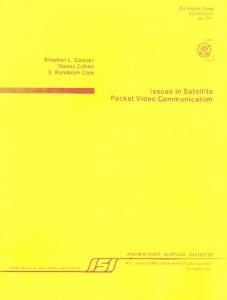
3.5 Complex trace events An instrumentation system may record a single event which must be split into several events to correspond to the graph grammar. For example, a trace event for a multicast or an n-way fork has to be translated into a series of binary forks, and a multiway join or gather has to be translated into a seried of binary joins. If a high-level event includes an activity aspect (some action that takes time) then it should be represented by a separate activity event. By convention, we will place the activity before any and-forks (for a multicast: see Figure 6) or after any and-joins (for a gather). e1
e2
e3
e4
Object A f f
Object B1
e9
Object B2
e10
f e7
e8
Object Bn e5
e6
Figure 4: Example of a Multi-cast Communication
3.6 Discussion In summary, the service-structured computation model assumes scenario causality, linear time, and non-interleaving of actions. Scenario causality associates events with a process and with objects, and segments each object's behavior into individual periods of service. Linear-time allows scenario event graphs to be derived from execution traces. The non-interleaving properly characterizes concurrency within a scenario and it captures the object architecture. In addition: • An object only executes on behalf of a process (i.e., all execution has a cause).
Page 14
• For a process to proceed it needs an object to execute on its behalf (i.e., no unobservable execution). • A scenario by assumption always completes (i.e., it does not deadlock). • An object cannot atomically accept a message and send a message in the same event (i.e., observations are unambiguous). • The event instrumentation and monitoring records all events. This is a closed world assumption. This completes the service system definition. It is a good match with many distributed systems and related technologies, such as DCE RPC [Ope92], CORBA[Obj93], Java [LY96, GJS97], and mobile agents [Pra96]. Real-world distributed systems often resemble this class of systems. Server objects respond to RPCs, asynchronous messages, signals, and exceptions. Server objects are shared amongst many simultaneously occurring scenarios. Objects are static or dynamic entities that may exist over the lifetime of many scenarios. Actions take time.
3.7 Scenario Event Graph Axioms The node and edge definitions given above lead to just fifteen ways in which a node can be connected if a SEG (for instance, an “external event” node always has a “start” edge coming from it). These 15 connections are shown in Table 1, and formal proof of their completeness is given in the appendix. The Table includes some object interaction roles which are discussed further below.
4.0 Object Interactions
Considering message exchanges between objects, as in (for instance) [CL94b, CL94a], scenario causality can distinguish at least the following eight kinds of interactions: •
an external message exchange,
•
a blocking RPC [Ope92, BN83],
•
an asynchronous message exchange,
Page 15
•
a deferred RPC (also called an asynchronous RPC),
•
an RPC exception,
•
a multi-cast message exchange,
•
a synchronous bi-directional communication, and
•
a synchronization between software components.
These patterns in turn are a useful part of re-engineering for understanding the application.
4.1 Characterizing Message Exchange Protocols in a Scenario Event Graph Characterizing a message exchange protocol requires using information from both the process event graph and the object event graph parts of a scenario event graph. In Figure 3, consider the remote procedure call made from the Client Object to the Middle Object. The subgraph {e3, e4, e8, e12} of Figure 3 corresponds to a pattern for a blocking RPC, with the properties: • the process subgraph aspect is linear, • the beginning and end are in one object, with no nodes between them in the object subgraph aspect • The middle is associated with other objects Note that the RPC could not be identified when the two subgraph types were examined separately.
e3
e4
Client Object e8
Middle Object
e9
e10
e1
e12
p
p
Figure 5: Object Execution Graph of an RPC Message Exchange
e3
e8
e9
Process P1
e10
e1
e12
&
Figure 6: Process Event Graph of an RPC Message Exchange
Page 16
e4
Figure 3 also has a deferred RPC message exchange which is identified as the sub-graph pattern {e9, e10, e11, e15, e17}. The distinguishing characteristic of the deferred RPC is that the client object can engage in actions (e10) between the initiation of the RPC (e9) and the reception of the reply (e11). This is visible in the object subgraph aspect of the scenario event graph. Events in the scenario event graph take on identifiable roles in message exchange protocols. In Table 1 we can identify: • External request initiation: A request (or exception) was externally generated from outside the system being monitored and it begins a process thread. This is row {A}. • Blocking request initiation: The initiating object cannot proceed until it receives a reply to a request it has just made. This is row {D}. • Non-blocking request initiation: The initiating object sends a message to another object and the initiating object does not block.This is row {H}. • Request acceptance to start a service period: A blocked responding object accepts a new message and begins a new period (rows {E, I, M}). • Synchronization acceptance: A responding object has already began a service period but it is blocked, until it accepts another message. These are rows {J, L, N}. • Sending a reply to a blocking request: A replying object sends a reply to the blocked initiating object. These are rows {F, H}. • Acceptance of a reply: A blocked initiating object receives the reply to its blocking request. These are rows {G, K}. During the execution of a message exchange protocol element, an object will act out a role in the message exchange protocol. The different message exchange protocol roles are discusses next.
Page 17
Node Connection Interpretation (A) External system request.
Allowed Protocol Role(s)
Node Connection Figure
No object
E st
(B) End of the object period and process thread.
Any role
p (C) A process action event.
Any role
(D) Initiation of an RPC message exchange.
Initiator or Forwarder
(E) Acceptance of a message sent using an RPC message exchange.
Responder or Forwarder or Replier
(F) Sending the reply to an RPC message exchange. The responding object’s service period ends.
Replier
(G) A blocked initiating object in an RPC message exchange receives the reply. The replying object ended its service period after it sent the reply.
Initiator
p p
An and-join node is not used because there is only one process thread. (H) There are three possible interpretations of this node connection axiom: (1) An initiating object initiates an asynchronous message exchange. (2) A replier object sends the reply to an RPC message exchange and it does not end it service period but continues executing. (3) A forwarding object forwards the message to another responding object. (I) A blocked object that is not executing in a service period now accepts a message that was sent asynchronously.
(1) Initiator or (2) Replier or
f
(3) Forwarder Responder or
f
Forwarder or Replier
p (J) A blocked object that is executing in a service period completes a synchronization by accepting a message. The message was sent using an RPC message exchange.
Responder or Forwarder or Replier
Table 1: Scenario Event Graph Node Connection Axioms
Page 18
&
Allowed Protocol Role(s)
Node Connection Interpretation (K) A blocked initiating object in an RPC message exchange receives the reply to its message. The replying object did not end its service period after it sent the reply.
Initiator
(L) A blocked object that is executing in a service period completes a synchronization by accepting a message. The message was sent as an asynchronous message exchange.
Responder or
(M) A blocked object that is not executing in a service period now begins executing because of an external request.
Initiator
Node Connection Figure
f
& f
Forwarder or Replier
& st p
(N) A blocked object that is executing in a service period completes a synchronization by accepting an external request.
(O) An RPC exception condition which unblocks the initiating object in
Responder or Forwarder or Replier
st
&
Initiator
st
an RPC message exchange.
& Table 1: Scenario Event Graph Node Connection Axioms
4.2 Roles of Objects in Message Exchange Protocols Scenario causality takes advantage of the observation that, from an application viewpoint, when an object is involved in a message exchange, its future execution is restricted so that it does not violate the semantics of the message exchange protocol. These restrictions are identified by the protocol role an object plays in the message exchange protocol. The role is important because it limits the future events (i.e., scenario event graph nodes) the object may record. For example, a client object that initiates an RPC cannot execute until it receives a reply or an exception. By inspection, the four types of message exchange protocol roles are: • An initiating object sends messages to request services from other objects. • A responding object accepts a message from an initiating object and provides a service.
Page 19
• A forwarding object accepts a message, executes, and then forwards the message to another object for further processing. • A replier object sends a reply to an initiating object to indicate the initiating object’s request has been completed and the initiator can continue. The object roles that are identified for each node connection axiom and the corresponding interpretation are given in the middle column in Table 1.
4.3 Examples of Interactions To clarify the semantics of the scenario event graph and the message exchange protocol role types, example scenario event sub-graphs are presented for: an asynchronous RPC, object synchronization, bidirectional synchronous communication, the RPC exception, and the forwarding message exchange. The scenario event graph figures follow these conventions: time proceeds from left to right, the consecutive nodes of an object are at the same vertical level, and the consecutive nodes of a process thread can crossover to different objects (e.g., blocking RPC). Prior examples of the RPC, asynchronous, and deferred RPC are given in Figure 3. A multi-cast message exchange was shown in Figure 4. 4.3.1 Asynchronous RPC An asynchronous RPC is an RPC message exchange protocol that is constructed from asynchronous messages and this is shown in Figure 7. It is a paired set of asynchronous messages with the first one being the initiating RPC message and the second being the reply. It is deduced that this is an RPC because the initiating object (Object A) does not record further events so it is assumed to be blocked until it receive the reply message from Object B. In this example, Object B continues executing once the reply message is sent to Object A. This deduction relies on the closed world assumption. 4.3.2 Synchronization A synchronization occurs when the synchronizing object has started a service period and it must accept another message to continue execution. There are four possible ways a
Page 20
synchronization occurs. The first case is where the message was sent using a blocking protocol (Figure 8). The second case is where the initiating object uses an asynchronous protocol to send the message (Figure 9). The third case occurs where a blocked initiating object receives its reply to a message that used an RPC protocol (Figure 10). This third case is characterized as a new process thread being forked for the reply. The last synchronization case involves an external event being accepted (Figure 11). Figure 12 is an example of a bidirectional synchronous communication where two objects exchange messages by sending and receiving messages simultaneously. In this example, the andfork node represents the sending of the message, the and-join node represents the reception of the message, and the action nodes represent the duration of the message exchange. Note that the andfork event, and-join event sequence are interpreted as happening simultaneously even though an order is implied by the graph. 4.3.3 Forwarding A forwarding message exchange occurs when the initiating object blocks on its message request and the first responding object asynchronously sends the message to another responding object [HWRI99]. Each responding object can continue to forward the message to other responding objects. The last responding object in the series sends a reply directly to the blocked initiating object. This type of message exchange protocol occurs when an object acts as a request dispatcher [Gen81] or as a form of rate control for an object pipeline. An example forwarding message exchange is shown in Figure 13, where: the initiating object (Object A) sends the message and blocks, the first forwarding object (Object B) handles the message, and forwards it in an asynchronous fashion to another forwarding object (Object C), Object C handles the message further and forwards it to Object D which replies to the initiating object. 4.3.4 RPC Exception An RPC exception occurs when an object that initiated an RPC becomes unblocked due to an exception and not a reply. An exception condition may result from a time-out condition, a signal
Page 21
Object A
&
f
f
Object B Figure 7: An RPC Message Exchange using Asynchronous Communication
Object A Object B
&
Figure 8: A Responder Object Synchronization from an RPC Message Exchange
Object A f Object B
&
Figure 9: A Responder Object Synchronization from an Asynchronous Message Exchange
&
Object A f Object B
Figure 10: An Initiating Object Synchronization from an RPC Message Exchange
E
st Object A
&
Figure 11: An Object Synchronization from an External message
Page 22
Simultaneous Object A
&
f f Object B
&
Figure 12: An Example of Bidirectional Synchronous Communication
Object A
&
Object B f
f
Object C f Object D Figure 13: A Forwarding Message Exchange with Two Levels of Forwarding
Object A
&
Object B
&
f
f
Object C f Object D Figure 14: A Forwarding Message Exchange with Blocking Communication
Page 23
from the environment, or a high-priority message interrupting the initiating object. Two example characterizations of an RPC exception are shown. The first type of RPC exception (Figure 15) is the result of an external event such as a software interrupt, so the initiating object resumes execution before receiving the reply to its initial message. The second type of RPC exception occurs when a blocked initiating object accepts a message in place of a reply but the message is not causally connected to its initial message. Figure 16 is an example of this situation. In this example, initiating Object A receives a message from Object C that is interpreted as a reply, but Object C has no causal connection to the RPC. E
st &
Object A Object B
Figure 15: An RPC Exception from an External Event
E
st Object C f Object A
&
Object B Figure 16: An RPC Exception from a Causally Unconnected Event
4.3.5 Message Exchange Roles: Summary The possible message exchange protocol roles associated with each message exchange are listed in Table 2. The reader will notice that what initially seems to be a responding object may later become a forwarding or replier object due to its behavior after receiving a message. The
Page 24
asynchronous message exchange has only two protocol roles: the initiator and the responder. A multi-cast message exchange is similar because a multi-cast is analogous to a series of asynchronous message exchanges. An RPC, deferred RPC, or asynchronous RPC message exchange has two roles: an initiator and the responding object that later becomes a replier object. Message Exchange Type
Initiator Role Responder Role Replier Role Forwarder Role
Asynchronous, Multi-cast
Yes
Yes
No
No
RPC, Deferred, RCP, Asynchronous RPC
Yes
No
Yes
No
Bi-directional synchronous
Yes
Yes
No
No
Forwarding
Yes
No
Yes
Yes
External
No
Yes
No
No
Table 2: Protocol Roles that Occur In a bi-directional synchronous communication message exchange, both objects begin as initiating objects and then become responding objects to receive the sent message. A forwarding message exchange (Figure 13) has three roles: the initiating object (Object A) blocks after sending its message. The first forwarding object (Object B) receives the message from the initiating object, executes and then forwards it to another object (Object C). Object C receives the message, executes, and then forwards it again. The last object in the forwarding chain performs the role of a replier, sending the reply message back to the blocked client. The last message exchange listed in the table is the externally initiated message exchange. In this case there is no initiating object because the source of the message is outside of the system. However, there is a responding object which receives the external message. An example of a responding object is Object A in Figure 11.
4.4 More Message Exchange Protocol Variations The message exchange protocols that have been presented can vary in several fashions. First, all of the RPC message exchanges could be constructed using asynchronous messaging, just like in Figure 7. Secondly, the forwarding of a message may use internal blocking or asynchronous message exchanges. Third, in any of the instances, a responding object may accept a message that
Page 25
forms a synchronization. Lastly, a variation of a forwarding message exchange occurs when the message is forwarded using an RPC protocol (Figure 14). It should also be emphasized that server objects can be involved in other message exchanges while executing, looking like client objects to lower layers of servers.
5.0 Comparing Scenario Causality with Potential Causality STUFF TO FIND A HOME FOR OR REMOVE The most widely used event ordering relation is called “potential causality” because it orders the events temporally [Lam78, SM94]. Potential causality is the smallest transitive relation that orders: • the succeeding events in an object, and • the send and receive communication events between objects so that a send event always precedes its corresponding receive event. Potential causality answers questions such as, “Did event e 1 happen before event e 2 in the distributed system?” Thus, potential causality has also been called the happened before relation. Potential causality is represented as a partial order where it is assumed that if two events cannot be ordered then the events may have occurred concurrently. This partial order topology of potential causality can be expressed as a graph grammar with one node type (an untyped event) and one edge type that identifies the succeeding node for a given node. Potential causality generates a global event graph which orders all of the potentially causal (i.e., predecessor) events and the (potentially) concurrent events are on parallel branches of the graph. Scenario causality includes only those ordering relationships that are certain to be valid within a scenario. It is more expressive because it has several edge types to represent different types of causal relationships. Scenario causality is described as: “an event e 1 is a scenario cause of event e 2 if there is a sequence of events from event e 1 to event e 2 in the same scenario.”
Page 26
Scenario causality characterizes several application level communication protocols (or message exchange protocols) that potential causality cannot characterize. A clarification is needed about the definition of scenario causality. If event e 1 : v 1 = { x ← y } which precedes the event e 2 : v2 = { a ← b }
in the same scenario, then event e 1 is considered to be a scenario cause of event e 2 ,
even though there is no direct dependency between the variables v 1 and v 2 . There are two reasons for this position. First, the developer ordered those two statements so there is an inferred causal dependency which may later manifest itself. Second, and more practically, the actual ordering of the program statements ensures that event e 2 could not execute without event e 1 first occurring in that scenario. The next section examines the scenario event graph’s semantics. The scenario event graph figures will no longer show the icon for the object action node because it is the default node type for the object event graph.
6.0 A Class of Logical Clocks The topology defined so far gives the requirements for a metrication and a complete clock. these requirements can be summarized as: ???? anything new... or do we refer to items before Any generic properties of this class, beyond the angio trace example? The feasibility of creating a complete clock definition has been demonstrated by creating a logical clock specially for building performance models of software. Include the following two sections, or some of it. Generic description. refer to proprietary version at the end.
7.0 An Overview of Automated Model Construction Scenario causality is the basis for a Model Making Automation Process (MMAP) which is a technique for the (automated) construction of scenario models [Hri98a]. MMAP is based on the
Page 27
novel concept of using several graph grammars to convert execution traces into abstract scenario models. Using a graph grammar formalism allows the scenario models to be constructed and analyzed in an automated fashion. MMAP, which is a generalization of a process for the automated construction of a performance model of distributed applications [HWRI99, Hri98b], is briefly described here to illustrate how scenario causality and the scenario event graph can be used for software engineering purposes. MMAP is a chain of formal transformations. At each step in the chain it converts an input model into a more abstract or domain specific model. MMAP's general strategy for transforming a model from its input domain to its target domain is as follows. First the application specific domain language of the input model domain and the target domain are both described as separate graph grammars. Then a graph transformation from the application specific language of the input domain (the input graph grammar) to the application specific language of the target domain (the target graph grammar) is developed using graph rewriting rules to define semantic equivalences of sub-graphs in the input and output domains. The several model domains of MMAP are identified in Figure 17. They are listed in the order in which data flows to construct a model: (a) Program language statement: the object’s source code statements. (b) ANGIOTRACE instrumentation: Embedded instrumentation that atomically generates and records ANGIOTRACE events when language statements are executed. (c) ANGIOTRACE event records: The recorded events which can be ordered in accordance with scenario causality using special logical timestamp values. (d) Scenario event graph: A graph grammar that characterizes all possible scenarios. It is the topic of this paper. (e) Scenario model: A model type that characterizes the execution of a scenario for further analysis. This includes the involved objects, their individual actions, the messages, and the message exchange protocol elements.
Page 28
(f) Domain specific model: A view of the execution, that may have additional information included, for domain analysis purposes. The algorithmic graph grammar formalism is used as the basis for the model transformation machinery which is implemented by the PROgrammed Graph REwriting System language and its corresponding toolset [Nag87, Ehr87, Sch90, Sch91b, Sch91a, SWZ95, Sch97]. (a) Program language statement
#1) System execution (b) Angiotrace instrumentation
#2) Instrumentation execution (c) Angiotrace events #3) Event ordering (d) Scenario event graph #4) Scenario event graph (SEG) analysis (e) Scenario model #5) Domain model construction
Additional domain information
(f) Deployment diagram
(f) Sequence diagram
(f) Performance model
Figure 17: MMAP Data Flow
Formal transformation
For illustrative purposes, there are three domain specific models identified in Figure 17 that MMAP can construct. It should be apparent that the event traces of Figure 3 can be used to reconstruct the sequence diagram of Figure 2. If information about the deployment of the software is added, then a deployment diagram can be produced. It is described in [HWRI99, Hri98b] how a
Page 29
performance model can be constructed from several scenario models. MMAP may also generate other types of models.
8.0 Implementing the SEG as a Logical Clock The two steps in Figure 17 which move from the program language statement to a scenario event graph are linked by a new type of logical clock called an ANGIOTRACE.1 The ANGIOTRACE is the metrication for the scenario event graph topology. This section provides an informal discussion of how the
ANGIOTRACE
events can form a scenario event graph, providing insight into the
development of the logical clock metrication and implementation. When referring to an angiotrace the term event will be used in place of the term node. The name
ANGIOTRACE
is derived by analogy from an angiogram. An angiogram is a
visualization of an individual's blood flow that is produced by injecting a radio-opaque dye into the blood stream and taking an X ray of the dye dispersion. Similarly, an ANGIOTRACE assigns a different software dye to each scenario so that each scenario's event records can be distinguished and ordered. The software dye consists of an object timestamp to construct the object event graph and a process timestamp to construct the process event graph. The underlying formalism of the angiotrace is that of partial order multi-sets [Pra86] because it has more than one timestamp and more than one type of edge. Instead of a single event ordering relation, an ANGIOTRACE uses a set of partial ordering relations to construct the scenario event graph. There are six event ordering relations for identifying the causal relationships that exist between a given event’s succeeding or preceding event(s). These relations are used to construct a scenario event graph because each ordering relations will add a specific edge type between two nodes when it is satisfied; (if an ordering relation cannot be satisfied then an edge is not added. The ordering relations that are provided are:
1. It should be noted that a form of ANGIOTRACE was described in [HRW95, HWRI99] but the ANGIOTRACE instrumentation that is compatible with scenario event graph is described in [Hri98b].
Page 30
• Find the succeeding node in the object event graph and add an object’s next period edge if the succeeding node is a period start node, otherwise add a next object edge. • Find the succeeding node in the same process thread and the same object event graph and add a next process edge between the two nodes. • Find a succeeding process event graph node that is not in the same object event graph and add a start the process edge if the source event is an external node, otherwise add a process thread’s fork edge. The three remaining ordering relations are used to find the preceding node given its successor event. Like most other logical clocks, the angiotrace timestamps are counter values with prescribed rules for incrementing the counters to guarantee uniqueness and event ordering. The rules for incrementing the counters and ordering the events using the timestamps must be able to identify and reconstruct each possible ordering relationship in Table 4. If the metrication satisfies this requirement then it will be able to characterize all possible executions of the distributed system since these are the only valid events orderings.
9.0 Conclusions Scenario causality has been defined here for the purpose of identifying and order the events that are recorded for a scenario, recovering important contextual information that cannot be retrieved using conventional means. There are several new applications that should be able to make use of scenario causality. For example, the ability to identify a type of scenario would enable the provision and enforcement of a quality of service for a type of scenario. Identification of a scenario could allow for more efficient approaches to checkpointing for roll back [PK93] or the detection of consistent cuts [CB89] because unimportant scenarios types could be ignored. The scenario information is useful for understanding applications with persistent objects that can remain dormant because, in this situation, wall clock time cannot be used to establish any causal links between events.
Page 31
A new, event based reference model of distributed system execution was developed called the scenario system event model. A novel aspect of the scenario system event model is that it uses the process and the object views in a distributed system to construct the scenario and global, system level view. A graph type is defined for each of these views. The scenario system event model defines the minimum information needed to reverse engineer scenarios. In particular, it specifies that the start and end of a process, as well as the start and end of object service periods must be characterized. This is in addition to the local actions and communication actions of the objects. The logical clock topology defined for scenario causality is a graph grammar with events that are represented as typed nodes and different types of causal relationships are captured as typed edges. A scenario event graph is formed using this graph grammar. The family of valid graphs that can be constructed are defined by the node connection axioms of Table 1 and the node connectability table (Table 4). Together, these two tables defines the topology of a logical clock that is consistent with scenario causality and they serves as the specification for a logical clock implementation. The definition of scenario causality presented here is a for message passing distributed system. Scenario causality characterizes more application level, message exchange protocols than conventional techniques. The message exchange protocols that are characterized are: an external message exchange, a blocking RPC, an asynchronous message exchange, a deferred RPC (also called an asynchronous RPC), an RPC exception, a multi-cast message exchange, a synchronous bi-directional communication, and a synchronization between software components. The results can be also applied to software systems which are a sub-set of a message passing system (e.g., a single threaded object-oriented application or a parallel message passing application). In principle, scenario causality should be extensible so that it can characterize additional application specific message exchange protocols, such as replication [Bir87], atomic transactions [Lis88], object migration [SHK92], or tuple spaces [ACG86, CG89]. Extensions to characterize scenario causality for non-message based exchanges between objects may also be possible (.e.g, semaphore, condition variable, synchronization barriers). The development of an extension would
Page 32
follow the methodology outlined in section 2.0, modifying or adding to the scenario system event model, the node connection axioms of Table 1, and the node connectability table of Table 4. Using a graph grammar to define scenario causality enables graph grammar community to participate in the analysis of scenarios [Sch90, Nag79]. For example, sophisticated tools for programming with graph languages (e.g., PROGRES [SWZ95, Nag96]) can be used for system analysis. In particular, the use of a graph grammar has allowed different types of models to be automatically generated from a scenario event graph model [Hri98a]. The results of this research can be applied to give sharper results in areas that have been studied previously with potential causality: distributed algorithm implementation [Mor85], system feature implementation (e.g. causal memory [AHJ91], causal message ordering [BSS91]), design recovery [KB95], global state recording [CL85, FZ90, Mat93, SK86], global predicate evaluation [CM91, HW88, HK90], trace replay [NM92, LM87], design recovery [KB95], describing event patterns [LKA+95, Fid91], the visualization of system execution [KB95], automatically constructing software performance models [HRW95, HWRI99], and race detection [HMW93]. A novel aspect of this work is that it is the first time that a logical clock’s topology has been directly addressed as an attribute. A significant result from this is the idea that there is more than one form of cause-and-effect relationships which can be characterized and exploited in analysis. In support of this four types of causality are listed that have been identified in the logical clock literature: • Real causality is the event ordering that is consistent with both the purpose of the software and a particular execution of that software. Recovering real causality is impossible in practice because it necessitates full knowledge of each: object’s behavior, the variables’ initial values, the processes, and the execution environment. • Imposed causality is an ordering between timestamps imposed by an algorithm and this ordering does not have to correspond to the event order during execution. An example is the ordering produced by the scalar logical clock [Lam78]. • Potential causality has been used to provide a temporal ordering. An example is the event ordering produced by vector logical clocks [Fid91, Mat88].
Page 33
• Scenario causality has been introduced here to enable the reverse engineering of scenarios. The natural progression is to continue to define other application or domain specific forms of causality. Potential causality can be reconstructed from scenario causality, by replacing next period edges by causal edges and using the global event graph.
10.0 Acknowledgments This research was supported by the Natural Sciences and Engineering Research Council (NSERC), by Bell Canada, Nortel, and DY-4, through an industrial research chair.
11.0 Appendix: Proof that Scenario Causality is Complete and Consistent This section proves by enumeration that the node connection axioms of Table 1 are the only valid ways to connect nodes and characterize scenario causality. First a general representation of a scenario event graph node and edge is identified. Next, all of the ways in which a scenario event graph node can be connected to its preceding and succeeding node are enumerated. Finally, those node connection axioms whose causal interpretation is not consistent with scenario causality are eliminated. The result of the proof is a node connectability table that determines all of the valid ways each node connection axiom can connect with all other node connection axioms, thereby characterizing all valid scenario event graph’s.
11.1 Characterizing Scenario Causality between Any Two Nodes In the scenario event graph a node is a six-port building block (Figure 18), where a port is the source or target of a single edge. The position of a port identifies the valid edge type that can connect with it, as well as the direction of the edge. There are six ports because a scenario event
Page 34
graph node has at most three incoming and three outgoing edges since it is the super-position of a binary graph (i.e., the process event graph) and a linear graph (i.e., the object event graph). The six port types are: • InObject: the target of an edge connected to the preceding node in the same object event graph. • InProc: the target of an edge connected to the preceding node in the same process thread and in the same object event graph. • InProcExt: the target of an edge connected to the preceding node that is part of the same process event graph but not in the same object event graph. When an external event occurs or a message is received by an object this port is the target of an edge. • OutObject: the source of an edge connected to the succeeding node in the same object event graph. • OutOp: the source of an edge connected to the succeeding node that is in the same process thread and in the same object event graph. • OutOpExt: the source of an edge connected to a succeeding node that is part of the same process event graph but in another object event graph. This port is the source of an edge when an external event occurs or a message is sent by an object. For this portion of the proof the type of an edge is not important. An edge’s type identifies the type of scenario causality between two nodes, but the proof only needs to identify that a scenario causal relation (an edge) exists. Based on this six-port building block model, consider all the combinations of ways in which these ports may (or may not) have edges attached to them. For each port, assign a binary value 1 if it has an edge attached or a 0 if not. A binary number, called the node connection value in Table 3, can be constructed where the bit positions are, from most significant bit to least significant bit:
InProc, InObject, InProcExt, OutOp, OutObject, OutOpExt
Page 35
And-fork edge Next process edge Start SEG edge Next process edge
InProc
InProcExt
OutOp
InObject
OutOpExt
OutObject
Next object edge Next object period
Next process edge
Next object edge Next object period
And-fork edge Next process edge Start SEG edge
Figure 18: A Scenario Event Graph Node as a Six-Port Device
This means there are 64 possible values. However, many of these connections are invalid because they violate the causal interpretation of the process event graph, the object event graphs, and the scenario event graph. The constraints due to scenario causality fall into three categories: • Structural constraints: each node and edge type is unique, having a specific interpretation that allows (or prevents) it from connecting to other node types. • Consistency constraints: scenario causality characterized by the object event graph and the process event graph must be consistent. • Interpretation constraints: the scenario event graph must be unambiguous in its characterization of causality. Each constraint type and its effect on the possible node connection axioms are considered next. The structural constraints ensure each node has unique properties. The thread end node is the only node type to finish a process thread. The thread begin node is the only node type that is allowed to begin a process thread. The external node has no cause. The and-join node has two causes from different process threads. The and-fork node is the cause of events in two process threads. The process action node represents a local action of an object that can have duration. The period start node identifies the beginning of an object’s service period.
Page 36
The following consistency constraints ensure that the scenario event graphs have a consistent causal interpretation: • For a scenario to proceed it needs an object to execute on its behalf. • An object only executes on behalf of a scenario. • A scenario always successfully completes (i.e., it does not deadlock). There are two results that follow from these constraints: a node cannot be the source of a next object edge without also being the source of a next process edge, and a node cannot be the target of a next object edge without also being the source of a next process edge. Note that a node can be the source of a next process edge without being the source of a next object edge because the scenario can continue in another object (i.e., RPC reply). There are two interpretation constraints that need to be considered. The first constraint is that an object can either accept a message or send a message but it cannot do both for the same node. Otherwise the causal ordering is ambiguous because it is not known which action, sending or receiving, occurs first. The second constraint is that objects do not interleave their service periods. The set of valid node connection axioms can then be found by enumerating the possible node and edge connections and then removing the invalid possibilities. This is summarized in Table 3 and expanded in Table 5 of Appendix A. For example, an external node will only be the source of a start the process edge on the OutOpExt port so it has a hexadecimal node connection value of 01. The thread begin node is the target of a start the process edge on the InProcExt port and it sources a next process edge and a next object edge in the same process thread (i.e., OutOp and OutObject ports). The thread begin node then has the hexadecimal node connection value of 0E. Several example invalid node connections arise from the interpretation constraint preventing a node from receiving and sending a message, which translates to the node being the target of an edge on the InProcExt port and a sources of an edge on the OutOpExt port. As shown in Table 3 this eliminates several node connection values, such as 09, 0B, etc. The node and edge typing is added to distinguish the cases where a single node connection value in Table 3 can give rise to several node connection axioms in Table 1 which are distinguished
Page 37
Valid Node Invalidated Node Connection Connection Values Value (hex) (hex)
Explanation
Nodes with no edges are not allowed because a process thread must have at least two nodes: a begin node and an end node. Only an external node is allowed to have an effect without a cause. This is item 01 {A} in Table 1. A node cannot both receive a message and send a message.
The scenario is stopped if there is not an outgoing object edge without an outgoing process edge. A next process edge output in the same object period (OutOp) must have a corresponding next object output edge (OutObject), otherwise the object is deadlocked. The receiving object is blocked (no InObject edge) and it becomes unblocked by accepting a message (InProcExt). These are items {E, I, M} in Table 1. A node must have a next process edge as an input, either InProc or InProcExt, to proceed to the next node, otherwise the object executes without a scenario which is not allowed in a scenario system event model. The object is blocked (i.e., not InProc), becoming unblocked by accepting a message on InProcExt, continuing execution of the scenario by sourcing edges on OutOp and OutObject. This is items {G, K, O} in Table 1. A node must have an object input edge if it has a process input edge in the same object period. The thread end node is the only node type that is allowed to terminate the scenario event graphs. This is item {B} in Table 1. Sending of the reply to an initiating object in an RPC message exchange and the replying object finishes its service period. This is item {F} in Table 1. Initiation of an RPC message exchange. This is item {D} in Table 1. A node cannot have an output process edge in the same object (OutOp) without a corresponding object output edge (OutObject) because a scenario cannot progress in the same object without the object progressing. The scenario continues in the same object. This is item {C} in Table 1. A process thread is forked. This is item {H} in Table 1. A message reception is accepted and the accepting object was already processing a message (InObject). This is characterized by items {J, L, N} in Table 1.
02, 03, 04, 05, 06, 07 09, 0B, 0D, 0E, 17, 19, 1B, 1D, 1F, 29, 2B, 2D, 2F, 39, 3B, 3D, 3F 0A, 1A, 32, 3A 0C, 14, 1C, 24, 2C, 34, 3C
0E 11, 12, 13, 15, 16
1E
30
21, 22, 23, 24, 25, 26, 2A, 2E 08, 10, 18, 20, 28, 38
31 33 35
36 37 3E
Table 3: Enumeration of the Possible Node Connections
Page 38
0
by the node and edge types. Those sets of nodes which are differentiated by the type information are: {J, L, N}, {K, G, O}, and {E, M, I}.
11.2 Determining Node Connectability This sub-section identifies all valid causal relationships between any two events (i.e., scenario event graph nodes), proving that the node connection axioms characterize all valid scenarios. This proof of completeness is by enumeration. The connectability table (Table 4) identifies how two nodes may be connected based on the port definition and edge type information. It is constructed by identifying all of the valid predecessor and successor node connection axioms for each node connection axiom of Table 1. This is done by inspection: for each node connection axiom in Table 1, the set of possible predecessor and successor node connection axioms are identified by matching the outgoing and incoming edge types. However, this set must be pruned by removing the node connection axioms which are not consistent with the message exchange role or where the scenario causality interpretation is invalid. There are two invalid node connections which have been removed from the Table 4. They are: • Node connection axiom D cannot source a next process edge from port OutOpExt to the target InProcExt of a node connection axiom G. The justification is that an RPC initiation (D) should not be a reply message that unblocks another initiating object already in an RPC message exchange (G). • Node connection axiom F cannot source a next process edge from port OutOpExt to the target port InProcExt of a target node connection axiom E or J. The justification is that an RPC reply (F) should not be considered to be the initiation of another RPC message exchange (E or J). The usefulness of a proof by enumeration was made evident when, to the author’s surprise, these invalid node connections were found.
Page 39
Node Conne Node Type ction Axiom
Previous Node Connection Axiom in the Same Object Event Graph (InProc and InObject)
Previous Node Successor Node Connection Successor Node Connection Axiom in a Connection Axiom Axiom in a Different in the Same Object Different Object Event Event Graph Object Event (OutOp and OutObject) Graph Graph (OutOpExt) (InProcExt)
A
External
n/a
n/a
n/a
M, N, O
B
Thread end
C, E, G, H, I, J, K, L, M, N, O
n/a
E, I, M
n/a
C
Action
C, E, G, H, I, J, K, L, M, N, O
n/a
B, C, D, F, H, J, L, N n/a
D
Action
C, E, G, H, I, J, K, L, M, N, O
n/a
G, K, O
E
Action
B, F
D
B, C, D, F, H, J, L, N n/a
F
Action
C, E, G, H, I, J, K, L, M, N, O
n/a
E, I, M
G
Action
D
F
B, C, D, F, H, J, L, N n/a
H
Fork
C, E, G, H, I, J, K, L, M, N, O
n/a
B, C, D, F, H, J, L, N I, K, L
I
Thread begin
B, F
H
B, C, D, F, H, J, L, N n/a
J
And-join
C, E, G, H, I, J, K, L, M, N, O
D
B, C, D, F, H, J, L, N n/a
K
And-join
D
H
B, C, D, F, H, J, L, N n/a
L
And-join
C, E, G, H, I, J, K, L, M, N, O
H
B, C, D, F, H, J, L, N n/a
M
Thread begin
B, F
A
B, C, D, F, H, J, L, N n/a
N
And-join
C, E, G, H, I, J, K, L, M, N, O
A
B, C, D, F, H, J, L, N n/a
O
And-join
D
A
B, C, D, F, H, J, L, N n/a
Table 4: Node Connectability Table
Page 40
E, J G