Page 1 of 10
IET Radar, Sonar & Navigation This article has been accepted for publication in a future issue of this journal, but has not been fully edited. Content may change prior to final publication in an issue of the journal. To cite the paper please use the doi provided on the Digital Library page.
Practical classification of different moving targets using automotive radar and deep neural networks Aleksandar Angelov1, Andrew Robertson2, Roderick Murray-Smith3, Francesco Fioranelli1* 1
School of Engineering, University of Glasgow, Glasgow, UK NXP Semiconductors, Glasgow, UK 3 School of Computing Science, University of Glasgow, Glasgow, UK *
[email protected] 2
In this work, we present results for classification of different classes of targets (car, single and multiple people, bicycle) using automotive radar data and different neural networks. A fast implementation of radar algorithms for detection, tracking, and micro-Doppler extraction is proposed in conjunction with the automotive radar transceiver TEF810X and microcontroller unit SR32R274 manufactured by NXP Semiconductors. Three different types of neural networks are considered, namely a classic convolutional network, a residual network, and a combination of convolutional and recurrent network, for different classification problems across the 4 classes of targets recorded. Considerable accuracy (close to 100% in some cases) and low latency of the radar pre-processing prior to classification (approximately 0.55s to produce a 0.5s long spectrogram) are demonstrated in this paper, and possible shortcomings and outstanding issues are discussed. 1. Introduction
Autonomous vehicles have been gaining significant interest in the past few years, with considerable attention and investments from technology-intensive companies (such as data management and algorithms developers, vehicles and electronic sensors and systems manufacturers), governments and academic research community, and media and the general public [1-3]. As research in this vast field grows, an attempt of standardising the different levels of autonomy that ADAS (Advanced Driver Assistance Systems) can enable in ground vehicles has been made, specifying six levels ranging from 0 to 5, from rather standard car accessories such as ABS (Antilock Braking System), to fully autonomous dynamic driving with little to no inputs from the human driver [2]. To achieve complete driving autonomy, the capability of sensing the surrounding environment and other moving entities, other vehicles or humans and animals, is paramount. Different sensing technologies have been proposed [4]. Cameras are suited for objects classification exploiting colour and texture data, and can be relatively cheap compared to the other types of sensors, but may suffer from limited depth of view and adverse weather and light conditions, as well as requiring high data processing power, depending on the image classification algorithm. LiDAR uses rotating laser arrays to generate an accurate 3D map of the surrounding environment around the autonomous vehicle, but this type of sensors are still rather expensive and may require significant computational power to address the adverse effect of light and weather (rainy, foggy, snowy conditions). Radar sensors provide the advantage of not being affected by light and weather conditions, as well as exploiting mature range-Doppler and classification processing developed for different end applications over the years [5]. However, the applicability and adaptation of these techniques to the specific automotive context, and the development of the most suitable processing to fuse information from different radar channels and heterogeneous sensors are still open research
questions. In particular, significant research in the context of automotive radar has been devoted to the issue of detecting and classifying accurately vulnerable road users, such as pedestrians, to preserve their safety. One of the earliest classification studies on automotive radar reported over 90% accuracy when distinguishing vehicles and pedestrians [6], as well as other objects [7], by extracting features from micro-Doppler signatures combined with Joint Probability Data Association tracking, in order to account for discrepancies in amplitude and shape due to aspect angle changes. Although the use of trackers worn by vulnerable road users would help their detection and classification [8], the reliability of the whole system would be poor, as relying uniquely upon compliance of them wearing the devices. Other studies looked at using range-Doppler maps as the domain to perform classification. Object tracking through clustering algorithms and a linear classifier were used to distinguish vehicles and scenarios of walking pedestrians in [9], and in [10] features related to the size, orientation, and frequency of the pedestrians’ step were used in conjunction with OS-CFAR (Ordered Statistics-Constant False Alarm Rate) and Density Based cluster algorithm. Further works focused on using different domains of information to achieve vehicles-pedestrians classification, such as [11] through the phase characteristics (coherent/non-coherent) of the object signature, and [12] through features related to the differences in Radar Cross Section (RCS) between the different classes of targets, used together with an SVM (Support Vector Machine) classifier. As systems working at higher frequency, tens but also hundreds of GHz, become available, work has been carried out to characterise the radar signatures of pedestrians in the automotive context, such as in [13-15] which considers the frequency ranges around 300 GHz. Another group of studies looked at characterising the radar signatures of cyclists, to highlight differences and similarities with those of pedestrians and vehicles that can be useful to improve their detection and classification [16-18]. Bicycles can travel at significantly higher speed than pedestrians and present high manoeuvrability on the road, as well as at the
IET Review Copy Only
1
IET Radar, Sonar & Navigation
Page 2 of 10
This article has been accepted for publication in a future issue of this journal, but has not been fully edited. Content may change prior to final publication in an issue of the journal. To cite the paper please use the doi provided on the Digital Library page.
same time exhibiting low RCS compared with vehicles; they are therefore a challenging class of targets for automotive radar applications. Many of the classification studies considered some form of “handcrafted” extraction process on the radar data in order to obtain the most suitable combination of features to maximise classification accuracy [19-20]; this often requires significant expertise and inputs from the human radar operator/engineer, thus not lending too well to achieving reliable automatic classification in the large diversity of situations and scenarios expected for automotive radar. To address this issue, an emerging stream of work in the literature has been looking at neural networks as a processing tool to bypass the feature extraction step and enable automatic selection of the most suitable features and meaningful information for classification within the network itself. One of the first work in this aspect was [21], in which Deep Convolutional Neural Networks (DCNN) were given spectrograms directly as input data to distinguish 4 classes of targets (humans, dogs, horses and cars signatures), and 7 different human activities. The DCNN was a scaled-down model of the famous VGG16 (Visual Geometry Group) network that won the ImageNet classification challenge in 2014, and accuracy in the region of 91% was achieved for target identification. Further work on the use of CNNs in the context of human activity recognition for assisted living has been presented [22], focusing on aspects such as most suitable pre-processing and time-frequency distribution for the micro-Doppler signatures [23], combination of information from different radar domains including range-Doppler and range-time to enhance performance [24], different architectures mixing AutoEncoders (AE) with CNNs [25-26], and challenges and strategies to train deep networks effectively with limited experimental radar data available [27]. Other works have looked at classifying different human gaits in the context of area surveillance using ground-based radar, in particular identifying individual pedestrians as opposed to group of multiple people, either using CNNs or Recurrent Neural Networks (RNNs) on the spectrograms [28-29], and at classification of armed/unarmed personnel using multistatic radar [30]. In this work, we present and discuss a modular pipelined approach to achieve near real-time radar data processing and multiple moving object tracking, and to subsequently classify these objects. Three different neural network architectures have been explored – a downscaled version of the network VGG16, utilizing the same block structure; the very deep ResNET-50 [31], which uses shortcuts between network blocks to avoid overfitting and achieve better generalization; and an innovative CNN+LSTM (Long Short-Term Memory) architecture, which is able to extract features from microDoppler spectrogram segments, and learn their representation as time series (sequences of data). This is an innovative approach, as the radar data will be considered by the LSTM network part not as snapshot spectrograms images (as currently done in many works in the literature [22-28]), but as temporal data sequences. Although demonstrated on preliminary results on a small experimental dataset, this classification approach may prove well suited to radar data, exploiting the inherent information from a sequence of radar waveforms, rather than casting the problem as classification of images.
Although the dataset of experimental samples is small, the work presented here aims to demonstrate the potential of this approach. It provides a proof of concept evaluation of lean implementation of radar signal processing necessary for radar micro-Doppler based classification, and of different architectures of neural networks that do not require manual fine-tuning of parameters of external inputs to guide the feature extraction process. These processing steps have been implemented with the following objectives: to use real experimentally-gathered data for training and testing the neural networks, in order to investigate the generalization capabilities of the network architectures beyond the ideal cases of using simulated data. This includes the implementation of radar signal processing for detection and tracking of multiple targets, which can provide good performance even in the presence of significant noise generated within the radar system; to have a significantly low classification latency – below 0.5 seconds, since studies have shown that the average driver reaction time is around 0.7 seconds [33]; to use the micro-Doppler spectrograms directly as input to the classifier and network, avoiding handcrafted features (e.g. Micro-Doppler bandwidth and frequency, Cepstral coefficients, moments of vectors extracted by Singular Value Decomposition, and many others proposed in the literature [20]) - This allows to avoid possible loss of relevant information and fine-tuning of the many parameters involved when defining the feature extraction algorithms. The remainder of this paper is organised as follow. Section 2 describes the experimental setup, the radar kit used, and the data collection protocol. Section 3 introduces the implementation of the radar signal processing developed, and the structure of the neural networks used in this study. Section 4 presents and comments on the experimental results. Finally, section 5 draws conclusions and discusses some possible future work. 2. Experimental setup and data collection All data have been collected using the TEF810X fully integrated automotive radar transceiver manufactured by NXP Semiconductors and S32R274 radar Micro-Controller Unit. The radar operation mode was configured as Frequency Modulated Continuous Wave (FMCW), with linear chirp modulation, and the parameters, shown in Table 1. These parameters were empirically found to provide the clearest micro-Doppler (MD) signatures at visual inspection, as well as providing a reasonable compromise in terms of range resolution, Doppler unambiguous range, and data throughput for fast transferring and processing. The system had 1 transmitter and 4 receiver channels, and digitised data were transferred from the micro-controller unit to a computer via UDP packets. These packets were then decoded to form “frames”, matrices with 512 rows and 256 columns, which essentially correspond to range-time matrices with 256 radar chirp and 256 (after removing FFT mirroring) range bins for each chirp. The time for one frame to be transmitted and received for processing (for all 4 receiver channels) is set internally in the MCU as 50ms, and this is a firmware 2
IET Review Copy Only
Page 3 of 10
IET Radar, Sonar & Navigation This article has been accepted for publication in a future issue of this journal, but has not been fully edited. Content may change prior to final publication in an issue of the journal. To cite the paper please use the doi provided on the Digital Library page.
parameter that cannot be modified in this version of the system. Three different types of movements and targets were recorded, namely a single person walking at an average speed of 4-5km/h (type 1), a car accelerating and decelerating (type 2), a bicyclist following the trajectory of an eight figure (type 3), and finally two people walking side by side (type 4). All activity types were performed with objects moving towards and away from the radar covering a distance of around 0-17 metres, at 0 degree aspect angle (radial trajectory with respect to the line-of-sight of the radar), with some little variability for the bicyclist to turn when cycling towards and away from the radar. The radar was positioned approximately 0.7 metres above the ground, to correspond to the height at which automotive radar is usually mounted on a car. This also allows to capture the micro-motions contributing most to the MD effect, such as hands, torso and the upper leg parts from walking people; the body of a moving vehicle; and bicycle frame/pedalling legs. Around 30 minutes of data each were collected for the single person walking and the car, and approximately 15 minutes each for the bicycle and the multiple people class. The raw digitised data were then divided in blocks, which are the starting point of the processing steps described in the next section. Number of samples per chirp
512
Number of chirps per frame
256
Chirp bandwidth
1.0 GHz
Chirp duration
25.6 μs
Carrier frequency
76.5 GHz
ADC Sampling Frequency
20 MHz
TX/RX channels
1/4
Radar field of view (azimuth and elevation)
±35° at 50m / 7.5°
Table 1: Radar parameters for the data analysed in this paper 3. Data processing and neural networks architecture As described in section 1, a lot of research has been conducted on target classification using the MD signature of objects. When the target signature is spread across many different range bins, the different target contributions need to be aggregated prior to performing STFT (Short Time Fourier Transform), or an alternative time-frequency distribution, and this is even more important in case of multiple targets crossing their trajectories. To address this issue and easily track multiple moving targets, we have implemented the following processing on the raw data obtained from the NXP radar. The different processing steps have been summarised in Fig. 1. Perform Fast Fourier Transform on raw digitised data to convert them into the Range-Time domain, and apply a 4th order Butterworth IIR high-pass filter with 0.04 Hz cut-off to remove stationary objects (i.e. objects with Doppler signature at 0 Hz or close to that value);
Apply Ordered Statistics CFAR (Constant False Alarm Ratio) algorithm [34] to perform target detection and reduce the undesired contribution from noise and clutter; Detect the position of the targets (i.e. the range bins they occupy) for a given frame and store these coordinates in a detection matrix; Input the detection matrix frame-wise in an algorithm, which combines constant acceleration Kalman filtering and the Hungarian algorithm [35]. The former would produce a better estimation of the target position, as well as continue to output predictions, even if frames are temporarily lost or corrupted. The latter would constantly assign identities to the object detections, based on the estimates from the Kalman filter. The algorithm can also take into consideration new objects entering the radar field of view, or those leaving it, using markers for each track; Concatenate several Range-Time frames and generate segments of micro-Doppler signatures using the object track position estimates, i.e. the range bins where the target signature is located. The duration of the overall micro-Doppler signature can be varied depending on the classification algorithm just by concatenating more or less frames together; Use the generated micro-Doppler spectrograms to train and test classifiers based on neural networks.
Using the aforementioned approach, samples of microDoppler signatures have been generated by concatenating eight 0.25s segments to provide spectrograms that are 2 seconds long. Examples of MD spectrograms plotted using the method described above for the different cases are shown in Fig. 2, with one spectrogram for each class of targets considered in this work. Even through visual inspection, it is possible to see some discriminant features for the different classes. For example, the single human (Fig. 2a) appears to present some peaks around the main Doppler component, as expected for the swinging of limbs. This effect becomes more blurred for multiple people (Fig. 2b), because their movements are not synchronised. For the car class (Fig. 2d) we can see a clear main Doppler shift with no major additional components, whereas the bicycle (Fig. 2c) presents an intermediate situation with a clear main Doppler component, plus some additional effects due to the movement of the legs while cycling. The STFT window size was 512 points (equal to 2 concatenated Range-Time frames), with 95% overlap. Although segmentation is present as an artefact of the concatenation process, it does not seem to affect the learning capabilities of the neural network classifiers, as will be further demonstrated in the next section. After removing the unsuitable datasets where there was false target detection and hence no clear micro-Doppler signature, we generated 60 samples for movement type 1 and 2 each (single person walking and car), 22 samples for type 3 (bicycle), and 44 samples for type 4 (two people walking together). The samples for each class are created using data collected at different time instances rather than continuously and this helps reduce the intra-class correlation between the samples. The data were partitioned in training and testing subsets to validate the neural network performance with an 80/20% proportion, and this partition was performed randomly. The networks used the training data for learning, 3
IET Review Copy Only
IET Radar, Sonar & Navigation
Page 4 of 10
This article has been accepted for publication in a future issue of this journal, but has not been fully edited. Content may change prior to final publication in an issue of the journal. To cite the paper please use the doi provided on the Digital Library page.
and the test data for validation. Furthermore, all evaluations were performed using the same number of samples for each class, to avoid class imbalance, with the final number of samples governed by the class with the least datasets. Four types of evaluations were performed, in particular: Binary classification of type 1 vs type 2, single person walking vs car
Three-class problem with single car, single person, and single bicycle as classes of interest Three-class problem with single car, single person, and two people Four-class problem with all the available data
Figure 1: Block diagram of the multi-target classification system
Figure 2 Examples of spectrograms for different targets: (a) single person walking, (b) two people walking together, (c) bicycle, and (d) car 4
IET Review Copy Only
Page 5 of 10
IET Radar, Sonar & Navigation This article has been accepted for publication in a future issue of this journal, but has not been fully edited. Content may change prior to final publication in an issue of the journal. To cite the paper please use the doi provided on the Digital Library page.
Three different network architectures were used for the classification of experimental data, detailed as follows. A pictorial representation of the different layers in each architecture is provided in Fig. 3, where different functionalities of the layers have been highlighted in different colours. The input to the networks is a 3D structure containing the 2s long spectrogram samples for each of the 4 receiver channels of the radar, so that the overall dimensions of each input samples are 4 (number of channels) x 512 (number of Doppler bins for each spectrogram) x 120 (number of time bins for each spectrogram, for 8 segments). Each spectrogram is normalised between 0 to 1, and centred around the mean value. Network I This is a VGG-like convolutional neural network, as in Fig. 3a. Each “block” consists of a convolutional layer, with different number of filters of the same size, and a pooling layer, which reduces the dimensionality of the block output by a factor of 4, electing the maximum value in the kernel. The convolutional filters would learn features from the datasets, specific for each class. The addition of a dropout layer (20%) has been proven in literature to improve learning regularization [36], which is paramount for small amount of data like in this case. Finally, three fully connected layers are used, where each neural unit in the layer is connected to the rest. ReLU (Rectified Linear Unit) activation function has been used in all but the last layer, where the function used is Softmax. In this and in all subsequent models, Adam optimizer algorithm was implemented, due to its very fast convergence rate and reliability.
Network II This architecture is shown in Fig. 3b and is based on a residual network, in which the input and output of a convolutional block are connected via a shortcut. In very deep networks of the VGG type, the backpropagation gradient tends to diminish as it propagates through the network layers, hence having little effect on the initial ones. This is partly because in a VGG type architecture, subsequent blocks have to learn data features anew, from the output of the preceding block. However, due to the shortcuts in a ResNet architecture, the blocks only have to learn the residual of the output from the preceding one. This largely improves the representation capability, allowing for correct classification of data with very similar features, as it is the case with radar spectrograms. In this work, the ResNet-50 architecture has been used [31]. Network III This architecture is based on Recurrent Neural Networks (RNNs) and is shown in Fig. 3b. RNNs have been used for years to analyse time series data, for example in speech processing and acoustics, and have been demonstrated to work very well to predict and classify sequences of data. Out of different types of RNNs, Long Short-Term Memory (LSTM) networks are mainly used in practice, because they can overcome the issue of vanishing/exploding backpropagation gradients [37] and are able to learn the representation of longer sequences (around 1000 instances) compared to other architectures of recurrent networks. In this work, we have modelled each 0.25 second-long segment in a 2-second spectrogram sample as instances from a data sequence, with variable length, depending on the requirements. The convolutional part of the network would extract features from single segments, which would then serve as input to the LSTM part, analysing their progression and evolution with time.
Figure 3 Representation of the different network architectures: (a) convolutional neural network similar to VGG type, (b) convolutional residual network, and (c) combination of convolutional and recurrent LSTM network 4. Classification results Initially, the effect on the classification performance of using data from a subset of the available 4 receiver channels is evaluated using 5-fold validation with the VGG-like convolutional network (see Fig. 3a). This was done on the binary classification problem of distinguishing a single person and a car. The results in terms of classification accuracy and standard deviation across the 5 fold tests are
shown in Table 2, where the number of channels used increased from 1 to all 4. We can see that the results are very similar with little or no difference with the number of channels. This may be because the receiver antennas are mounted very close to each other in this version of the radar kit, hence the aspect angles on the target at ranges of a few meters are practically the same, so that the different channels do not seem to provide additional information. Nevertheless, all further evaluations have been performed using samples 5
IET Review Copy Only
IET Radar, Sonar & Navigation
Page 6 of 10
This article has been accepted for publication in a future issue of this journal, but has not been fully edited. Content may change prior to final publication in an issue of the journal. To cite the paper please use the doi provided on the Digital Library page.
containing all four channels, due to the expected increase in the number of hardware channels in a near future as technology improves. This would provide bigger data discrepancy, hence better network generalization for objects moving at different aspect angles, especially for less favourable trajectories for micro-Doppler based classification (i.e. trajectories which are tangential or close to tangential to the radar field of view). When evaluating the performance of a neural network, two main indicators are generally used, namely the accuracy, which shows the percentage of correctly classified samples, and the logarithmic loss measure, which is the negative logarithm of the network-predicted probability for a dataset to belong to a certain class, taking into account the true class label. Backpropagation algorithms strive to minimize this loss and forcing this to zero by adjusting the weights of the network layers at the training stage. By analysing how the loss gradient changes over time, one can judge for the generalization capabilities of a network, i.e. whether it overfits on the training data, compromising its ability to classify correctly new test/validation data. An initial test compared the VGG-like network and the Residual network for the binary classification problem of moving car vs single person walking. The validation accuracy of the Residual network achieved 100% (Figure 4) after only 200 epochs with batch size of 8 datasets (i.e. the weights of the network have been updated every 8 input samples). The validation accuracy of the VGG-like network was in the range of 98%, as shown on Figure 4 and in Table 2. In terms of loss Number of channels Test Accuracy / Standard deviation
1 98.33 / 2.04%
function for training and validation, Fig. 5 shows these over different epochs. When using the VGG-like CNN (Fig. 5a), both training and test losses fluctuate heavily, and although the test loss continues to decrease, its value at epoch 100 is significantly above the train loss, which tends to zero, and this may be a sign of overfitting as the network has nearly exhausted its capability to learn from the available data. In contrast, the Residual network losses exhibit an almost non-existent fluctuation, even using a very small number of datasets as in this case. Both training and validation loss continue to decrease, and their values at epoch 200 may be an indication of a significant potential for further learning, as the training loss has not reached values close to zero. This, combined with the very high accuracy score close to 100%, seems to confirm the assumption that the use of residual networks for this classification task would yield better, more generalized results. The same binary classification problem has been evaluated on the CNN-LSTM network architecture and the results are presented in Fig. 6 in terms of accuracy and loss function for training and testing. In this case, we have considered two different temporal durations of the input samples, namely 2s (equal to 8 micro-Doppler segments) as done previously for the other networks, and 0.5s (equal to just 2 segments) in order to reduce the latency required to provide a classification result.
2 98.33 / 2.04%
3 97.50 / 2.04%
4 98.33 / 2.04%
Table 2: 5-fold evaluation test accuracy when using a different number of radar channels for binary classification car vs person walking
Figure 4: Neural network performance (accuracy) for (a) VGG-like network and (b) Residual network
6
IET Review Copy Only
Page 7 of 10
IET Radar, Sonar & Navigation This article has been accepted for publication in a future issue of this journal, but has not been fully edited. Content may change prior to final publication in an issue of the journal. To cite the paper please use the doi provided on the Digital Library page.
Figure 5 Neural network performance (loss function) for (a) VGG-like network and (b) Residual network Comparing the performance of this CNN-LSTM network on 2s long samples (Fig. 5a) with the previous architectures (Fig. 4), we can see that the overall validation accuracy is reduced (approximately 92%) and there is very significant overfitting, as while the training loss has reached values close to zero, the validation loss remains stationary at a non-zero value. Looking at the results for 0.5s long samples, despite the decreased latency, the overall accuracy appears to be very significant, in the range of 99%. This increased accuracy could be related to the combined effect of having a larger dataset of samples for training and testing (as each 2s spectrograms was divided into 0.5 s segments, with a 4-fold increase in the dataset size), but also to the fact that the tested LSTM architecture might be more capable to infer relevant features from shorter sequences. There is some residual overfitting (validation loss stationary with training loss already close to zero), and this can be caused by the use of a relatively shallow convolutional layer before the LSTM layer in this architecture (see Fig. 3c), as this may not be able to learn relevant features from the input data. Subsequently, we have analysed three-class problems by adding to the binary dataset with moving car data and single person walking data, either bicycle data or data for two people walking together. These three-classes problems have been tested with different network architectures and some results are shown in Table 3. The results in Table 3 suggest that adding a different class of targets can have a very significant impact on the results, and in general the accuracy is reduced compared to the binary class scenario analysed before. The CNN-LSTM case shows increased accuracy when using shorter sequences (from 2s to 0.5s) for the classification of car and single or multiple people, as observed in Fig. 5. This is not true for the classification scenario involving the bicycle, where the accuracy degrades from approximately 93% to 83%, and this could be due to the fact the bicycle and car signatures are similar in such a short period of time (especially as at times the cyclist was not pedalling but just coasting with the bicycle). The VGG-like network presents results around 80% for both three-class problems, which appears to suggest that extending the dwell time on target for extraction of micro-Doppler signatures does not provide a significant classification benefit. This may be due to the specific settings of the RF radar parameters and spectrogram extraction algorithm, which could not capture enough details to differentiate the spectrograms belonging to
each target class. On average, the CNN-LSTM architecture appears to provide higher accuracy and therefore better capability to generalise on additional target classes, making it a promising approach. In terms of loss functions (not shown here for conciseness), the CNN-LSTM architecture suffers significantly of overfitting problem as already noted when commenting Fig. 6 for the binary classification problem. This poor performance can be linked to the very shallow convolutional part (2 filters, with 5x5 kernel size), which is not able to learn the discriminating details between one person and two people walking. In order to evaluate this hypothesis, we have run further tests by substituting the convolutional layer of the CNN-LSTM in Fig. 3c with the VGG-like model in Fig. 3a (excluding the dropout and fully connected layers). This creates an alternative CNN-LSTM architecture, where the initial convolutional part is much deeper than the initial choice with just one layer. With this alternative architecture, we managed to achieve 87.3% test accuracy after only 200 epochs (increase of about 3-4% with respect to the results in Table 3). This was achieved on a more challenging classification scenario, which includes all 4 classes of interest (moving car, single person walking, bicycle, and two people walking) and low latency with 0.5s long spectrograms. The results in terms of accuracy and loss function for training and testing are shown in Fig. 7. Although overfitting is still present, the validation loss is expected to reduce by using residual network approach for the convolutional part. For completeness, all above-mentioned tests have been repeated by training using a kernel (weight) and activity (activation function) regularising approaches applied on the last fully connected output layer, with a penalty of 0.01 and 0.001 for the VGG-like and CNN LSTM networks, respectively. Furthermore, batch normalization layers have been used after each activation function. Both these are common strategies in the literature to help improve the performance, as they should in theory improve the generalization capabilities of the network in particular [38]. However, in our case these results appear to show that the classification accuracy has degraded, as per summary provided in Table 4 (with 200 epochs training). It can be seen that the regularization and batch normalization can at times improve the performance for CNNs (for example, for the car-person-2 people problem with 0.5s long datasets, the accuracy increased approximately 10% compared with 7
IET Review Copy Only
IET Radar, Sonar & Navigation
Page 8 of 10
This article has been accepted for publication in a future issue of this journal, but has not been fully edited. Content may change prior to final publication in an issue of the journal. To cite the paper please use the doi provided on the Digital Library page.
Table 3), but this is not always consistent (for example, with the other three-class problem involving the bicycle the accuracy degraded from 83% to 81%). Furthermore, results appear to become worse for the CNN-LSTM networks cases. However, the training history over epoch (not shown here for conciseness) shows a very large variability of the accuracy, possibly meaning that the CNN-LSTMs need more time and longer training to converge and exploit effectively
regularisation and batch normalisation (as happened for the VGG-like network in some cases). This will be considered in future work, as well as investigating the most suitable hyperparameters values (for example the penalty ratio of the regularisation process) for these specific classification problems, with a small amount of data available for training effectively.
(b)
1 0.8 0.6 0.4 0.2 0
Accuracy / Loss
Accuracy / Loss
(a)
0
50
100 Epoch
150
1 0.8 0.6 0.4 0.2 0
200
0
50
100 Epoch
150
Training Accuracy
Training Accuracy
Training Loss
Training Loss
Validation Accuracy
Validation Accuracy
Validation Loss
Validation Loss
200
Figure 6 CNN-LSTM network performance (accuracy and loss function for both training and validation) when using 2s long inputs (a) and 0.5s long inputs (b) Evaluation / Network Type Car-Person-Bicycle classification Car-Person-2people classification
VGG-like CNN (2s long datasets)
VGG-like CNN (0.5s long datasets)
CNN-LSTM (2s long datasets)
CNN-LSTM (0.5s long datasets)
79%
83%
93%
83%
81%
78%
80%
84%
Table 3: Test accuracy for 2 network architectures evaluated on 3 classes problems
Accuracy / Loss
1 0.8 0.6
0.4 0.2 0 0
50
100 Epoch
150
Training Accuracy
Training Loss
Validation Accuracy
Validation Loss
200
Figure 7 Alternative CNN-LSTM network performance (accuracy and loss function for both training and validation) for the 4class classification problem 8
IET Review Copy Only
Page 9 of 10
IET Radar, Sonar & Navigation This article has been accepted for publication in a future issue of this journal, but has not been fully edited. Content may change prior to final publication in an issue of the journal. To cite the paper please use the doi provided on the Digital Library page.
Evaluation / Network Type Car-Person-Bicycle classification Car-Person-2people classification All-4-classesclassification (VGG LSTM)
VGG-like CNN (2s long datasets)
VGG-like CNN (0.5s long datasets)
CNN-LSTM (2s long datasets)
CNN-LSTM (0.5s long datasets)
78.6%
81.1%
50%
73.5%
77.8%
88.6%
44.4%
78.3%
-
-
-
70%
Table 4: Test accuracy for 3 types of networks (VGG-like, CNN-LSTM, and VGG-LSTM) on all considered problems, with regularization and batch normalisation 5. Conclusions and future work This paper has presented results for classification problems in the automotive radar context using different neural network architectures. Although validated on a small set of experimental data, these proof-of-concept results demonstrated benefits (classification close to 100% in some cases) and potential shortcomings (overfitting and non-robust generalization) of different networks, as well as the importance of choosing suitable radar parameters and radar signal processing (proper target detection and tracking) to provide the best input data as possible to the networks. Residual networks appear to provide improved performance compared with simpler convolutional networks when the radar classification is cast as an image recognition problem among different spectrograms. Combinations of convolutional and recurrent networks have also been proposed. One potential problem with these networks is the overfitting for scenarios with low amount of data available, as in this paper, especially if the initial convolutional part is not deep enough to capture the subtle differences between spectrograms of different classes of targets. Further work is needed to characterise how classification performance could be improved by adding a robust residual network as convolutional part and multiple LSTM layers in a mixed CNN-LSTM architecture explored in this paper. Furthermore, one could consider purely recurrent network architectures without the convolutional part, so that the radar classification problem is cast as a data sequence classification (sequence of radar pulses), rather than reducing this to an image discrimination problem. This would allow exploring the information in different radar domains other than Dopplertime (micro-Doppler) patterns, such as sequences of range profiles or even raw complex data, which would be an interesting innovative approach. In any case, priority for further work should aim at collecting a larger experimental dataset for the training and validation of the chosen neural networks, especially for the very deep ones where many parameters need to be tuned. This availability of radar data for deep learning is a known issue, for both collecting and properly labelling the data, and strategies such as transfer learning and pre-training are being explored for its mitigation [27]. In terms of radar architecture, the availability of additional channels in MIMO, spatially distributed architectures would benefit the classification performance if data from additional aspect angles to the targets of interest can be captured. In terms of radar signal processing, the detection, tracking, and micro-Doppler extraction presented in this paper have been achieved in approximately 0.55s computational time for 0.5s
long micro-Doppler (on a Python based implementation on a desktop machine). This shows that the overhead latency of the radar processing is not very significant, with respect to the amount of dwell time on the target to collect data (0.5s is fairly close to an average gait cycle of a human walking). Moving away from micro-Doppler based classification, perhaps exploiting other sequential radar domain with LSTMs as mentioned before, could enable to avoid this minimal dwell time requirement. Implementations in C++ or other languages more suitable for low level programming in micro-controller units could also allow for faster classification time and reduced latency, and firmware improvements could speed up the data transfer from the radar chip to the processing unit (50ms for a single frame in this work). Additional further work could look at making the clutter cancellation filter adaptive, taking into account the velocity and the orientation of the vehicle carrying the radar, which for simplicity has been considered stationary in this work. Fusion of data from heterogeneous sensors (be it cameras, Lidar or other sensors) is also an interesting area for further work to improve classification performance and mutual learning of the classifiers. Finally, research on different architectures of networks should focus on evolution and predictability of their learning capability and performance, making sure that this adheres to the relevant regulations in the automotive sector for standardization and safety issues. 6. References [1] Jenn U., “The Road to Driverless Cars: 1925 – 2025” http://www.engineering.com/DesignerEdge/DesignerEdgeA rticles/ArticleID/12665/The-Road-to-Driverless-Cars-1925-2025.aspx, 2016, accessed February 2018. [2] SAE International. Taxonomy and Definitions for Terms Related to Driving Automation Systems for On-Road Motor Vehicles, http://standards.sae.org/j3016_201609/, 2016, accessed February 2018 [3] “Expect the Unexpected”, IET Transport Sector report on the unintended consequences of connected and autonomous vehicles, the Institution of Engineering and Technology, 2017, accessed February 2018. [4] “Radar, camera, lidar, and V2X for autonomous cars”, https://blog.nxp.com/automotive/radar-camera-and-lidarfor-autonomous-cars, 2017, accessed February 2018. [5] J. Hasch, "Driving towards 2020: Automotive radar technology trends," 2015 IEEE MTT-S International Conference on Microwaves for Intelligent Mobility (ICMIM), Heidelberg, 2015, pp. 1-4. 9
IET Review Copy Only
IET Radar, Sonar & Navigation
Page 10 of 10
This article has been accepted for publication in a future issue of this journal, but has not been fully edited. Content may change prior to final publication in an issue of the journal. To cite the paper please use the doi provided on the Digital Library page.
[6] S. Heuel and H. Rohling. Two-stage pedestrian classification in automotive radar systems. 2011 12th International Radar Symposium (IRS), pages 477–484, 2011. [7] S. Heuel and H. Rohling. Two-stage pedestrian classification in automotive radar systems. 2012 13th International Radar Symposium (IRS), pages 39–44, 2012. [8] J. Saebboe et al., "Harmonic automotive radar for VRU classification," 2009 International Radar Conference "Surveillance for a Safer World" (RADAR 2009), Bordeaux, 2009, pp. 1-5. [9] P. Sorowka and H. Rohling. “Pedestrian classification with 24 GHz chirp sequence radar”. Radar Symposium (IRS), 2015 16th International, pages 167–173, 2015. [10] EuE.gen Schubert, F. Meinl, M.Kunert, and W. Menzel. “Clustering of high-resolution automotive radar detections and subsequent feature extraction for classification of road users”. 2015 16th International Radar Symposium (IRS), pages 174–179, 2015. [11] J. Lee, D. Kim, S. Jeong, G. Ahn, and Y. Kim. “Target classification scheme using phase characteristics for automotive FMCW radar”. IET Electronics Letters, 52(25):2061–2063, 2016. [12] S. Lee, Y. J. Yoon, J. E. Lee and S. C. Kim, "Human– vehicle classification using feature-based SVM in 77-GHz automotive FMCW radar," IET Radar, Sonar & Navigation, vol. 11, no. 10, pp. 1589-1596, 10 2017. [13] E. Marchetti et al., "Radar reflectivity and motion characteristics of pedestrians at 300 GHz," 2017 European Radar Conference (EURAD), Nuremberg, 2017, pp. 57-60. [14] E. Marchetti et al., "Comparison of pedestrian reflectivities at 24 and 300 GHz," 2017 18th International Radar Symposium (IRS), Prague, 2017, pp. 1-7. [15] M. Gashinova, E. Hoare and A. Stove, "Predicted sensitivity of a 300GHz FMCW radar to pedestrians," 2016 European Radar Conference (EuRAD), London, 2016, pp. 350-353. [16] D. Belgiovane and C. C. Chen, "Micro-Doppler characteristics of pedestrians and bicycles for automotive radar sensors at 77 GHz," 2017 11th European Conference on Antennas and Propagation (EUCAP), Paris, 2017, pp. 2912-2916. [17] D. Belgiovane and C. C. Chen, "Bicycles and human riders backscattering at 77 GHz for automotive radar," 2016 10th European Conference on Antennas and Propagation (EuCAP), Davos, 2016, pp. 1-5. [18] M. Stolz, E. Schubert, F. Meinl, M. Kunert and W. Menzel, "Multi-target reflection point model of cyclists for automotive radar," 2017 European Radar Conference (EURAD), Nuremberg, 2017, pp. 94-97. [19] D. Tahmoush. “Review of micro-doppler signatures”. IET Radar, Sonar & Navigation, 9(9):1140–1146, 2015. [20] F. Fioranelli, M. Ritchie, S. Gürbüz, and H. Griffiths. “Feature Diversity for Optimized Human Micro-Doppler Classification Using Multistatic Radar”. IEEE Transactions on Aerospace and Electronic Systems, 53(2):640–654, 2017. [21] Y Kim and T Moon. “Human Detection and Activity Classification Based on Micro-Doppler Signatures Using Deep Convolutional Neural Networks.” IEEE Geoscience and Remote Sensing Letters, 13(1):8–12, 2016. [22] B. Jokanović and M. Amin, "Fall Detection Using Deep Learning in Range-Doppler Radars," in IEEE Transactions on Aerospace and Electronic Systems, vol. PP, no. 99, pp. 11.
[23] B. Jokanovic, M. G. Amin and F. Ahmad, "Effect of data representations on deep learning in fall detection," 2016 IEEE Sensor Array and Multichannel Signal Processing Workshop (SAM), Rio de Janerio, 2016, pp. 1-5. [24] B. Jokanovic, M. Amin and B. Erol, "Multiple jointvariable domains recognition of human motion," 2017 IEEE Radar Conference (RadarConf), Seattle, WA, 2017, pp. 0948-0952. [25] M. S. Seyfioğlu, S. Z. Gürbüz, A. M. Özbayoğlu and M. Yüksel, "Deep learning of micro-Doppler features for aided and unaided gait recognition," 2017 IEEE Radar Conference (RadarConf), Seattle, WA, 2017, pp. 1125-1130. [26] K. N. Parashar, M. C. Oveneke, M. Rykunov, H. Sahli and A. Bourdoux, "Micro-Doppler feature extraction using convolutional auto-encoders for low latency target classification," 2017 IEEE Radar Conference (RadarConf), Seattle, WA, 2017, pp. 1739-1744. [27] M. S. Seyfioğlu and S. Z. Gürbüz, "Deep Neural Network Initialization Methods for Micro-Doppler Classification With Low Training Sample Support," in IEEE Geoscience and Remote Sensing Letters, vol. 14, no. 12, pp. 2462-2466, Dec. 2017. [28] R P Trommel, R I A Harmanny, L Cifola, and J N Driessen. “Multi-target human gait classification using deep convolutional neural networks on micro-Doppler spectrograms”. Radar Conference (EuRAD), 2016 European, pages 81–84, 2016. [29] G. Klarenbeek, R. I. A. Harmanny and L. Cifola, "Multitarget human gait classification using LSTM recurrent neural networks applied to micro-Doppler," 2017 European Radar Conference (EURAD), Nuremberg, 2017, pp. 167-170. [30] J. S. Patel, F. Fioranelli, M. Ritchie, and H. Griffiths, “Multistatic radar classification of armed vs unarmed personnel using neural networks,” Evol. Syst., Nov. 2017. [31] K. He, X. Zhang, ShaoqiS.ng Ren, and J. Sun. “Deep residual learning for image recognition”, 2015, arXiv:1512.03385 [32] S. Vishwakarma and S. Sundar Ram. “Dictionary learning for classification of indoor micro-Doppler signatures across multiple carriers”. 2017 IEEE Radar Conference, RadarConf 2017 p. 0992–0997 [33] J. Khashbat, Ts. Tsevegjav, J. Myagmarjav, I. Bazarragchaa, A. Erdenetuya, and N. Munkhzul. “Determining the driver’s reaction time in the stationary and real-life environments (comparative study)”. 2012 7th International Forum on Strategic Technology (IFOST), 2012. [34] H. Rohling, “Radar CFAR thresholding in clutter and multiple target situations”, IEEE Transactions on Aerospace and Electronic Systems, AES-19(4):608–621, 1983. [35] J. Munkres. Algorithms for the assignment and transportation problems. Journal of the Society for Industrial and Applied Mathematics, 5(1):32–38, 1957. [36] N. Srivastava, G. Hinton, A. Krizhevsky, I. Sutskever and R. Salakhutdinov. “Dropout: A Simple Way to Prevent Neural Networks from Overfitting”. 2014 Journal of Machine Learning Research, vol. 15, pp. 1929-1958. [37] S. Hochreiter and J. Schmidhuber. “Long Short-Term Memory”. Neural Computation. Vol.9, pp. 1735-1780, 1997. [38] S. Ioffe and C. Szegedy. “Batch Normalization: Accelerating Deep Network Training by Reducing Internal Covariate Shift”. arXiv:1502.03167v3
10
IET Review Copy Only