Reflections of AE Waves in Finite Plates: Finite Element Modeling and. Experimental Measurements. W. H. Prosser, M. A. Hamstad+*, J. Gary+, and A. O' ...
Reflections of AE Waves in Finite Plates: Finite Element Modeling and Experimental Measurements W. H. Prosser, M. A. Hamstad+*, J. Gary+, and A. O’Gallagher+ NASA Langley Research Center Hampton, VA 23681-0001 *University of Denver Denver, CO 80208 +
National Institute of Standards and Technology Boulder, CO 80303
Journal of Acoustic Emission, Vol. 17(1-2), (June, 1999), pp. 37-47.
This is a contribution of the U.S. National Institute of Standards and Technology; not subject to copyright in US.
ABSTRACT The capability of a three-dimensional dynamic finite element method for predicting far-field acoustic emission signals in thin plates of finite lateral extent, including their reflections from the plate edges, was investigated. A lead break (Hsu-Neilsen) source to simulate AE was modeled and used in the experimental measurements. For the thin plate studied, the signals were primarily composed of the lowest order symmetric (S 0) and antisymmetric (A0) Lamb modes. Experimental waveforms were detected with an absolutely calibrated, wideband, conical element transducer. The conditions of lead fractures both on the surface of the plate as well as on the edge of the plate were investigated. Surface lead breaks preferentially generate the A0 mode while edge lead breaks generate the S0 mode. Reflections of developed plate waves from both normal and oblique incidence angles were 1
evaluated. Particularly interesting for the case of the lead break on the plate edge were S 0 waves produced by the interaction of a Rayleigh wave with the plate corner and by a bulk shear wave mode converting at the side edge. The Rayleigh wave, in this case, propagated along the specimen edge. For all cases considered, the experimental measurements were in good agreement with the predictions of the finite element model. Key Words: Acoustic Emission, Finite Element Modeling, Lamb Waves, Plate Modes
INTRODUCTION Gary and Hamstad (1994) previously validated a dynamic finite element method (DFEM) for predicting simulated AE signals in thin plates. Experimental measurements were shown to be in excellent agreement with predictions from a two-dimensional, cylindrically symmetric, finite element model. The effect of varying finite element parameters such as cell size was investigated. Other variables such as source rise time and diameter, as well as sensor aperture were also evaluated in this work. Later, Hamstad, Gary and O’Gallagher (1996) extended this approach in developing a three-dimensional DFEM for predicting AE signals in thick plates. Again, experimental measurements with a calibrated wideband sensor were used to confirm the finite element models. More recently, Hamstad et al. (1998a) and (1998b) have applied the DFEM for predicting AE signals from more realistic source configurations such as buried dipole sources. Prosser et al. (1998) also compared the DFEM approach to plate theory predictions of AE signals for both isotropic and anisotropic plates. In all of this previous work on predicting AE waveforms with the DFEM, only the direct signal arrivals have been studied.
However, a major advantage of the DFEM in comparison to other methods for predicting AE signals is the ability to model AE signals in realistic specimen geometries. This, of course, includes predicting reflections from lateral plate boundaries. Because of the
2
complexity of the problem, most theoretical treatments of Lamb waves for AE or ultrasonics assume the plate to be of infinite lateral extent. Examples of this are given by Guo et al. (1996) and references contained therein. Exceptions to this are works by Gorman and Prosser (1996), Prosser et al. (1998), and Huang (1998). However, the normal mode solution to plate theory used in these studies is applicable only to limited simple geometries such as rectangular and circular plates. Also, these plate theories predict only the extensional plate (lowest order symmetric Lamb) mode and flexural plate (lowest order antisymmetric Lamb) modes and thus are not useful when the AE signals contain higher order Lamb modes.
This research validated the capability of the DFEM to predict AE signals in finite plates including reflection components. Simulated AE sources (lead breaks or Hsu-Neilsen sources) were modeled in rectangular aluminum plates 3.175 mm thick. Experimental measurements of waveforms from lead break sources were then obtained with an absolutely calibrated, wideband, conical element sensor for comparison. The source lead break was positioned on either the plate surface or the plate edge near the midplane. As discussed by Gorman (1991) and Gorman and Prosser (1991), lead breaks on the surface preferentially generate the A0 mode while lead breaks on the plate edge generate signals with dominant S0 mode components. For these two source configurations, plate specimens with different source and receiver positions were used to examine signals containing reflections from both normal and oblique angles of incidence.
For the leadbreak on the plate edge, two particularly interesting reflection signals were theoretically predicted and observed experimentally. The first was due to a Rayleigh wave which was generated by the edge lead break source and propagated along the plate edge. After interacting with the plate corner, it propagated back to the receiver on the plate surface with a velocity corresponding to the S0 mode. Another apparent mode conversion was due
3
to a wave propagating to the plate edge at the bulk mode shear velocity, mode converting with a change in angle appropriate for shear/longitudinal mode conversion, and then returning to the receiver as the S 0 mode. For all cases considered, including these apparent mode conversion reflections, excellent agreement between DFEM predictions and experimental measurements was observed.
DYNAMIC FINITE ELEMENT METHOD The DFEM used in this research has been reported by Gary and Hamstad (1994) and Hamstad, Gary, and O’Gallagher (1996). Only the details relevant to this study are repeated herein. Both a two-dimensional, cylindrically symmetric model and a threedimensional model have been developed. The two-dimensional model, although requiring less memory and computational time, has limited applications. It can be used only for isotropic materials and limited source/specimen geometries (round plate with axisymmetric source at the center). The three-dimensional model was required for this work to predict reflections in plates with noncircular geometries, and to model the in-plane lead break source on a plate edge.
In the finite element method, a leapfrog approximation in time and linear elements in space was used. Stress free boundary conditions were assumed along the top and bottom surfaces as well as along the outer edges of the plate. A source function with temporal variation to approximate that of a lead break as determined by Breckenridge et al. (1990) was used. An amplitude of 1 N was used which is in good agreement with that produced by the fracture of a 0.3 mm diameter Pentel 2H lead. A density of 2700 kg/m3, longitudinal elastic wave speed of 6320 m/s, and shear wave speed of 3100 m/s, which were obtained from Kolsky (1953) for aluminum, were input into the model. For all cases, a plate thickness of 3.175 mm was modeled.
4
Also, as discussed previously by Gary and Hamstad (1994), the DFEM models the source as the application of a force with the time history of a lead break at the position of interest. However, the force condition for the experimental lead break is actually the release of a force with that time response at the given position. Thus, the measured signal is 180° out of phase with that theoretically predicted. In agreement with this previous work, the experimental signals were inverted in this study for comparison to the DFEM theoretical predictions.
In order to produce situations in which one or two reflections could be observed without significant superposition with the arrival of the direct signal or other reflections, plates with relatively large lateral dimensions were required for the FE model and experiment. Plates with two different lateral dimensions were used. The first was 26.67 X 63.5 cm and the second was 38.1 X 50.8 cm. Because of these large lateral dimensions and the large memory requirements of the three-dimensional DFEM, the minimum FE cell dimension that could be used was 1/12 of the plate thickness or approximately 0.26 mm. The cells had an aspect ratio of unity. This relatively large cell size led to a source diameter that was much larger than experimental conditions. For the experiment, a 0.3 mm lead was used. In reality, the source diameter is probably even much smaller than this as the lead was held at an angle with respect to the surface, causing a smaller point of contact. Gary and Hamstad (1994) demonstrated that for a step function input source in the DFEM, the source diameter must be at least four times larger than the cell dimension to avoid high frequency numerical transient noise. In these models with the lead break source, which has a slower risetime and a smoother start and finish, a source diameter of two times the cell dimension was used. No high frequency numerical transients were observed and good agreement with experimental measurements was obtained. EXPERIMENTAL MEASUREMENTS
5
Simulated AE signals were produced by the fracture of 0.3 mm, Pentel 2H lead on 6061T6 aluminum plates. To preferentially generate S0 mode AE signals, the lead was fractured on a plate edge near the plate midplane. For the A0 mode, the lead was fractured on the plate surface. In agreement with the DFEM models, the two plates were 3.175 mm thick, with one having lateral dimensions of 26.67 X 63.5 cm and the second being 38.1 X 50.8 cm. A National Institute of Standards and Technology (NIST) standard reference AE sensor was used to detect the simulated AE signals. It was coupled to the aluminum plate specimens with Apiezon M grease. This sensor was a wideband, absolutely calibrated, conical element sensor. The response of this sensor is flat with frequency from nearly 20 kHz to above 1 MHz. The calibration factor used to convert the voltage output of the sensor to surface displacement was 5.6233 X 10⁻⁹ m/V.
The theoretical and experimental signals were bandpass filtered by signal processing with digital, four pole, Bessel filters. However, the low pass and high pass cutoff frequencies in the surface lead break experiments were different from those used in the edge lead break experiments. There were two factors which necessitated this filtering to allow a comparison of the DFEM predictions with experiment. The first factor was that the sensor used for experimental measurements was flat with frequency only from around 20 kHz to just above 1 MHz. The second motivation was to more clearly observe the reflected signals of interest. For the A0 mode created by surface lead break sources, the amplitude of the signals becomes increasingly larger at lower frequencies, which arrive later in the signal because of their slower velocity. In this case, the signals reflected from the plate edges were superimposed on the low frequency, large amplitude components in both the theoretical and experimental signals. A high pass cutoff frequency of 50 kHz was used for the A0 mode studies to reduce these much lower frequencies and more clearly show the reflected signals. A 1000 kHz low pass cutoff frequency was used because of the limited sensor response above this frequency.
6
For the edge lead break sources, even though great care was used in positioning the source, it was impossible to exactly center it at the midplane of the plate. Thus, a component of the A0 mode was always generated which was not present in the DFEM predictions. Since this mode contains predominantly lower frequency components than those of the S0 mode, the discrepancy between theory and experiment was minimized with the high pass filtering. A high pass cutoff frequency of 100 kHz was necessary to adequately reduce the A0 mode. Also, in contrast to the A0 mode, the S0 mode has very high frequency components that travel more slowly and superimpose with the reflected signals. A low pass cutoff frequency of 750 kHz was used to reduce these high frequency components to more clearly see the reflections.
For comparing the amplitudes of the experimental signal and the DFEM theoretical prediction, only the NIST sensor calibration factor was used. However, the experimental signal had to be adjusted in time for comparison with the model because the experimental data acquisition was not triggered by the lead break source. The arrival of the wave at the experimental sensor location triggered data acquisition, with digital pretrigger acquisition used to record the earliest arrival of the signal. In all cases, the experimental waveform was shifted in time so that the first peak of the arrival of the symmetric mode coincided with the DFEM prediction
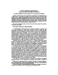
Surface Lead Break Source Several different AE source and receiver positions were used to investigate A 0 Lamb mode AE signals and their reflections generated by pencil lead breaks on the plate surface. For the first case, the source and receiver were positioned as shown in Fig. 1a to allow observation of the direct arrival and normal incidence reflection of the A 0 mode. As illustrated in that figure, the 38.1 X 50.8 cm plate was used and the propagation distance
7
for the direct arrival (illustrated as path 1) was 7.62 cm. The total propagation distance for the signal reflected off of the plate back edge (path 2) was 25.4 cm. The DFEM and experimental signals are shown in Fig. 1b. Again, both were bandpass filtered from 50 to 1000 kHz. For the A0 mode, out to the 150 µs time period shown in the Fig. 1b, only the direct arrival and the backwall reflection are observed. Excellent agreement between the theoretical prediction and experimental measurement was obtained for the A 0 mode and its reflection.
Even though the surface lead break source preferentially generated the A 0 mode, a very small S0 mode component is seen in Fig. 1b prior to the arrival of the antisymmetric mode. Because of the faster velocity of the S0 mode, the signals also contain multiple reflections of this mode. However, they are much smaller in amplitude than the dominant antisymmetric mode and were not examined in detail. The S0 mode and its reflections were studied with edge lead break sources which are discussed later in this paper.
The necessity of filtering is illustrated by examining the unfiltered theoretical and experimental signals from Fig. 1b which are shown in Fig. 2. Because of the increasing amplitude of the A0 mode at longer times, which corresponds to the lower frequency arrivals, the reflections are not even apparent. The 50 kHz high pass filter enables the observation of the reflections. The lack of agreement between the experimental signal and the DFEM prediction at longer times in Fig. 2 is caused by the lack of low frequency response of the sensor below 20 kHz.
The case of reflections at oblique incidence of the A0 mode generated by a surface lead break was studied next. The source, receiver, and plate geometry are shown in Fig. 3a. These were chosen such that, after filtering, the direct arrival (path 1) and reflected signals (path 2) were not superimposed. Again, the 38.1 X 50.8 cm plate was used. The source 8
to receiver distance was 12.7 cm, and they were equidistant (15.875 cm) from the plate edge. The total propagation distance for the reflected signal was calculated to be 34.196 cm. As illustrated in the figure, the angle of incidence (and reflection) with respect to a normal to the plate edge was 21.8 degrees. The bandpass filtered finite element and experimental waveforms are shown in Fig. 3b. Again, good agreement was observed. Fig. 4 compares the theoretical and experimental signals at even longer times. Additional reflections from the other plate edges begin to arrive after 145 µs. The agreement is still quite good for these superimposed reflections.
The final surface lead break case considered was again oblique incidence reflection. However, in this case, the dimensions were chosen such that the direct arrival and the reflected signal were superimposed. Fig. 5a shows the plate geometry, and the source and receiver positions. The 26.67 X 63.5 cm plate was used and the source to receiver distance was 20.32 cm. The source and receiver were positioned 7.62 cm from the plate edge, which produced a propagation distance for the reflected signal of 25.4 cm. The angles of incidence and reflection were 53.1 degrees. The theoretical and experimental signals are shown in Fig. 5b. In this figure, the direct arrival and reflected signals are indicated with arrows labeled 1 and 2 respectively. Arrivals of additional reflections from other plate edges appear in the signal beyond 135 µs. Again, there is good agreement between the theoretical and experimental waveforms.
Edge Lead Break Source Edge lead break sources were used to preferentially generate S 0 Lamb mode AE signals and investigate their reflections. Again, the two different plate dimensions were used, along with different source and receiver positions, to observe the particular reflections of interest. The first case studied was a reflection at normal incidence. The 26.67 X 63.5 cm plate was
9
used with the source positioned midplate along the longer edge. The positions of the source and receiver with respect to the plate dimensions are shown in Fig. 6a. Likewise, the ray paths for the direct and reflected signal are indicated in this figure as 1 and 2 respectively. The propagation distance for the direct signal was 11.43 cm, with the backwall reflection propagation distance being 41.91 cm. The bandpass filtered (100 - 750 kHz) theoretical and experimental signals are shown in Fig. 6b with the direct and reflected signal arrivals indicated by 1 and 2, respectively. As can be seen, the signals are in good agreement, with the exception of the circled A0 component in the experimental waveform, which is discussed below. Fig. 7 shows the same two waveforms with an expanded time scale so that the excellent agreement of the reflected components is more clearly seen.
As mentioned previously, it was impossible to exactly center the edge break source at the midplane of the plate. A magnifying glass and a finely ruled scale on the plate edge were used to more closely position the source at the midplane. However, an A0 mode component was always detected in the experimental signal. Several breaks were performed for all of the edge break experiments and signals were selected which contained a minimum of this antisymmetric mode component. The 100 kHz high pass filtering then eliminated most of this mode. However, as seen in the circled region of the experimental waveform in Fig. 6b, the A0 mode does contain higher frequencies which were not filtered. These are superimposed on the direct arrival of the S 0 mode. Other signals from edge lead break sources shown later in this paper also show this effect. Since the DFEM allowed the source to be positioned exactly at the midplane, a corresponding antisymmetric mode component in the theoretical signal is not observed. Fig. 8 shows the unfiltered experimental and theoretical waveforms for the source, receiver, and plate geometry shown in Fig. 6a. The unfiltered larger amplitude A0 mode in the experimental signal is clearly seen.
10
For the case of oblique incidence reflection of the S0 Lamb mode, an edge break source on the 38.1 X 50.8 cm plate was used. As shown in Fig. 9a, the source was positioned at 15.24 cm from one corner. This position was used so that the reflection from only one side could be obtained unobstructed by reflections from the back wall or other side. Also shown in Fig. 9a are the positions of the source and the ray paths for the direct (1) and reflected (2) signals. The distance from source to receiver for the direct arrival was 7.62 cm, and for the reflected signal, 31.42 cm. The angles of incidence and reflection for this reflection with respect to the normal to the plate edge were 14°. The bandpass filtered experimental and DFEM predicted waveforms are shown in Fig. 9b. This figure shows the signals out to time in which only these two arrivals (direct and sidewall reflection) are present. Very good agreement between the DFEM and experimental waveforms is demonstrated. The discrepancy of the presence of some higher frequency components of the A0 mode of the experimental signal is again noted.
If the time scale for Fig. 9b is lengthened as shown in Fig. 10b, arrivals of two additional signals are noted and are labeled 3 and 4. The arrival times for signals 3 and 4 were found to be too early to have been created by reflections from either the back edge or the far side edge of the plate. These two signals are particularly interesting in that they appear to be reflected with paths as shown in Fig. 10a, and have mode converted at the edge and corner of the specimen, respectively. Several aspects of the DFEM model signals were examined to reach this conclusion. These included the arrival times and amplitudes of signals 3 and 4 at different sensor locations, as well as the in-plane displacement components for positions along propagation paths to the edge and the corner.
The sensor locations, for which the arrival times and amplitudes were measured from the DFEM signals (equivalent to those of signals 3 and 4 in Fig. 10b), are shown in Fig. 11a. These locations were such that the direct path from the source to the sensor ranged from 11
7.62 cm to 17.78 cm in 2.54 cm intervals. Because of the smaller amplitude of arrivals 3 and 4 and their superposition with higher frequency components of other smaller arrivals, it was not possible to determine their exact first arrival time. Instead, the arrival times of the peaks of signals 3 and 4 were measured at the different locations. These arrival times were compared to those calculated using the known shear (3100 m/s) and Rayleigh velocities (2894 m/s), and the plate theory extensional velocity (5403 m/s), which approximates the earliest arrival for the S 0 mode. In comparison with the calculated arrival times, it was expected that the values measured from the peaks of the DFEM signals 3 and 4 would be slightly later. However, this time difference between measured and calculated arrivals should be constant for the different sensor locations. For signal 3, the propagation path and modes which gave a constant difference in arrival times between calculated and measured values for the different sensor locations, was that of a bulk shear wave propagating out to the edge, mode converting to a longitudinal wave with the appropriate change in angle, and then returning to the receiver as the S 0 mode. Fig. 11b shows the time difference between the measured peak of signal 3 arrival time, and the calculated arrival for this mode converted reflection. Other possible paths were considered including shear and Rayleigh waves propagating along the edge which mode convert at the corner and return as the S0 mode, and a shear mode which mode converted at the edge without the expected change in angle of reflection. None of these gave expected arrival times consistent with those measured for signal 3 at the different sensor locations.
In addition to the arrival time, the amplitude of this signal component was also measured at the various source to sensor distances. These were examined and compared to expected changes in amplitude for mode converted longitudinal waves as a function of the angles of incidence of the shear mode as discussed by Graff (1991). At the 7.62 cm distance used for the signals in Fig. 10b, the angle of incidence for the shear mode with respect to the normal to the edge is 9.34°, and the angle of reflection for the mode converted wave is 12
18.55°. The total propagation distance is 31.5 cm. The amplitude of this mode converted reflection is quite small and barely noticeable. However, if the signal is examined with the sensor at a distance of 10.16 cm from the source on the edge, the amplitude of this reflection is larger as shown in Fig. 12. In this case, the angle of incidence is 12.37° and the angle of reflection is 24.10° with a total propagation distance of 32.3 cm. Although not shown here, it was confirmed that the amplitude of this mode converted signal continues to increase if the sensor to source distance, and thus angle of incidence of shear mode, is increased. This increase of signal amplitude as a function of increasing angle of incidence is consistent with the amplitude relations for bulk shear to bulk longitudinal mode conversions. Another factor, which might also be contributing to this increase in amplitude for more distant sensor positions, is the shape of the radiation patterns for shear modes from a point monopole source, as discussed by Scruby (1985). For such a mode conversion to occur at the plate edge, it is noted that the shear wave must be polarized vertically with respect to the plate edge. Such a shear mode would then be polarized horizontally with respect to the plane of the plate. The in-plane displacements, perpendicular to the propagation direction, were also examined to evaluate the existence of a shear mode with horizontal (with respect to the plane of the plate) polarization. These were examined at the modeled sensor locations, as well as at positions along the path of the shear wave which would propagate out to the plate edge, mode convert and return to the sensor at 7.62 cm distance from the source. For the DFEM signals which propagated along a direct path to the modeled sensor locations, no transverse, in-plane displacements corresponding to an arrival of the shear mode were observed. This is to be expected if the radiation patterns, as discussed by Scruby (1985), for shear modes from a point monopole source are considered. Shear modes from such a source radiate out at angles with respect to the direction of the monopole with no component propagating directly along the direction of the monopole. The transverse, in-plane displacements for propagation along the
13
direction of the shear wave to the edge did show an arrival that corresponded to the shear wave arrival time. However, analysis of these in-plane displacement components was complicated because of other shear modes with different polarizations, and their interactions with the plate surfaces.
A similar analysis of the arrival times of the signals designated by 4 in Fig. 10b and 12 at different propagation directions was completed. From this, the path and modes of signal 4 were found to be consistent with a Rayleigh wave propagating away from the source on the plate edge, which mode converted at the plate corner and propagated to the modeled sensor location as the S0 mode. The in-plane (and normal to the plate edge) displacement from the DFEM model was examined at multiple locations along the plate edge to verify the existence of a Rayleigh wave. Fig. 13 shows the in-plane displacement component for a position at the midplane of the plate and on the edge at a distance of 7.62 cm. from the edge lead break source. The large amplitude Rayleigh wave is clearly present in this signal. The dynamics of this mode conversion at the corner are not as well understood. However, the agreement between the DFEM and experiment is again quite good for these mode converted reflections.
SUMMARY AND CONCLUSIONS The results of this study validate the three-dimensional dynamic finite element method (DFEM) for predicting AE waveforms in finite plates including reflection components. Simulated AE sources (lead breaks) were modeled and used for the experimental confirmation. Lead breaks on both the surface and the edge of thin aluminum plates were considered. In thin plates, surface lead breaks preferentially generate the A 0 Lamb mode while those on the edge near the midplane of the plate preferentially generate the S 0 mode. It was demonstrated theoretically and experimentally that the edge break source also 14
generates a Rayleigh wave which propagates along the plate edge. This Rayleigh wave interacts at the plate corner to produce a mode converted S 0 wave. Also observed theoretically and experimentally was a mode converted reflection caused by shear waves generated by the edge break source. Upon reflection, these waves mode converted at the sides of the plate to longitudinal waves which then propagated through the thin plate as the S0 mode. An absolutely calibrated, wideband sensor was used for all experimental measurements. In all cases, good agreement was obtained between the DFEM predictions and experimental measurements.
The validation of the DFEM for predicting reflections of AE signals in plates is an important step toward making it a useful tool for predicting AE waveforms in real practical structures. In such structures, signal reflections often significantly contribute to the waveform because of structural complexities such as holes, free edges, welds, joints, etc. The effect of reflections on AE waveforms is even more pronounced in laboratory specimens such as coupons, which usually have very small lateral dimensions. Further work is necessary, however, to validate the model for predicting waveforms in other practical situations to include specimens with changes in thickness, welds, and varying and/or anisotropic material properties.
REFERENCES F. Breckenridge, T. Proctor, N. Hsu, S. Fick, and D. Eitzen (1990), “Transient Sources for Acoustic Emission Work,” Progress in Acoustic Emission V, eds. K. Yamaguchi et al., JSNDI, Tokyo, pp. 20-37. J. Gary and M. A. Hamstad (1994), “On the Far-field Structure of Waves Generated by a Pencil Lead Break on a Thin Plate, J. Acoustic Emission, 12(3-4), 157-170. D. Guo, A. Mal, and K. Ono (1996), “Wave Theory of Acoustic Emission in Composite Laminates,” J. Acoustic Emission, 14(3-4), S19-S46. M. R. Gorman (1991), “Plate Wave Acoustic Emission,” J. Acoust. Soc. Am., 90(1), 358-364. 15
M. R. Gorman and W. H. Prosser (1991), “AE Source Orientation by Plate Wave Analysis,“ J. Acoustic Emission, 9(4), 283-288. M. R. Gorman and W. H. Prosser (1996), “Application of Normal Mode Expansion to Acoustic Emission Waves in Finite Plates”, J. Appl. Mech., 63(2), 555-557. K. F. Graff (1991), Wave Motion in Elastic Solids, Dover Publications Inc. (New York), M. A. Hamstad, J. Gary, and A. O’Gallagher (1996), “Far-field Acoustic Emission Waves by Three-Dimensional Finite Element Modeling of Pencil-Lead Breaks on a Thick Plate,” J. Acoustic Emission, 14(2), 103-114. M. A. Hamstad, J. Gary, A. O’Gallagher (1998a), “On Wideband Acoustic Emission Displacement Signals as a Function of Source Rise-Time and Plate Thickness,” to be published in the Proceedings of the 14’th International Acoustic Emission Symposium and 5’th Acoustic Emission World Meeting. M. A. Hamstad, J. Gary, A. O’Gallagher (1998b), “Modeling of Buried Acoustic Emission Monopole and Dipole Sources with a Finite Element Technique,” to be submitted. W. Huang (1998), “Application of Mindlin Plate Theory to Analysis of Acoustic Emission Waveforms in Finite Plates,” to be published in the Proceedings of the Review of Progress in Quantitative Nondestructive Evaluation, 17. H. Kolsky (1953), Stress Waves in Solids, Dover, New York. W. H. Prosser, M. A. Hamstad, J. Gary, and A. O’Gallagher (1998), “Comparison of Finite Element and Plate Theory Methods for Predicting Acoustic Emission Waveforms,” Submitted to the Journal of Nondestructive Evaluation. C. B. Scruby (1985), “Quantitative Acoustic Emission Techniques”, Nondestructive Testing Vol. 8, (Academic Press, Inc., London) 141-208.
16
25.4 cm Backwall 8.89 cm
2 Receiver
7.62 cm
1 X Source
38.1 cm
50.8 cm a) 0.6 Theoretical Displacement (nm)
0.4 0
Exp. 0.2 1 0
2
Theory
-0.2
-0.4
Experimental Displacement (nm)
0.2
-0.2 -0.6 0
50
100 150 Time (µs) b) Fig. 1 Direct arrival and reflection at normal incidence of A 0 Lamb mode AE signal generated by surface lead break source - a) Plate geometry and source/receiver locations, b) Filtered experimental and finite element predicted waveforms. 17
Theoretical Displacement (nm)
10
15
5
10
0
Exp.
5
-5
0
-10
Theory
-5
-15
-10
-20 0
50
100
Experimental Displacement (nm)
20
150
Time (µs) Fig. 2 Unfiltered theoretical and experimental signals for plate, source, receiver geometry shown in Fig. 1a)
18
19.05 cm
12.7 cm
19.05 cm
2
2
X Source
1 Receiver
15.875 cm
38.1 cm
50.8 cm a) 0.6 Theoretical Displacement (nm)
0.4 0
Exp. 0.2
1
0
2
-0.2
Theory
-0.4
Experimental Displacement (nm)
0.2
-0.2 -0.6 0
50
100
150
Time (µs) b) Fig. 3 Direct arrival and oblique incidence reflection of A0 mode AE signal generated by surface lead break source - a) Plate geometry and source/receiver locations, b) Filtered experimental and finite element predicted waveforms. 19
0.6 Theoretical Displacement (nm)
0.4 0
Exp. 0.2
-0.2 0
Theory
-0.4
Experimental Displacement (nm)
0.2
-0.2 -0.6 0
50
100 Time (µs)
150
200
Fig. 4 Theoretical and experimental signals from Fig. 3b over longer time scale showing good agreement for arrival of multiple reflections.
20
21.59 cm
20.32 cm 2
7.62 cm
21.59 cm 2
X Source
Receiver
1
26.67 cm 19.05 cm
63.5 cm a)
0.6
0.4 0
Exp. 0.2 1
2 -0.2
0
Theory -0.4
Experimental Displacement (nm)
Theoretical Displacement (nm)
0.2
-0.2
0
50
100 Time (µs) b)
150
-0.6 200
Fig. 5 Direct arrival and oblique incidence reflection of A0 Lamb mode AE signal generated by surface lead break source - a) Plate geometry and source/receiver locations, b) Filtered experimental and finite element predicted waveforms.
21
31.75 cm
2 26.67 cm Receiver 11.43 cm
1 Source 63.5 cm a) 0.08
0.04 Antisymmetric Mode
Theoretical Displacement (nm)
0.02
0.04
0
Exp.
0.02
2
1
0
-0.02 -0.04
Theory
-0.02
-0.06
-0.04
-0.08 120
0
20
40
60 Time (µs)
80
100
Experimental Displacement (nm)
0.06
b)
Fig. 6 Direct arrival and normal incidence reflection of S 0 Lamb mode AE signal generated by edge lead break source - a) Plate geometry and source/receiver locations, b) Filtered experimental and finite element predicted waveforms.
22
0.02 0.015
DFEM Experiment
Displacement (nm)
0.01 0.005 0 -0.005 -0.01 -0.015 -0.02 80
90
100 Time (µs)
110
120
Fig. 7 Signals from Fig. 6 with expanded time scale to compare reflected signals.
23
0.3
0.2 0
Exp. 0.1
-0.1 0
Theory -0.2
Experimental Displacement (nm)
Theoretical Displacement (nm)
0.1
-0.1 -0.3 0
50
100
150
Time (µs) Fig. 8 Theoretical and experimental waveforms from Fig. 6 prior to bandpass filtering.
24
15.24 cm
38.1 cm
Receiver
2 7.62 cm
2
1 Source 50.8 cm a)
0.08
0.04
Theoretical Displacement (nm)
0.02
0.04
0 1
0.02
2
-0.02
0
-0.04 Theory
-0.02
-0.06
-0.04
Experimental Displacement (nm)
Experiment
0.06
-0.08 0
10
20
30 40 Time (µs)
50
60
70
80
b) Fig. 9 Direct arrival and oblique incidence reflection of symmetric Lamb mode AE signal generated by edge lead break source - a) Plate geometry and source/receiver locations, b) Filtered experimental and finite element predicted waveforms.
25
15.24 cm
38.1 cm
Receiver 7.62 cm
3
4 3 Source 50.8 cm
4
a) 0.08
0.04
Theoretical Displacement (nm)
0.02
0.04
0
0.02
3
-0.02
4
0
-0.04 Theory
-0.02
-0.06
-0.04
Experimental Displacement (nm)
Experiment
0.06
-0.08 0
20
40 60 Time (µs)
80
100
b) Fig. 10 a) Plate geometry, source/receiver locations, and propagation paths for mode converted Rayleigh and shear waves, b) Filtered experimental and finite element predicted waveforms.
26
15.24 cm
38.1 cm Receivers (2.54 cm vertical spacing) 7.62 cm
3
4 3 Source 50.8 cm
4
Arrival Time Difference (µ s) DFEM Peak - Calculated
8
a)
6
4
2
0 6
8
10 12 14 16 Source to Sensor Distance (cm) b)
18
Fig. 11 a) Source and receiver positions for arrival time measurements to evaluate propagation paths for mode converted reflected arrivals b) Difference in arrival time between that measured from peak of signal 3 (DFEM) and calculated from shear/longitudinal mode converted propagation path using shear and extensional plate velocities.
27
0.08
0.04
Theoretical Displacement (nm)
0.02
0.04
0
0.02
3
-0.02
4
0
-0.04 Theory
-0.02
-0.06
-0.04
Experimental Displacement (nm)
Experiment
0.06
-0.08 0
20
40 60 Time (µs)
80
100
Fig. 12 Filtered experimental and finite element predicted waveforms for source, receiver, and plate geometry as in Fig. 10 a) except with receiver positioned at 10.16 cm propagation distance from source.
28
Theoretical Displacment (nm)
0.5
0
-0.5
-1
-1.5
-2 0
5
10
15 20 Time (µs)
25
30
35
Fig. 13 Theoretical in-plane displacement for position at midplane of plate edge at a distance of 7.62 cm from edge break source showing Rayleigh wave component arrival.
29