JAVA PERFORMANCE IN FINITE ELEMENT COMPUTATIONS G.P. NIKISHKOV University of Aizu Aizu-Wakamatsu, Fukushima 965-8580, Japan email:
[email protected] ABSTRACT 1 The performance of the developed Java finite element code is compared to that of the C finite element code on the solution of three-dimensional elasticity problems using Intel Pentium 4 computer. Untuned Java code is approximately two times slower then analogous C code. It is shown that code tuning with the use of blocking technique can provide Java/C performance ratio 90% for the LDU solution of finite element equations. Java performance for PCG iterative solution algorithm tuned by inner loop unrolling is 75% of the C code. We recommend using Java Virtual Machine JVM 1.2 since in many cases it is considerably faster in finite element computations than JVMs 1.3 and 1.4. KEY WORDS Finite Element Methods, Java-based Simulation, Performance, Tuning
1 Introduction Finite element codes were traditionally developed in Fortran [1] and recently in Fortran 90 [2]. During last decade FEM developers started using C++ language in order to handle complexity in finite element software [3-5]. Using the object-oriented approach with data hiding, encapsulation and inheritance, allows creating reliable and extensible finite element codes. Java language [6] developed by Sun Microsystems possesses features, which makes it attractive for using in computational modelling. Java is a simple language with rich collection of libraries implementing various APIs (Application Programming Interfaces). With Java it is easy to create Graphical User Interfaces and to communicate with other computers over a network. Java has built-in garbage collector preventing memory leaks. Another advantage of Java is its portability. Java Virtual Machines (JVM) [7] are developed for all major computer systems. JVM is embedded in most popular Web browsers. Java applets can be downloaded through the net and executed within Web browser. While object-oriented programming can be done with C++ language, other useful features such as actual portability and garbage collection are unique characteristics of Java language. 1 Applied Simulation and Modeling, Procs of the 12th IASTED Int. Conf., Sept. 3-5, 2003, Marbella, Spain., ACTA Press, Anaheim, 2003, pp. 130-135.
Despite its attractive features, Java is not widely used in engineering computations. Java byte code translation into native instructions leads to a slower operation of Java code. However, Just-In-Time compiler (JIT) can significantly speed up the execution of Java applications and applets. The JIT, which is an integral part of the JVM takes the bytecodes and compile them into native code before execution. Since Java is a dynamic language, the JIT compiles methods on a method-by-method basis just before they are called. If the same method is called many times or if the method contains loop with many repetitions the effect of re-execution of the native code can make the performance of Java code acceptable. Java performance in numerical computing was considered in several publications [8-10]. It was shown that high-performance numerical codes could be developed in Java with suitable code development techniques. While papers [8-10] deal with general issues of numerical computing, this paper addresses Java performance and tuning in finite element computations. We present our experience in designing the efficient finite element code in Java. The performance of the developed Java finite element code is compared to that of the analogous C code on finite element solutions of three-dimensional elasticity problems using Intel computer. For running Java code we employed Sun JVMs 1.2, 1.3 and 1.4. It is shown that with proper coding and JVM selection the Java finite element code can be almost as fast as the C code.
2
Java Finite Element Code
Object-oriented approach is used widely in order to create reusable, extensible, and reliable components, which can be used in later research and practical applications. However, full object-oriented programming approach might not be always ideal for computationally intensive sections of codes. Object creation and destruction in Java are expensive operations. The use of large amount of small objects can lead to considerable time and space overhead. As experiments show, a possible way to increase computing performance is reducing expenses for object creation in the code by using primitive types in place of objects. For a variable of a primitive type the JVM allocates the variable directly on the stack (local variable) or within the memory used for the object (member variable). For such variables there is no object creation overhead, and no
class JFem – main class controlling FEM solution interface CNST – collection of constants used during solution class Element – abstract finite element class Element2D8N – 2D quadrilateral 8-noded element class Element3D20N – 3D hexahedral 20-noded element class FiniteElementModel - description of the finite element model class LoadVectorAssembler – boundary conditions for the finite element model class Material – abstract material model class ElasticMaterial – material model for elasticity problems class DataFileReader – reading data file class Solver – abstract finite element solver class ProfileLDUSolver – solution of the finite element equation system by the direct LDU method with profile storage of the matrix class SparseRowPCGSolver - solution of the finite element equation system by the preconditioned conjugate gradient method class Node – abstract node of the finite element model class Node2D – node of the 2D finite element model class Node3D – node of the 3D finite element model
Figure 1. Class hierarchy of the JFEM code.
garbage collection overhead. Java does not support true multi-dimensional arrays. Because of this it is more appropriate to employ one-dimensional arrays even in the cases where two-subscript notation is used in the mathematical formulation of the problem. It should be noted that computationally critical code sections are small in comparison to the whole code. The whole finite element code can be designed with objectoriented approach. A compromise between using objects and providing high efficiency should be found for the computationally intensive sections of the code. Keeping in mind the above efficiency considerations we developed the Java finite element code JFEM for the solution of two-dimensional and three-dimensional elasticity problems. The class hierarchy of the JFEM code is presented in Fig. 1. The class design allows extensibility of the code. Abstract classes are used for the definition of classes for nodes, finite elements, material models and equation solvers. The abstract class defines the overall structure of the hierarchy. It contains the data members and member methods. Some methods can be implemented in the abstract class; other methods are implemented in class, which is lower in the hierarchy. For example, abstract class Element contains methods for data manipulations (connectivity data and nodal data), which are common to all element types. Methods for computing shape functions, derivatives of shape functions, element stiffness matrix, element load vector etc. are implemented in classes Element2D8N and Element3D20N for the two-dimensional 8-node element and for the three-dimensional 20-node element. It is worth noting that we try to restrict using objects in computationally intensive parts of the finite element procedure. Class
Node is used during input of the nodal data for the finite element model. During calculation of the element stiffness matrices and during the assembly and solution of the equation system only primitive types and one-dimensional arrays are used in operations with nodal data.
3
Assembly and Solution of Equation System
For linear problems main fraction of computing time is related to calculation of element stiffness matrices, assembly of the equation system and its solution. Here we present algorithms of element stiffness matrix computation and consider two algorithms of equation solution: direct method of decomposition into lower, diagonal and upper matrix (LDU) and iterative preconditioned conjugate gradient (PCG) method.
3.1
Stiffness Matrix Assembly
A global stiffness matrix of the structure is assembled of element stiffness matrices. Coefficients of the element stiffness matrix [k] are expressed as follows: Rh mn m ∂Nn kii = (λ + 2µ) ∂N ∂xi ∂xi V ´i ³ ∂Nm ∂Nm ∂Nm ∂Nm + dV, +µ ∂x ∂x ∂x ∂x i+1 i+1 i+2 i+2 mn kij
=
´ R ³ ∂Nm ∂Nn m ∂Nn λ ∂xi ∂xj + µ ∂N dV. ∂xj ∂xi
V
Here m, n are local node numbers; i, j are indices related to coordinate axes (x1 , x2 , x3 ). Cyclic rule is employed in the above equation if coordinate indices become greater
than 3. Material parameters λ and µ are Lame elastic constants. In our computer code integration of the stiffness matrix [k] for the 20-node element is performed using special 14-point integration rule. Since the element stiffness matrix possesses symmetry property, only symmetrical part of the matrix and diagonal coefficients are computed and then used for assembly of the global stiffness matrix. Assembly of the global stiffness matrix is performed with the use of element connectivity information. Assembly algorithm depends on the storage format for the finite element equation system.
3.2 LDU Solution of Equation System Symmetric part of the global stiffness matrix of the order n is stored in a profile form by columns. Each column of the matrix starts from the first top nonzero element and ends at the diagonal element. The matrix is represented by two arrays: one-dimensional double array a, containing matrix elements and a pointer array pcol. Assuming that array indices begin from one, the ith element of pcol contains the index in the array a of the first element of the ith column minus one. The length of the ith column is given by pcol[i+1]-pcol[i]. The length of the array a is equal to pcol[n+1]. The location (row number) of the first nonzero element in the ith column of the matrix [A] is given by the function FN(i):
FN(i)=i-(pcol[i+1]-pcol[i])+1. The following correspondence relation can be easily obtained for a transition from two-index matrix notation to one-dimensional array notation: a[i,j] → a[i+pcol[j+1]-j]. Solution of a symmetric equation system consists of [U ]T [D][U ] decomposition of the system matrix followed by forward reduction and backsubstitution for the righthand side. The [U ]T [D][U ] decomposition takes majority of the computing time. The right-looking algorithm of the decomposition can be presented as the following pseudocode: do j=2,n Cdivt(j) do i=j,n Cmod(j,i) end do end do do j=2,n Cdiv(j) end do
Cdivt(j) = do i=FN(j),j-1 t[i] = a[i,j]/a[i,i] end do Cmod(j,i) = do k=max(FN(j),FN(i)),j-1 a[j,i] -= t[k]*a[k,i] end do Cdiv(j) = do i=FN(j),j-1 a[i,j] /= a[i,i] end do
Do loop, which takes most time of LDU decomposition is contained in the procedure Cmod(j,i). One column of the matrix is used to modify another column inside inner do loop. Two operands should be loaded from memory in order to perform one Floating-point Multiply-Add (FMA) operation. Data loads can be economized by tuning with the use of blocking technique. After unrolling two outer loops, the tuned version of the LDU decomposition is as follows: do j=1,n,d Bdivt(j,d) do i=j+d,n,d BBmod(j,i,d) end do end do do j=2,n Cdiv(j) end do
Bdivt(k,d) = do j=k,k+d-1 do i=FN(k),j-1 t[i,j] = a[i,j]/a[i,i] end do do i=j,k+d-1 do l=max(FN(j),FN(i)),j-1 a[j,i] -= t[l,j]*a[l,i] end do end do end do
BBmod(j,i,d=2) = do k=max(FN(j),FN(i)),j-1 a[j,i] -= t[k,j]*a[k,i] a[j+1,i] -= t[k,j+1]*a[k,i] a[j,i+1] -= t[k,j]*a[k,i+1] a[j+1,i+1] -= t[k,j+1]*a[k,i+1] end do if j>=FN(j) then a[j+1,i] -= t[j,j+1]*a[j,i] a[j+1,i+1] -= t[j,j+1]*a[j,i+1] end if
Method BBmod(j,i,d) performs modification of a column block, which starts from column i by a column block, which starts from column j and contains d columns. The pseudo-code above is given for the block size d = 2 for brevity. In three-dimensional problems, which are solved here, the block size d = 3 is used. It is assumed that columns in the block start at the same row of the matrix a. This is fulfilled automatically if the column block contains columns, which are related to one node of the finite element model.
3.3
PCG Solution of Equation System
Preconditioned conjugate gradient (PCG) method is an iterative procedure, which does not alter the equation matrix. Because of this, only nonzero coefficients of the finite element global stiffness matrix can be stored. Sparse structure of the matrix should be taken into account in matrix-vector multiplications. We use sparse row format for the equation matrix. In this format all information about matrix is contained in three arrays: a - array of doubles containing non-zero elements of the matrix, row by row; col - array of column indices for non-zero elements of the array a;
prow - pointer array of indices of starting elements of matrix rows in the array a, again assuming that indices start from one. Preconditioning techniques are not the subject of this work. Simple diagonal preconditioning is used in our PCG solution procedure of finite element equations. The most time consuming operation in the PCG solution procedure is the sparse matrix-vector product inside iteration loop. Matrixvector multiplication for matrix [A] in sparse-row format is performed as follows: do j=1,n y[j] = 0 do i=prow[j],prow[j+1]-1 y[j] = y[j] + a[i]*x[col[i]] end do end do
Experience with tuning C codes shows that little can be done to speed up sparse matrix-vector product. To our surprise the following simple inner loop unrolling may improve Java code performance:
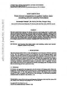
Figure 2. Finite element mesh of 8 × 8 × 8 brick-type 20node elements. 1.50 Assembly of profile system, Pentium 4 2.8GHz 1.25 1.00
tC/tJava
do j=1,n y[j] = 0 do i=prow[j],prow[j+1]-1,3 y[j] = y[j]+a[i]*x[col[i]] +a[i+1]*x[col[i+1]]+a[i+2]*x[col[i+2]] end do end do
0.75 0.50
Experiments with unrolling the outer loop lead to slower calculations. The speed up of the sparse matrix-vector product after inner loop unrolling and lack of it after outer loop unrolling can be explained by the internal compilation features of the Java compilers.
4
Experimental Results
We compared our C and Java implementations of the finite element method on the series of three-dimensional elasticity problems. The test problem is simple tension of an elastic cube. Three-dimensional meshes of E × E × E bricktype 20-node elements are used for C-Java benchmarking. The value of E varies from 4 to 14 thus providing meshes from 64 elements (1275 degrees of freedom) to 2744 elements (38475 degrees of freedom). The mesh with E = 8 is shown in Fig. 2. Desktop computer with Intel Pentium 4 2.80GHz processor (533 MHz frontside bus and 512 KB L2 cache) was used for running the C and the Java finite element codes. The C code was compiled using Microsoft Visual C++ 6.0 with maximum speed optimization. The Java code was compiled using javac compiler developed by Sun Microsystems with optimization option -O and run using Java virtual machine (JVM). Three JVMs were used: JVM 1.2.2-015 with Symantec Just-In-Time compiler; Java HotSpot Client VM 1.3.1 07-b02;
JVM 1.2 JVM 1.3 JVM 1.4
0.25
0
10
20
Number of DOF, 103
30
40
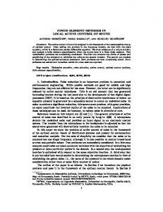
Figure 3. Ratio of the C code time to the Java code time for assembly of the global stiffness matrix in the profile format.
Java HotSpot Client VM 1.4.1 02-b06. Results for assembly of the global stiffness matrix in the profile format and for the LDU solution of the equation system are presented in Figures 3-4. Since it is difficult to determine megaflops rate for the assembly phase we present C/Java performance comparison as ratios of computing time used by the C code to computing time used by the Java code. Assembly of the stiffness matrix in the profile format is faster with JVM 1.2 than with C code. Performance of JVMs 1.3 and 1.4 is around 75% of the C code performance. Fig. 4 shows megaflops rates for the LDU solution of the equation system stored in the profile format. Untuned version of the Java code produces approximately same speed of calculation for all JVMs. Java performance of the untuned code is roughly 40% of C performance. Tuning of C and Java codes changes the performance ratios
800
1200
Untuned LDU solution, Pentium 4 2.8GHz JVM 1.2 JVM 1.3 JVM 1.4 MSC
1000 800
MFlops
600
MFlops
Tuned LDU solution, Pentium 4 2.8GHz
400
600 400
JVM 1.2 JVM 1.3 JVM 1.4 MSC
200 200
0
10
20
3 Number of DOF, 10
30
40
0
0
10
20
Number of DOF, 10
3
30
40
(b)
(a)
Figure 4. Java and C Megaflops rates for the LDU solution before tuning (a) and after tuning (b).
1.50 1.25
Assembly of sparse row system Pentium 4 2.8GHz
tC/tJava
1.00 0.75 0.50
JVM 1.2 JVM 1.3 JVM 1.4
0.25
0
10
20
Number of DOF, 103
30
40
Figure 5. Ratio of the C code time to the Java code time for assembly of the stiffness matrix in the sparse row format.
dramatically (Fig. 4,b). JVM 1.2 shows computing rates, which are around 90% of the C code rates. JVMs 1.3 and 1.4 produces lower speed for the tuned LDU code. Significant performance drops are observed for the tuned LDU code when using JVM 1.3. Such phenomena can be explained by data block conflicts in cash memory for certain profiles of the equation system. Fig. 5 presents comparison of C and Java speeds for the assembly of the global stiffness matrix in the sparse row format. JVM 1.2 produces best speed. The speed of Java code run with JVM 1.2 is higher than the C code speed. Lower speeds are shown by JVMs 1.3 and 1.4 (60% of the C speed). Megaflops rates for the PCG solution of equation system are depicted in Fig. 6. For the untuned PCG solution,
Java is about two times slower then C. Tuning does not affect the speed of the C code. However, simple code tuning with unrolling only inner loop of the sparse matrix-vector product improves Java performance considerably making the Java speed equal to 75% of the C speed. There is a recommendation [9] to use JVM 1.4 and to run it with the -server option in order to increase speed of the Java codes. Our attempts to do so showed that the finite element computations are 20% slower with the -server option in comparison to the default -client option. The data presented in Figs 3-6 shows performance results for the three types of computations: 1) Calculation of element stiffness matrices and assembly of the global stiffness matrix: mostly computations with scalar variables; 2) LDU solution of the equation system: mostly triple loop for multiply-add operations for columns with a consecutive access to operands; 3) PCG solution of the equation system: mostly double loop for multiply-add operations with a nonconsecutive access to operands. The experimental results show that the performance of Java is on par with C for computations involving mostly scalar variables. For multiply-add operations with the consecutive access to array elements inside the triple loop the Java performance can be 90% of the C performance after tuning. For multiply-add operations with the non-consecutive access to array elements inside double loops, the Java performance is 75% of the C performance. It should be noted that this conclusion is true if the proper choice of the Java machine is done (JVM 1.2). While it is reasonable to use the latest Java SDK (Software Development Kit) for most purposes, we can recommend also to install Java Runtime
600
600
Untuned PCG solution, Pentium 4 2.8GHz
Tuned PCG solution, Pentium 4 2.8GHz
500
500 400
JVM 1.2 JVM 1.3 JVM 1.4 MSC
300
MFlops
MFlops
400
300
200
200
100
100
0
10
20
3 Number of DOF, 10
30
40
0
(a)
JVM 1.2 JVM 1.3 JVM 1.4 MSC 10
20
3 Number of DOF, 10
30
40
(b)
Figure 6. Java and C Megaflops rates for the PCG solution before tuning (a) and after tuning (b).
Environment JRE 1.2 and to employ it for performing large finite element analyses.
References [1] K.-J. Bathe, Finite Element Procedures (Englewood Cliffs: Prentice- Hall, 1996).
5
Conclusion
We have designed the object-oriented version of the threedimensional finite element code for elasticity problems and implemented it in Java programming language. Special attention has been devoted to the efficient implementation of computationally intensive sections of the code. The performance of the Java code has been compared to the performance of the analogous C code on the solution of three-dimensional elasticity problems using a computer with Intel Pentium 4 processor. Java Virtual Machines 1.2, 1.3 and 1.4 were used for running Java code. The experimental results show that the performance of the Java finite element code is roughly equal to the performance of the C code for calculation of element stiffness matrices and assembly of the global equation system when using JVM 1.2. JVMs 1.3 and 1.4 provide lower performance. Untuned Java code demonstrates relatively low performance for the LDU solution of the equation system in the profile format. However, tuning with blocking technique affects speed of the Java code more than speed of the C code. Performance of the tuned Java code running on JVM 1.2 is about 90% of the C code performance. The PCG iterative solution of the equation system is 30% slower using the Java tuned code in comparison to the C tuned code. It is possible to conclude that the Java language is quite suitable for development of finite element software. With the use of proper coding the performance of the Java code is comparable to the performance of the corresponding tuned C code. It is recommended using JVM 1.2 for large finite element analyses.
[2] I.M. Smith and D.V. Griffiths, Programming the Finite Element Method (Chichester: Wiley, 1998). [3] R.I. Mackie, Using objects to handle complexity in finite element software, Engineering with Computers, 13, 1997, 99-111. [4] R.I. Mackie, Object-Oriented Methods and Finite Element Analysis (Stirling: Saxe-Coburg, 2001). [5] Y. Dubois-Pelerin and P. Pegon, Object-oriented programming in nonlinear finite element analysis, Computers and Structures, 67, 1998, 225-241. [6] J. Gosling, B. Joy and G. Steele, The Java Language Specification (Reading, MA: Addison-Wesley, 1996). [7] T. Lindholm and F. Yellin, The Java Virtual Machine Specification (Reading, MA: Addison-Wesley, 1996). [8] R.F. Boisvert, J. Moreira, M. Philippsen and R. Pozo, Java and numerical computing, Computing in Science and Engineering, March/April, 2001, 18-24. [9] D. Kruger, Performance tuning in Java, Java Developers Journal, August, 2002, 44-52. [10] J.E. Moreira, S.P. Midkiff, M. Gupta, P.V. Artigas, M. Snir and R.D. Lawrence, Java programming for high-performance numerical computing, IBM Systems Journal, 39, 2000, 21-56.