18 a frequency based transit model for dynamic ... - Semantic Scholar

A frequency based transit model for dynamic traffic assignment to multimodal networks 1

18

A FREQUENCY BASED TRANSIT MODEL FOR DYNAMIC TRAFFIC ASSIGNMENT TO MULTIMODAL NETWORKS Lorenzo Meschini, Guido Gentile, Natale Papola Dipartimento di Idraulica Trasporti e Strade, Università “La Sapienza”, Rome, Italy [email protected], [email protected], [email protected]

INTRODUCTION The pricing and rationing measures applied to discourage the use of private cars, in order to alleviate the increasing road congestion and the consequent worsening pollution, are not always coupled with a consistent policy aimed at improving the performances, or at least the capacity, of the transit system. As a result, in many modern cities the problem of full transit carriers is becoming more and more relevant. Although this situation should be avoided through a correct design of the transit network by suitably increasing the line capacities, it is still important to properly simulate the current scenario in order to justify the resources needed to carry out appropriate interventions. Thus, we are interested here in modelling the dynamic behaviours of heavy congested, urban, multimodal (transit and road) networks, where the service is so irregular or so frequent that there is no point for passengers to synchronize their arrival at the stop with the scheduled time of carriers, if any is published. Within this context, we aim at properly reproducing the important dynamic congestion phenomenon of the temporary over saturation of roads and transit lines; that is, both the formation and dispersion of car and transit carrier queues on road arcs, and the formation and dispersion of passenger queues at transit stops, where passengers wait for the first run of the chosen line actually available to them. The frequency-based static assignment models commonly used to simulate and plan urban transit networks are suited to represent systems (metro, tramways, busses) where it is generally assumed that a passenger, after reaching a stop, waits for the first attractive carrier

2 Insert book title here among some common lines. This leads to the concept of optimal strategy (Spiess and Florian, 1989) which can be formally expressed in terms of a shortest hyperpath (Nguyen and Pallottino, 1988). These models allow to suitably represent the effect of congestion on travel choices and passengers flows, but cannot represent properly the dynamic congestion phenomenon introduced above. In fact, the traditional approach to reproduce this congestion phenomenon in a static framework is based on the concept of effective frequency (DeCea and Fernandez, 1993), stating that the line frequency perceived by the passengers waiting at a stop decreases as the probability of not boarding its first arriving carrier increases. Since the residual capacity of a run available to passengers waiting at the stop depends on the number of people that are already onboard, who do not experience the cost of queuing, then, in order to apply properly the effective frequency approach, an asymmetric arc cost function is to be introduced, as in Bellei et al. (2003). An alternative and well established approach to represent transit systems, which are intrinsically discrete in time, adopts a diachronic graph (Nuzzolo et al., 2003), where each run is modelled through a specific sub-graph whose nodes have space and time coordinates according to the timetable. The main advantage of transit models based on diachronic graphs lays in the fact that, even with an explicit representation of the time dimension, they can be reduced to static assignments on space-time networks. Then, a similar approach to that of effective frequency can be adopted in order to represent congestion due to limited capacity on transit carriers (Crisalli, 1999; Nguyen et al., 2001); even though this makes it possible, as in the static case, to simulate the priority of passengers onboard, a distortion on the cost pattern is introduced: at the equilibrium, the cost for the passengers who board the arriving run is equal to that suffered by those who must wait at the stop for a successive run. Moreover, when using this approach a compromise is to be made between numerical convergence and accuracy in constraint satisfaction, because, if the waiting cost increases too strongly when the onboard flow approaches the residual capacity, then the assignment algorithm becomes unstable. Finally, when applied to congested multimodal urban network, these models present some significant drawbacks: - on the supply side, diachronic graphs are not suited to represent congestion effects on travel times, since the graph structure itself must vary with the flow pattern; - on the demand side, since in urban transit networks with high frequency passengers perceive lines as unitary supply facilities, it is not necessary to represent the single runs explicitly; this circumstance is widely exploited in the existing static models for transit assignment (De Cea and Fernandez, 1993; Wu et al., 1994; Nguyen et al., 1998); - on the algorithm side, the complexity of the assignment problem increases more than linearly with transit line frequencies, due to the grow of graph dimension. These drawbacks are overcome in this paper, were we present a new model and algorithm, aimed at solving the multimodal Dynamic Traffic assignment (DTA). The proposed approach extends an existing DTA model for road networks, presented in Bellei et al. (2005) and in Gentile et al. (2006), based on a macroscopic representation of time-continuous flows. Here, the


multimodal DTA is regarded as a Dynamic User Equilibrium1 and is formalized as a system between a dynamic arc performance function and a dynamic Network Loading Map1 (NLM), thus avoiding the introduction of the Dynamic Network Loading1 (DNL) model and the need of explicit path enumeration. The equilibrium model results in a fixed-point problem in terms of arc flow and transit frequency temporal profiles, similarly to the static multimodal equilibrium model presented in Bellei et al. (2003), and is schematically depicted in Figure 1. o-d demand flows

network loading map o-d modal satisfactions

mode choice model

arc conditional probabilities

o-d modal flows

implicit path choice model

network flow propagation model transit frequency propagation model arc modal flows

arc exit times

stop transit frequencies

arc exit time model equivalent flow model

arc costs arc cost model

arc equivalent flows

arc performance function

Figure 1. Scheme of the proposed multi modal DTA model

The main innovation in the multimodal assignment model proposed here is to represent the dynamic behavior of transit supply using a frequency approach, instead of a run approach, thus not requiring a diachronic graph. By so doing, intra modal congestion effects can be efficiently and effectively simulated, particularly those produced by the capacity constraints of transit carriers, both in terms of waiting delays and passenger queues at stops. The 1

For reader’s convenience we recall that a) the Dynamic User Equilibrium is a state of the network where, at each instant, no user can reduce his perceived travel cost by unilaterally changing route, which implies that users associate to each path its actual cost (the cost that would be actually experienced travelling along the path), and then choose a minimum actual cost path between their origin and destination; b) the Network Loading Map is the problem of loading all user trips on the chosen paths yielding the arc inflows corresponding to the given arc travel time and cost pattern; c) the Dynamic Network Loading is the problem of loading the network with given path flows in such a way that the resulting arc flow temporal profiles are consistent, through an arc performance model, with the corresponding travel time temporal profiles. The latter problem, raised by the presence of the temporal dimension affecting the DTA, is so important that in the literature much attention has been devoted to its specific analysis (see, for instance, Xu et al., 1999).

4 Insert book title here proposed approach is simply to represent these phenomena within a suitable arc performance function, which yields waiting time temporal profiles, consistent with a FIFO representation of passenger queues, for any given passenger flow and transit frequency pattern. The detail of the waiting time of single runs at stops, which cannot be represented any more, is replaced here by the average line access time temporal profile, which indeed corresponds to the expected waiting time at a stop in a frequency-based transit service; this way, calculations are simplified, while no notable error is introduced when calculating waiting time temporal profiles, as it will be clarified in the algorithm section. The road congestion will be simulated with a suitable macroscopic dynamic arc performance model, such as the one presented in Gentile et al. (2005) Inter modal congestion phenomena occurring whenever cars and transit carriers share the same facility are simulated, on the road side, through the concept of equivalent flows, representing the contribution of the transit system to road congestion; on the transit side, the dependence of line carriers travel times on road traffic conditions, which may affect transit frequencies and waiting times, is reproduced introducing a new transit frequency propagation model. The demand model, based on random utility theory, has two main choice levels: mode choice (Road and Transit) and route choice. With reference to the latter, we present both a deterministic and a stochastic Logit model, based on the results presented in Gentile and Meschini (2006) and in Bellei et al. (2005), respectively; moreover, we assume a completely preventive user’s behavior. While the above model has a time continuous formulation, its numerical solution requires, as usual, a time discretization. However, a key feature of the above approach is that it does not exploit the acyclic graph characterizing the corresponding discrete-time version of the problem (Gentile et al., 2006), so that no upper bound is set on the interval length by the solution method itself; in fact, this approach is intended to work with time intervals of several minutes, and allows the modeller to choose the time discretization based on the best trade-off between results accuracy and calculation times. In summary, this model inherits from the existing dynamic traffic assignment model presented in Bellei et al. (2005) and Gentile et al. (2006) several key features, consisting in: - formalizing the problem as a system of two functionals (namely, the NLM and the arc performance function), instead of as a system of a functional and of the parametric solution to a problem (namely, the demand function and the DNL); - achieving, jointly with the equilibrium, both the temporal consistency of the supply model and the demand-supply consistency, since it is no longer necessary to achieve the first through a DNL; - formulating DTA through an implicit path approach; - the possibility of defining “long time intervals” (5-10 min), which allows overcoming the difficulty of solving DTA instances on large networks and long period of analysis; - devising, on these bases, an efficient dynamic assignment algorithm, whose complexity is equal to the one resulting in the static case multiplied by the number of long time intervals introduced. Moreover, with respects to the representation of heavy congested multi modal urban transportation systems, it presents the following advantages and innovations:


- the dynamic behavior of transit supply is represented using a frequency approach, instead of a run approach, thus not requiring a diachronic graph representation of transit supply; - intra and inter modal congestion effects can be efficiently and effectively simulated, particularly those produced by the capacity constraints of transit carriers and affecting waiting and travel times; - on the algorithm side, the complexity of the assignment problem is independent of the transit line frequencies.

MULTIMODAL NETWORK FORMALIZATION The aim of this section is twofold: firstly, we want to achieve a representation of the multimodal network such that the relations between road and transit elements, which are necessary to formalize non-separable cost functions modeling intra and inter modal congestion, can be correctly and univocally identified; secondly, we want to define the minimum amount of information needed to apply the proposed multimodal assignment model, highlighting also the operation of converting the input data, usually organized in a GIS database, into the assignment graph handled by the model. Without loss of generality, in the following we will represent two travelling modes: the road mode R and the transit mode T, and we will refer to the generic mode m∈M = {R, T}. To this end, a base network is introduced, represented by a directed graph H = (V, E), where V⊂ℵ is the set of vertices (ℵ is the set of positive integer numbers), and E⊆V×V is the set of edges. The generic edge ε is univocally identified by its initial vertex IV(ε) and its final vertex FV(ε), that is ε = (IV(ε), FV(ε)). The set of origins and destinations of passenger and car trips, referred to as centroids, is a subset Z⊆V of the vertices. The generic vertex ν∈V is associated with a location in space that can be accessed by passengers or cars, which is characterized by geographic coordinates (λν, θν)∈ℜ2 (ℜ is the set of real numbers), while the generic edge ε∈E is characterized by a length Lε∈ℜ+ (ℜ+ is the set of non-negative real numbers). Not each edge is allowed for all modes belonging to the road and transit systems (that is: pedestrians, transit carriers, private cars); therefore, three Boolean car, pedestrian, transit line allowed-edge variables CAE(ε), PAE(ε), LAE(ε)∈{0,1} are introduced, where each one is equal to 1, if the corresponding mode is allowed on edge ε∈E, and to 0, otherwise. The road network is represented associating to each edge ε: CAE(ε) = 1 an exit capacity Qε∈ℜ++ (ℜ++ is the set of positive real numbers), which is the maximum vehicular flow that can exit it, an under saturation speed Sε∈ℜ++, which is the average speed on the edge when no queue is present on it, that is its outflow is below the exit capacity, and a road fare RFε∈ℜ+, which can be time varying. The road network is also characterized by a car occupancy coefficient γ∈ℜ++, allowing to express car flows as a function of user flows.

6 Insert book title here The line network is represented by a set ℑ⊆ℵ of lines. The generic line ℓ∈ℑ is characterized, from a topological point of view, by an ordered sequence of σℓ∈ℵ progressive points, referred to as its route, each one corresponding to a different vertex: R(ℓ) = {rn(ℓ)∈ℵ: (IV(rn(ℓ)),FV(rn(ℓ)))∈E, LAE((IV(rn(ℓ)),FV(rn(ℓ))) = 1, n∈[1, σℓ]⊆ℵ} ⊆ V, where we assume that consecutive progressive points are always connected by an edge permitted for transit carriers. For any given vertex ν∈V and line ℓ∈ℑ, the function n(ν, ℓ) yields, if it exists, the index n such that rn(ℓ) = ν, and 0 otherwise. Without loss of generality, we assume that line stops lays in correspondence of progressive points; since not every progressive point is a stop, a Boolean is-a-stop variable ISnℓ∈{0,1} is introduced, that is equal to 1, if the n-th progressive point of line ℓ is a stop, and 0 otherwise. We assume that the first progressive point of a route is always a stop, that is IS1ℓ = 1. Line carriers are characterized by: - a carrier capacity Qℓ∈ℜ++, which is the nominal capacity, usually expressed by the number of available seats, if standing in the carrier is not allowed; on the contrary case, it expresses the maximum number of passengers that can physically fit in the carrier; - a boarding and alighting capacity BQℓ∈ℜ++ and AQℓ∈ℜ++, expressing the maximum flow of passengers that can get on/off the carrier; - a time needed to open and close the doors δ ℓ∈ℜ+ ; - a car equivalent coefficient λℓ∈ℜ++ , expressing the carrier contribution to road congestion in terms of an equivalent number of cars; - an operative free-flow speed Sℓ∈ℜ++ ; - an operative acceleration ACℓ∈ℜ++ ; - an operative deceleration DEℓ∈ℜ++ . Each line ℓ∈ℑ is operated with a base frequency ψℓ(τ)∈ℜ++, expressing the instantaneous carriers departure frequency from the terminal (that is from vertex r1(ℓ)) at time τ∈ℜ+. Regarding the fare schema, we attach to the n-th section of line ℓ∈ℑ, from the vertex rn(ℓ) to the vertex rn+1(ℓ), with n∈[1, σℓ-1], a specific section fare SFnℓ∈ℜ+, which can be time varying, so as to obtain purely additive path costs, which allows implicit path enumeration in route choice computations. To each mode m∈M is associated a vector of attributes Xm∈ℜ and a corresponding vector of coefficient βm∈ℜ, characterizing it with respect to the modal choice performed by users. On this basis, the formal multimodal network handled by the assignment model can be represented by a directed graph G = (N, A), where N is the set of the nodes, and A is the set of the arcs. The generic node x∈N is identified by an ordered couple, whose first element is the node line, denoted NL(x) ⊆ {0}∪ℑ, and the second element is the node vertex, denoted NV(x) ⊆ -ℑ∪ℑ, that is x = (NL(x), NV(x)). This lets us to distinguish 4 different types of nodes, as depicted in Figure 2: RN ={(0, v): v∈V} road nodes; PN = {(0, -v): v∈V} pedestrian nodes;


LN = {(ℓ, rn(ℓ): ℓ∈ℑ, n∈[2, … , σℓ] ⊆ ℵ} line nodes; ℓ QN = {(ℓ, -rn(ℓ)): ℓ∈ℑ, n∈[1, … , σℓ-1] ⊆ ℵ, ISn = 1} queuing nodes; so that we have: N = RN∪PN∪LN∪QN . As usual, the generic arc a∈A is identified by an ordered pair of nodes, referred to respectively as the tail, denoted TL(a) ⊆ N, and the head, denoted HD(a) ⊆ N; that is a = (TL(a), HD(a)). As depicted in Figure 2, we distinguish 6 different types of arcs: RA = {( (0, u) , (0, v) ): (u, v)∈E, CAE((u, v)) = 1} road arcs; PA = {( (0, -u) , (0, -v) ): (u, v)∈E, CAE((u, v)) = 1} pedestrian arcs; LA = {( (ℓ, rn(ℓ)) , (ℓ, rn+1(ℓ)) ): ℓ∈ℑ, n∈[1, σℓ-1] ⊆ ℵ} line arcs; ℓ QA = {( (0, rn(ℓ)) , (ℓ, -rn(ℓ)) ): ℓ∈ℑ, n∈[1, σℓ-1] ⊆ ℵ, ISn = 1} queueing arcs; BA = {( (ℓ, -rn(ℓ)) , (ℓ, rn(ℓ)) ): ℓ∈ℑ, n∈[1, σℓ-1] ⊆ ℵ, ISnℓ = 1} boarding arcs; ℓ AA = {( (ℓ, rn(ℓ)), (0, rn(ℓ)) ): ℓ∈ℑ, n∈[2, σℓ] ⊆ ℵ, ISn = 1} alighting arcs, so that we have: A = RA∪PA∪LA∪QA∪BA∪AA .

8 Insert book title here

(ℓ, v ≡ rn+1(ℓ))

(ℓ, z ≡ rn+2(ℓ))

(0, -u)

(0, -v)

(0, -z)

(0, u)

(0, v)

(0, z)

v

z

(ℓ, u ≡ rn(ℓ))

Line ℓ (ℓ, -u ≡ -rn(ℓ))

Multimodal graph u

Base network Vertex ∈ V

Road Node ∈ RN Pedestrian Node ∈ PN

Edge ∈ E Road Arc ∈ RA Pedestrian Arc ∈ PA Line Arc ∈ LA

Line Node ∈ LN

Queuing Arc ∈ QA

Queuing Node ∈ QN

Boarding Arc ∈ BA Alighting Arc ∈ AA

Figure 2. Generic portion of the base network and the corresponding modal graphs.

To be noticed that more than one line may stop at the same pedestrian node, and that the structure of the pedestrian network can be very simple or very complex, depending on the modeling choices; Figure 2 does not illustrate these facts. The proposed network formalization allows to define the following relation among its elements: - Each arc a∈LA∪QA∪BA∪AA is univocally associated with a line ℓ(a)∈ℑ; specifically, if a∈AA, then ℓ(a) = NL(TL(a)), otherwise ℓ(a) = NL(HD(a)). Moreover, we can denote as n(a) = n(NV(TL(a)), ℓ(a)) the index of the associated route vertex;


- each arc a∈LA is associated with the unique road arc, if exists, sharing the same edge, that is: LR(a) = {b∈RA: ( (0,VN(TL(a))) , (0,VN(HD(a))) ) = b} ⊂ RA∪∅; - each road arc a∈RA is associated with the set of line arcs sharing the same edge, that is: RL(a) = {b∈LA: ( (0,VN(TL(b))) , (0,VN(HD(b))) ) = a } ⊂ LA∪∅ ; - each arc a∈A is associated with an edge, that is ε(a) = ( VN(TL(a)), VN(HD(a)) ) Finally, we will denote with Nm⊆N and Am⊆A the subset of nodes and arcs allowed for mode m, with NT = PN∪LN∪WN, AT = PA∪LA∪QA∪BA∪AA, and NR = RN, AR = RA.

THE ARC PERFORMANCE FUNCTION We first introduce the notation for arc usage and arc performance variables: fa(τ) inflow of users on arc a∈A at time τ; ea(τ) outflow of users from arc a∈A at time τ; ta(τ), ca(τ) exit time and cost for users entering arc a∈A at time τ; n φℓ (τ) transit frequency at the n-th progressive point of line ℓ at time τ; In order to represent the inter modal congestion phenomena occurring whenever cars and transit carriers share the same facility, we introduce the equivalent inflow ua(τ) and the equivalent outflow va(τ). With reference to the generic road arc a∈AR, we assume that its equivalent flows are a linear combination of car flows and transit frequencies of those lines using it, that is: ua(τ) = fa(τ) /γ +Σb∈RA(a) λℓ(b) ⋅φℓ(b)n(b)(τ) ,

(1.a)

va(τ) = ea(τ) /γ +Σb∈RA(a) λℓ(b) ⋅φℓ(b)n(b)+1(τ) ,

(1.b)

With reference to the generic transit arc a∈AT, the equivalent flows coincide with the user flows. Relations (1) can be expressed in a compact form by the following functional, expressing the equivalent flow model: [u, v] = Υ(f, e, φ)

(2)

where the arc components of u, v, f, e and φ are temporal profiles. On this basis, the arc performance function aims at determining the travel time temporal profile and the generalized cost temporal profile on each arc of the multimodal network as a function of the equivalent inflow and outflow temporal profiles and of the transit frequency temporal profiles of the adjacent arcs. Introducing the functional Γ, the arc performance function can be thus expressed in compact form, as: [t, c] = Γ(u, v, φ)

(3)

where the arc components of t and c are temporal profiles. Functional (3) will be specified in the following sections with reference to the different arcs introduced above, so as to obtain a macroscopic arc performance function representing, with respect to the road network, the effect of limited road capacities, and with respect to the

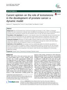
10 Insert book title here transit network, the effects of transit service discontinuity and transit carrier capacities in the context of transit line representation as continuous vehicle flows. Road arcs With reference to road arcs, functional (3) can be specified utilizing a suitable macroscopic dynamic arc performance model, such the spatially separable model presented in Gentile et al. (2005), where arc performances are evaluated through an approximate solution of the Simplified Theory of Kinematic Waves and a parabolic-triangular fundamental diagram, or such the spatially non-separable network performance model presented in Gentile et al. (2006), which extends the previous one in order to represent spillback congestion. Here, in order to focus on paper’s topics, we will specify functional (3) with reference to a simple link model, where the generic road arc a∈RA represents a road link of length Lε(a); at the final section of the link we have a bottleneck with capacity Qε(a) constant in time, strictly positive and bounded. When there is no queue, the vehicles travel along the arc with a constant under saturation speed Sε(a), so that their travel time is Lε(a)/Sε(a). When the inflow ua(τ) exceeds the exit capacity Qε(a), an over saturation queue occurs; if the queue arises at time σ + Lε(a)/Sε(a), the exit time of a vehicle entering the arc at time τ ≥ σ is equal to that time, plus the time that takes to all the vehicles that entered the arc between σ and τ to pass through the bottleneck at the maximum rate Qε(a). Based on the results achieved in Gentile et al. (2005), as depicted in Figure 3, the worst case dominates the others. Then, we have:

vehicles

⎧⎪ ⎫⎪ Lε ( a ) τ 1 ta (τ) = max ⎨σ + + ⋅ ∫ ua ( x)dx : σ ≤ τ ⎬ . Sε ( a ) Qε ( a ) σ ⎪⎩ ⎪⎭

(4)

cumulative outflow temporal profile cumulative inflow temporal profile

Qε(a)

∫

τ

σ

Lε(a)/Sε(a) σ

τ

ua (t ) ⋅ dt

time ta(τ)

Figure 3. Arc exit time for a link with fixed under saturation speed and fixed exit capacity.

This model is coherent with the simplified kinematics waves theory (Daganzo, 1997) assuming a triangular shaped fundamental diagram, like the one depicted in Figure 4; in fact, in Gentile et al. (2005) it is proved that the density and the queue speed corresponding to the


bottleneck capacity (respectively, point B' and V(Qε(a)) in Figure 4) are meaningless with respect to the arc travel times. Moreover, the model respects the non-strict version of the FIFO rule, that is: txy(τ′) ≥ txy(τ) , for any τ′ > τ .

(5) τ′ ∫τ fxy(t)

Indeed, if no vehicle enters the arc between any τ and τ′ > τ, that is ⋅ dt = 0 , while the queue is vanishing, that is txy(τ′) > τ′ + Lxy / Vxy , it results that txy(τ′) = txy(τ). flow

B

Qε(a) arctg Sε(a)

arctg V(Qε(a)) B'

density

Figure 4. The proposed link model for road arcs is coherent with a triangular fundamental diagram.

The travel cost of the generic road arc a∈RA is given by the sum of its travel time multiplied by the value of road time χ∈ℜ+, and of the proper road fare: ca(τ) = χ ⋅ (ta(τ) - τ) + RFε(a)(τ).

(6)

Queuing and boarding arcs

The queuing and boarding arcs of a given stop are aimed at representing the total waiting time suffered by a user in order to board the chosen line. In fact, when the line is congested, that is the flow willing to board is higher than the line available capacity at that stop, the waiting time results by the sum of two components, modelled respectively by the queuing arc and the boarding arc: - the over saturation waiting time, which represents the time spent by users queuing at the stop and waiting that the service become actually available to them; it can be thought as the time spent by each user waiting until the next carrier arriving at the stop will be the one he can actually board; - the under saturation delay, which represents the average delay due to the fact that the transit service is not continuously available over time; it can be thought as the additional delay suffered by each user waiting until the carrier that he will board arrives at the stop; Obviously, if the line is not congested, the over saturation waiting time is null and the total waiting time coincides with the under saturation delay.

12 Insert book title here With reference to the generic boarding arc a∈BA, the under saturation delay is evaluated assuming it proportional to the inverse of the corresponding line frequency, evaluated at the boarding instant; thus we have: ta-1(τ) = τ -αℓ(a) /φa(τ)

(7)

where ta-1(τ) is the entry time for the user exiting the arc a∈BA at time τ and αℓ(a) takes into account headway irregularity (in particular, αℓ(a) = 0.5 with uniform headway, αℓ(a) = 1 with Poissonian headway). Then, for a given entry time τ, the corresponding exit time is given by: ta(τ) = τ': ta-1(τ') = τ

(8)

and the exit time temporal profile is simply the inverse of the entry time temporal profile: t[a] = [t[a]-1]-1

(9)

With reference to the generic queuing arc a∈QA, the over saturation waiting time is evaluated by means of a bottleneck with time variable exit capacity, whose exit capacity is related to the available capacity of line ℓ(a) at progressive point n(a). At a given time τ, the available capacity is given by the line capacity at that point, depending on the carrier capacity and on the line frequency at τ, minus the flow already onboard at τ, that is: AKn(a)(τ) = Qℓ(a) ⋅φℓ(a)n(a)(τ) – [vb(τ) – uc(τ)] b∈LA: ℓ(b) = ℓ(a), n(b) = n(a) - 1 , c∈AA: ℓ(b) = ℓ(a), n(b) = n(a),

(10)

where the term in square brackets is the flow already onboard, which coincides with the onboard flow arriving at the stop minus the flow alighting at it (see Figure 2). At a given time τ, the capacity actually available at the end of the queuing arc is not the available capacity at the same time, because of the presence of the under saturation delay on the boarding arc. Then, the bottleneck exit capacity temporal profile can be obtained propagating backward in time the available capacity temporal profile accordingly with the under saturation delay, the FIFO and the capacity conservation (Cascetta, 2001), that is: ξa(tb-1(τ)) = AKn(a)(τ) /∂(tb-1(τ))/∂τ , b∈BA: TL(b) = HD(a)

(11)

Then, the problem of determining the exit time ta(τ) for a user that enters the queuing arc a∈QA at the generic time τ, in presence of a time-varying exit capacity ξa(σ) for each time σ, shall be addressed identifying firstly the cumulative exit flow temporal profile, whose value Ea(τ) at time τ is given by: Ea(τ) = min{Fa(σ) + Ξa(τ) - Ξa(σ): σ ≤ τ} ,

(12)

where Fa(τ) denotes the cumulative inflow at the generic time τ, that is the number of users that entered arc until time τ: τ

Fa (τ) = ∫ ua (σ) ⋅ dσ , −∞

and Ξa(τ) denotes the cumulative exit capacity at the generic time τ:

(13)


τ

Ξ a ( τ ) = ∫ ξ a ( σ ) ⋅ dσ .

(14)

−∞

The above expression (12) can be explained as follows. If there is no queue at a given time τ, the travel time is null and the cumulative exit flow is equal to the cumulative inflow. If a queue arises at time σ < τ , from that instant until the queue vanishes the exit flow equals the exit capacity, and then, based on the FIFO rule, the cumulative exit flow Ea(τ) results from adding to the cumulative inflow at time σ the integral of the exit capacity between σ and τ, that is Ξa(τ) -Ξa(σ). Moreover, if there is no queue at time τ , the cumulative exit flow is the same of the case when the queue arises exactly at σ = τ. The actual cumulative exit flow at time τ is the minimum among each cumulative exit flow that would occur if the queue began at any previous instant σ ≤ τ . Based on the FIFO rule, the cumulative exit flow at the exit time ta(τ) of a user that enters the arc at τ is equal to the cumulative inflow at time τ , that is: Ea(ta(τ)) = Fa(τ) .

(15)

However, in presence of intervals with null flow, the above implicit expression does not allow to obtain a univocal value of the travel time. To take this circumstances into account, once the cumulative exit flow temporal profile is known, the exit time temporal profile is calculated conventionally as: ta(τ) = max{0, min{σ: Ea(σ) = Fa(τ)}} .

(16)

Figure 5 depicts a graphical interpretation of equation (12), where the cumulative exit flow temporal profile Ea(τ) is the lower envelop of the following curves: a) the cumulative inflow Fa(τ); b) the family of functions Fa(σ) + Ξa(τ) - Ξa(σ) with τ > σ , for every time σ , each one obtained from the vertical translation of the cumulative exit capacity temporal profile that goes through the point (σ, Fa(σ)). No queue is present when curve a) prevails; therefore, the queue arises at time σ' and vanishes at time σ''. In the same framework, the calculation of the exit time based on the cumulative inflow and exit flow temporal profiles is shown using thick arrows. users Fa(τ)

Ea(τ)

Fa(σ) + Ξa(τ) - Ξa(σ), τ > σ Fa(υ) + Ξa(τ) - Ξa(υ), τ > υ Fa(σ)

Ea(σ)

Ξa(σ)-Ξa(σ')

Ea(ta(τ')) = Fa(τ')

σ'

τ'

ta(τ')

σ

Figure 5. Bottleneck with time-varying capacity.

Fa(σ') σ''

time

14 Insert book title here Finally, the cost for the generic arc a∈QA∪BA is given by its travel time multiplied by the value of waiting time μ∈ℜ+: ca(τ) = μ ⋅ (ta(τ) - τ) .

(17)

Line arcs

The exit time from the generic arc a∈LA at a given entry time τ is determined by the sum of three terms: the dwelling time at the stop DTa, the uncongested travel time URTa, and the delay CDa due to road congestion, evaluated at time τ + DTa(τ) when the carrier leaves the stop, that is: ta(τ) = τ + DTa(τ) + URTa +CDa(τ + DTa(τ))

(18)

The dwelling time is determined by the time needed for passengers to alight and to board the carrier, plus time needed to open and close the doors: ta(τ) = τ + (ub(τ) /φℓ(a)n(a)(τ)) / AQℓ(a) + (vc(τ) /φℓ(a)n(a)(τ)) / BQℓ(a) + 2 ⋅δℓ(a) , b∈AA: ℓ(b) = ℓ(a), n(b) = n(a), c∈BA: ℓ(c) = ℓ(a), n(c) = n(a)

(19)

where: b∈AA and c∈BA are respectively the alighting and boarding arcs corresponding to the same line and progressive point (see Figure 2), while ub(τ) /φℓ(a)n(a)(τ) and vc(τ) /φℓ(a)n(a)(τ) are the corresponding numbers of alighting and boarding passengers at time τ. The above specification of the dwelling time assumes that the doors are used first by alighting passengers, and then by boarding passengers. Alternatively, if the door usage is specified, the following expression can be adopted in place of (19): ta(τ) = τ + max{ (ub(τ) /φℓ(a)n(a)(τ)) / AQℓ(a) , (vc(τ) /φℓ(a)n(a)(τ)) / BQℓ(a) } + 2 ⋅δℓ(a) ,

(20)

where b∈AA and c∈BA are the same as above. To be noticed that the alighting and boarding capacities can be dependent from the line carrier congestion. This can be represented multiplying AQℓ(a) and BQℓ(a) by a function decreasing with the line occupancy rate, such: 1 -α ⋅[ fa(τ) /(Qℓ(a) ⋅φℓ(a)n(a)(τ))]β , α > 0. The uncongested travel time depends on the operative speed, the acceleration and the deceleration of the line carrier: URTa = La /Sℓ(a) + 0.5 ⋅Sℓ(a) ⋅(1 /ACℓ(a) +1 /DEℓ(a))

(21)

The delay due to road congestion, which is present only if the line is operated on a road arc allowed for cars, is equal to the grow of the road travel time with respect to the road free-flow travel time: ⎧0 CDa (τ) =⎨ ⎩tb (τ) − τ − sub , b ∈ LR (a )

if LR (a ) = ∅ otherwise

,

(22)


where tb(τ) and sub = Lε(b)/Vε(b) represent, respectively, the congested exit time and the under saturation travel time of the road arc associated with arc a. The cost for the generic arc a∈LA is given multiplying its travel time by the value of onboard time η∈ℜ+, and adding to it the proper section fare: ca(τ) = η ⋅ (ta(τ) -τ) + SFn(a)ℓ(a)(τ).

(23)

Alighting arcs

The exit time from the generic arc a∈AA at a given entry time τ is assumed to be determined by the time needed for passengers to alight the carrier, plus time lost to open the doors: ta(τ) = (ua(τ) /φℓ(a)n(a)(τ)) / AQℓ(a) + δℓ(a) ,

(24)

where ua(τ) /φℓ(a)n(a)(τ) is the number of alighting passengers at time τ. As for the dwelling arc, the alighting capacity can be made dependent from the line carrier congestion. The cost for the generic arc a∈AA is given by multiplying its travel time by the value of alighting time π∈ℜ+: ca(τ) = π ⋅ (ta(τ) -τ) .

(25)

Pedestrian arcs

The uncongested exit time from the generic arc a∈PA at a given entry time τ is simply: ta(τ) = τ + Lε(a) /Sε(a) ,

(26)

while its cost is given by multiplying its travel time by the value of walking time ζ∈ℜ+: ca(τ) = ζ ⋅ (ta(τ) -τ) .

(27)

THE TRANSIT FREQUENCY PROPAGATION MODEL The transit frequency propagation model aims at finding line frequency temporal profiles as a function of the line frequency at terminal and of the line route travel time temporal profiles. In fact, contrary to the static case, the temporal profiles of the transit frequencies in general are not constant along the line. This is due, on the one hand, to the translation in space and time of the frequency at terminal due to the time needed by carriers to reach each line progressive point; on the other hand, to the variation in time of road arc travel times, which induces variations in the carrier headways (see the example in Figure 6). The variation of frequency temporal profiles along the line may be calculated based on road arc travel times, accordingly with the FIFO and vehicle conservation rules (Cascetta, 2001) applied to transit carriers, as follows.


line frequency ≡ flow of line carriers line carrier trajectories line frequency temporal profiles

Tℓ4(τ) = tc(Tℓ3(τ)) φℓ4(τ)

space (route of line ℓ)

progressive point 4 third line arc c: ℓ(c) = ℓ, n(c)= 3

φℓ3(τ)

progressive point 3 second line arc b: ℓ(b) = ℓ, n(b)= 2

Tℓ3(τ) = tb(Tℓ2(τ)) φℓ2(τ)

progressive point 2 first line arc a: ℓ(a) = ℓ, n(a)= 1

Tℓ2(τ) = ta(τ)

ψℓ(τ)

progressive point 1 (terminal)

τ

time

Figure 6. Variation of frequency temporal profiles along the line due to line travel times.

First, the instant Tℓn(τ) when the carrier operating line ℓ and departed from the first progressive point r1(ℓ) at time τ reaches the n-th progressive point rn(ℓ) can be determined recursively on the basis of the line arc exit times: Tℓ1(τ) = τ, Tℓn(τ) = ta(Tℓn-1(τ)), n∈[2, σℓ]⊆ℵ, a∈LA: ℓ(a) = ℓ, n(a) = n -1

(28)

Then, since the line frequency can be regarded as the flow of carriers operating the line, its propagation along the line route can be determined with the following expression, which is derived from the FIFO and vehicle conservation rules (Cascetta, 2001): φℓn(Tℓn(τ)) = ψℓ(τ) /(∂Tℓn(τ)/∂τ), n∈[1, σℓ]⊆ℵ ,

(29)

expressing the line frequency observed at the n-th progressive point as a function of the line frequency at terminal, and of the travel time from the terminal to that progressive point. Relations (28) and (29) can be expressed in a compact form by the following functional: φ = φ(t) , where the arc components of φ and t are temporal profiles.

(30)


THE NETWORK LOADING MAP The network loading map (NLM) is complementary to the arc performance function in the sense that it aims at determining the inflow temporal profiles as a function of the travel time temporal profiles and of the generalized cost temporal profiles. We will outline two NLM, both allowing for implicit path enumeration: the one proposed in Bellei et al. (2005) for DTA on road networks, considering a Logit route choice model solved with a dynamic extension of the Dial’s algorithm, and the formulation proposed in Gentile and Meschini (2006), considering a route choice model based on dynamic shortest path computations. In both cases, for seek of brevity we will simply present the resulting formulations, addressing the reader to the quoted papers for any insight on the models. The route choice model

Dealing with implicit path enumeration, we have to introduce: wxmd(τ) node satisfaction, which is the opposite of the expected value of the minimum perceived cost to reach the destination d∈Z with mode m∈M being on node x∈N∪Z at time τ; md pa (τ) arc conditional probability, which is the probability of choosing arc a∈A to continue the trip towards the destination d∈Z with mode m∈M being on node TL(a)∈N∪Z at time τ. In order to specify node satisfactions and arc conditional probabilities accordingly with a Logit route choice model, as in any Dial-like model we assume that users travel only on efficient arcs, that is they always near the destination with respect to a given node topological order TOxmd, with x∈N, d∈Z, m∈M. Let then FSE(x, d, m) = {a∈Am: TL(a) = x, TOxmd > TOHD(a)md} and BSE(x, d, m) = {a∈Am: HD(a) = x, TOTL (a)md > TOxmd} be the efficient forward and backward star of node x with respect to destination d and mode m, respectively. Based on the results achieved in Bellei et al. (2005), it is possible to express the node satisfactions and the arc conditional probabilities through the following recursive equations: wxmd(τ) = θm ⋅ln(∑a∈FSE(x,d,m) exp((-ca(τ) +wHD(a)d(ta(τ))) /θm)) , x∈Nm∪Z

(31)

pamd(τ) = exp((-ca(τ) +wHD(a)md(ta(τ)) -wTL(a)d(τ)) /θ m) , a∈Am ,

(32)

where θm is the Logit parameter. Since users choose only efficient paths, the above system of equations can be solved by processing the nodes in topological order, while time instants may be processed in any order for each node. The deterministic specification of the route choice model can be achieved as in Gentile and Meschini (2006). Again, let FS(x, m) = {a∈Am: TL(a) = x} and BS(x, m) = {a∈Am: HD(a) = x} be the forward and backward star of node x with respect to mode m, respectively; then, the node satisfactions and the arc conditional probabilities are expressed through the following recursive equations:

18 Insert book title here wxmd(τ) = min{ca(τ) + wHD(a)d(ta(τ))}: a∈FS(x, m)} , x∈Nm∪Z

(33)

pamd(τ) ⋅ [ca(τ) + wHD(a)d(ta(τ)) - wTL(a)d(τ)] = 0 , a∈Am

(34)

∑ (a)∈FS(x, m) pamd(τ) = 1 ,

(35)

pamd(τ) ≥ 0 ,

(36)

The above system of equations can be solved processing time instants in reverse chronological order, while nodes may be processed in any order within each time instant. We can express the solution of the Logit route choice model (31)÷(32) in compact form through the following functionals: w = wL(c, t)

(37)

p = pL(w, c, t) ,

(38)

With reference to the deterministic case, since when there is more than one arc exiting from a given node that yields the minimum cost to reach a destination, the arc conditional probability pattern solving the system (33)÷(36) is not unique, the deterministic route choice model is formally expressed through the following functional and point-to-set map: w = wD(c, t)

(39)

p ∈ pD(w, c, t) .

(40)

In both cases, the node components of w and the arc components of p are temporal profiles. The mode choice model

With reference to users travelling from orgin o∈Z toward the destination d∈Z, we define the following: Vmod(τ) systematic utility of mode m for users departing at time τ Pmod(τ) choice probability of mode m for users departing at time τ demand flow departing at time τ Dod(τ) dmod(τ) demand flow departing at time τ using mode m Since we have only two alternatives, it is classical to reproduce the mode choice through a multinomial Logit model with parameter θM, that is: Pmod(τ) = exp(Vmod(τ) /θM) /∑m∈M exp(Vmod(τ) /θM)

(41)

As usual, we assume: Vmod(τ) = βmT ⋅Xm +womd(τ) ,

(42)

where the node satisfaction womd(τ) plays the role of the inclusive utility associated to the path choice. The demand flow departing at time τ using mode m is:


dmod(τ) = Dod(τ) ⋅Pmod(τ)

(43)

Based on equations (41)÷(43), the mode choice model is expressed in a compact form by the following functional: d = d(w, D) ,

(44)

where the origin-destination components of d and D are temporal profiles. The network flow propagation model

To formulate the network flow propagation model, it is useful to introduce inflow and outflow variables referred to passengers travelling toward a specific destination d∈Z: inflow of arc a∈A at time τ directed to d ; fad(τ) d outflow of arc a∈A at time τ directed to d ; ea (τ) With reference to the Logit formulation, the inflow fad(τ) on arc a∈Am at time τ directed to destination d∈Z is given by the arc conditional probability pamd(τ) multiplied by the flow exiting from node TL(a) at time τ. The latter is given, in turn, by the sum of the outflow ebd(τ) from each arc b∈BSE(TL(a), d, m) entering TL(a), and of the demand flow dmTL(a)d(τ) from TL(a) to d on mode m, which is null if TL(a)∉Z. Then, we have: fad(τ) = pamd(τ) ⋅[dmTL(a)d(τ) +∑b∈BSE(TL(a), d, m) ebd(τ)] , a∈Am

(45)

Similarly, with reference to the deterministic formulation, the inflow fad(τ) on arc a∈Am at time τ directed to destination d∈Z is given by the arc conditional probability pamd(τ) multiplied by the flow exiting from node TL(a) at time τ. The latter is given, in turn, by the sum of the outflow ebd(τ) from each arc b∈BS(TL(a), m) entering TL(a), and of the demand flow dmod(τ) from o to d on mode m, which is null if TL(a)∉Z. Then, we have: fad(τ) = pamd(τ) ⋅[dmTL(a)d(τ) +∑b∈BS(TL(a), m) ebd(τ)] , a∈Am

(46)

In both cases, applying the FIFO and flow conservation rules (Cascetta, 2001) the outflow at time τ can be expressed in terms of the inflow at the entry time tb-1(τ): ebd(τ) = fbd(tb-1(τ)) / [dtb(τ)/dτ]

(47)

while the total flows entering and exiting arc a∈A at time τ are: fa(τ) = ∑ d∈Z fad(τ) ; ea(τ) = ∑ d∈Z ead(τ)

(48)

Based on (45), (47) and (48), the Logit network flow propagation model is expressed by the following functional: [f, e] = ωL(p, t, d) ,

(49)

while (46), (47) and (48) yield the deterministic network flow propagation functional: [f, e] = ωD(p, t, d) ,

(50)


THE DYNAMIC EQUILIBRIUM MODEL Extending to the dynamic case Wardrop’s first principle, the DTA problem is here regarded as a Dynamic User Equilibrium (DUE), where no user can reduce his perceived travel cost by unilaterally changing path, under the assumption that the path cost is that actually experienced by the passenger while travelling on the network consistently with time-varying travel times and generalized costs. The formulation based on implicit path enumeration of the DUE model is synthetically depicted in Figure 7, which immediately highlights the possibility of formulating the model as a fixed point problem in terms of the arc inflow and outflow and line frequency temporal profiles f, e and φ. network loading map

network loading map

pL(w, t, c)

D d(w; D) d

w

d(w; D) d

p wL(c, t)

f(p, t, d)

pD(w, t, c)

D

w

p

φ(t) f,e

φ

φ(t) t

Υ(f, e, φ)

wD(c, t)

f(p, t, d)

c Γ(u, v)

u,v arc performance model

f,e

φ

t

Υ(f, e, φ)

c Γ(u, v)

u,v arc performance model

Figure 7. Formulation of the Logit (left) and deterministic (right) Dynamic User Equilibrium with implicit path enumeration. For the deterministic case, the dashed arrow indicate any solution of the choice map.

Specifically, combining the route choice model (37)-(38) and the mode choice model (44) with the flow propagation model (49) and the transit frequency propagation model (30) yields the formulation of the Logit NLM based on implicit path enumeration: [f, e, φ] = [ωL(pL(wL(c, t), c, t), t, d(wL(c, t) ; D)) , φ(t)] = f L(c, t ; D) ,

(51)

while combining the route choice model (39)-(40) and the mode choice model (44) with the flow propagation model (50) and the transit frequency propagation model (30) yields the formulation of the deterministic NLM based on implicit path enumeration: [f, e, φ] ∈ [ωD(pD(wD(c, t), c, t), t, d(wD(c, t) ; D)) , φ(t)] = f D(c, t ; D) .

(52)


Combining the equivalent flow model (2) with the arc performance function (3) yields the formulation of the arc performance model: [t, c] = Γ(Υ(f, e, φ), φ) .

(53)

Finally, combining the Logit or deterministic NLM (51) or (52) with the arc performance model (53), we have respectively: [f, e, φ] = f L(Γ(Υ(f, e, φ), φ) ; D) = ΦL(f, e, φ) ,

(54)

[f, e, φ] ∈ f D(Γ(Υ(f, e, φ), φ) ; D) = ΦD(f, e, φ) .

(55)

SOLUTION ALGORITHM To implement the proposed model, the simulation period is divided into I time intervals identified by the sequence of instants τ = {τi∈ℜ: i∈[0, I]⊆ℵ}, with τi < τj for any 0 ≤ i < j ≤ I. For computational convenience, we introduce also an additional instant τI+1 = ∞. In the following we approximate the generic temporal profile g(τ) of the performance and flow variables introduced in the previous sections, respectively, through a piecewise linear and a piecewise constant function, defined by the values gi = g(τi) taken at each instant τi∈τ. Under this assumption, for τ∈[τi, τi+1), with 0 ≤ i ≤ I, in the two cases we have, respectively: g(τ) = gi + (τ - τi) ⋅ (gi+1 - gi) / (τi+1 - τi) ,

(56.a)

g(τ) = gi .

(56.b)

This way, the generic temporal profile g(τ) can be represented numerically through the (1 × I+1) row vector g = (g0, … , g i, … , g I). The state of the network at time τ0 is assumed to be known; here, without loss of generality, an initially unloaded network is considered. To be noticed that, since we assumed that time intervals are in the order of minutes, and thus comparable with urban transit headways, the error introduced assuming within each time interval a constant average line access time is negligible. In this paper, we will present only the numerical methods solving the arc performance function, the transit frequency propagation model, and the mode choice model; in fact, procedures solving the route choice model and the network flow propagation model coincide with those presented in Bellei et al. (2005) and in Gentile and Meschini (2006) for the Logit and the deterministic NLM, respectively. Arc performances

Given the flows and the frequencies f, e and φ, the computation of the equivalent flows and of the arc exit times and costs is straightforward, except for road, boarding and queuing arcs. function Υ(f, e, φ)

22 Insert book title here for each arc a∈A for each instant τi∈τ compute uai and vai based on (1) function Γ(f) for each arc a∈RA ta0 = τ 0 + Lε(a) / Vε(a) ; ca0 = χ ⋅ (ta0 - τ 0) for each instant τi∈τ \ τ 0 in chronological order tai = max{τi + Lε(a) / Vε(a) , tai-1 + (uai - uai-1) / Qε(a)} compute cai based on (6) for each arc a∈LA for each instant τi∈τ compute tai and cai based on (18) and (23) for each arc a∈AA for each instant τi∈τ compute tai and cai based on (24) and (25) for each arc a∈PA for each instant τi∈τ compute tai and cai based on (26) and (27) for each arc a∈BA for each instant τi∈τ in reverse chronological order ta-1 i = min{τi - αℓ(a) / φa(τi) , ta-1 i+1} j=0 for each instant τi∈τ in chronological order until ta-1 j ≥ τ i do j = j+1 tai = τ j-1 +(τ j - τ j-1) ⋅ (τi - ta-1 j-1) / ( ta-1 j - ta-1 j-1) compute cai based on (17) for each arc a∈QA for each instant τi∈τ compute AKn(a)i accordingly with (10) ξ'ai = AKn(a)i ⋅ (τ i - τ i-1) / ( ta-1 j - ta-1 j-1) ξa = spread(ξ'a, ta-1) Fa0 = 0, Ea0 = 0 for each instant τi∈τ \ τ0 in chronological order Fai = Fai-1 + uai ⋅ (τ i - τ i-1) Eai = min{Fai , Eai-1 + ξai ⋅ (τ i - τ i-1)} ta0 = 0, j = 0 for each instant τi∈τ \ τ0 in chronological order until Ea j ≥ Fai do j = j+1 tai = max {τ i , τ j-1 + (Fai - Ea j-1) ⋅ (τ j - τ j-1) / (Ea j - Ea j-1)} compute cai based on (17)

(57)

(58) (59) (60)

(61)

(62) (63) (64)

With reference to road arcs, the recursive equation (57) determining the exit times is a specification of (4) complying with piecewise constants inflows, as for hypothesis (56.b).


With reference to boarding arcs, firstly the entry time temporal profile is computed by means of equation (58), which is a slight modification of (7) ensuring respect of the FIFO rule. Then, the exit time temporal profile is computed as the inverse of the entry time temporal profile; this is done with the line search (60) over the entry time profile, once the appropriate index j: τi ∈ (ta-1 j-1 , ta-1 j ] is identified by (59). As depicted in Figure 8, the resulting exit time profile (dashed line), complying with hypothesis (56.a), is not coincident with the entry time profile, yet it ensures the FIFO rule. exit times

τj tai τ j-1 tai-1 -1 j-1 τi-1 ta

ta-1 j

τi

entry times

Figure 8. Piece-wise linear entry and exit time temporal profiles of the generic boarding arc.

With reference to queue arcs, first the temporal profile of the available capacity at the stop point is propagated backward to the head of the queuing arc by means of equation (61), which is a specification of (11) exploiting hypothesis (56) on exit capacity and entry time profiles. (61) yields a profile ξ'a which is piecewise constant over instants ta-1, thus not complying with (56.b); then, ξ'a is transformed into an equivalent profile ξa piece-wise constant over instants τ, preserving vehicle conservation, by means of the function spread explained below. Then, the cumulative exit flow profile is determined by means of recursive equations (62), which is a specification of (12) exploiting hypothesis (56.b) on inflow and exit capacity profiles. Finally, as depicted in Figure 9, the exit time profile is determined by means of the line search (64), which is a specification (16) exploiting hypothesis (56.a), once the appropriate j: Ea j-1 < Fai ≤ Ea j is identified by (63). users cumulative inflow cumulative outflow Ea

j

Fai Ea j-1 Ea i

time τ

i

τ

j-1

ta

i

τ

j

24 Insert book title here Figure 9. Exit flow and exit time for given piece-wise linear cumulative inflow and outflow.

The function spread evaluates the contribute that the i-th element xi of a generic profile x, piece-wise constant over a set of instants t, gives to the generic j-th element y j of a generic profile y, piece-wise constant over predefined instants τ, proportionally to (t i-1, t i] ∩ (τ j-1, τ j], i = 1, …, I, j = 1, …, I. A graphical representation of this function is given in Figure 10. ti

t i-1 xi

time yj τ

j-1

time τ

j

Figure 10. Graphical representation of the function spread

function spread(x, t) j=0 until τ j ≥ t 0 do j = j+1 for each instant τi∈τ \ τ 0 if τ j ≥ t i then y j = y j + x i ⋅ (t i - t i-1) / (τ j - τ j-1) else y j = y j + x i ⋅ (τ j – t i-1) / (τ j - τ j-1) j=j+1 until τ j ≥ t i do yj = yj + xi j=j+1 j y = y j + x i ⋅ (t i - τ j-1) / (τ j - τ j-1) Transit frequency propagation

Given the exit times and the headway frequencies t and ψ, the computation of the transit frequencies at stops is as follows: function φ(t) for each ℓ∈ℑ for each instant τi∈τ Tℓ1i = τi for each progressive point n∈[2, σℓ] in the natural order j=0 for each instant τi∈τ until τ j ≥ Tℓn-1 i do j = j+1 Tℓn i = ta j-1 + (taj - taj-1) ⋅ (Tℓn-1 i - τ j-1) / (τ j - τ j-1)

(65)


φ'ℓn i = ψℓi ⋅ (τ i - τ i-1) / (Tℓn i - Tℓn i-1) φℓn = spread(φ'ℓn, Tℓn)

(66)

The arrival times at progressive points and the corresponding frequency temporal profiles are determined through equations (65) and (66), which are a specification of (28) and (29), respectively, exploiting hypothesis (56.a), once the appropriate j: τ j-1 < Tℓn-1 i ≤ τ j is identified; then, since φ'ℓn yielded by (66) is piece-wise constant over the set of instants Tℓn = {Tℓn i∈ℜ: i∈[0, I]⊆ℵ}, an equivalent transit frequency profile φℓn complying with hypothesis (56.b) is evaluated by means of the function spread already introduced. Mode choice

Given the node satisfaction and the demand w and D, the computation of the mode flows is straightforward function d(w, D) for each node d∈Z for each node o∈Z for each instant τi∈τ for each mode m∈M compute mode systematic utility accordingly with (42) for each mode m∈M compute mode choice probability accordingly with (41) compute mode flows accordingly with (43) Equilibrium

The dynamic equilibrium, expressed as a fixed point problem, can be solved through the following MSA algorithm, where ε and mmax are, respectively, the maximum relative error and the maximum number of iterations. The relative error is defined as c ⋅(f -y) / c ⋅f for the deterministic model, and as ||f -y||∞ / f for the stochastic Logit model function DUE m = 0, f = 0, e = 0, φ = 0 until m > mmax do m=m+1 [u, v] = Υ(f, e, φ) [t, c] = Γ( u, v, φ) w = wL(c, t) | wD(c, t) p = pL(w, c, t) | pD(w, c, t) d = d(w; D) [x, y] = ωL(p, t, d) | ωD(p, t, d) ϕ = φ(t) e = e + 1/m ⋅ (x - e)

initialization stop criterion new iteration equivalent flows arc performance function Logit|Deterministic node satisfactions Logit|Deterministic arc conditional probabilities mode choice Logit|Deterministic network flow propagation transit frequency propagation update arc outflows with MSA

26 Insert book title here f = f + 1/m ⋅ (y - f) φ = φ + 1/m ⋅ (ϕ - φ) if Logit_path_choice then if ||f-y||∞ / f < ε then end else if c⋅(f-y) / c⋅f < ε then end

update arc inflows with MSA update line frequencies with MSA Logit stop criterion Deterministic stop criterion

NUMERICAL RESULTS The proposed algorithm was applied to a multimodal network (Sioux Falls), schematically depicted in Figure 11, consisting of 24 centroids, 76 road arcs and 5 transit lines operated by carriers having capacity of 2000 users and departure frequency from terminals of 8 veh/h. An available static demand matrix was multiplied by a suitable temporal profile simulating a morning peak hour, yielding a total demand of 901251 users.

line 1 line 2 line 3 line 4 line 5 road link centroid

Figure 11.the multi modal Sioux Falls graph.

A deterministic DTA with mode choice between road and transit modes was performed over a period of analysis of 5 hours, which was divided into 30 time intervals of 10 min. A stop criterion ε ≤ 0.01 was achieved with 186 iterations, while the calculation time was 22 sec on a PC with a 3.0 Ghz CPU.


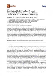
With reference to the most loaded line, Figure 12 presents the frequency temporal profiles on some of its critical stops (left hand side), and the corresponding congestion delays between successive stops (right hand side). It can be noticed that the increment of travel time between stops 4 and 5 (due both to road congestion and to boarding and alighting congestion) induces a perturbation on carrier frequencies propagating in time forward along the line. temporal profiles of frequency at consecutive stops [veh/h] stop 4

stop 5

stop 6

stop 7

12 10 8 6 4 6:00 200

line arc travel time / uncongested line arc travel time 10.0 5.0

7:00 400

12 10 8 6 4 6:00 200

7:00 400

12 10 8 6 4 6:00 200

7:00 400

12 10 8 6 4 6:00 200

7:00 400

8:00 600

8:00 600

8:00 600

8:00 600

9:00 800

9:00 800

9:00 800

9:00 800

10:00 1000

10:00 1000

10:00 1000

10:00 1000

11:00 1200

0.0 6:00 200

7:00 400

8:00 600

9:00 800

10:00 1000

11:00 1200

11:00 1200

4.0 3.0 2.0 1.0 0.0 6:00 200

7:00 400

8:00 600

9:00 800

10:00 1000

11:00 1200

11:00 1200

4.0 3.0 2.0 1.0 0.0 6:00 200

7:00 400

8:00 600

9:00 800

10:00 1000

11:00 1200

11:00 1200

4.0 3.0 2.0 1.0 0.0 6:00 200

7:00 400

8:00 600

9:00 800

10:00 1000

11:00 1200

Figure 12. line frequency propagation between different stops.

3000

inflow

available capacity

us/h 4000

A

B

outflow

C

D

2000

E

1000

6:00 6

11:00

min 10

travel time

5 0 6 6:00

us 400

11:00

queue

200 0 6 6:00

Figure 13. State evolution over time of a congested queuing arc.

11:00

28 Insert book title here Figure 13 represents the state evolution over time of a queuing arc where over saturation occurs. As long as the passenger’s inflow remains below the available capacity (interval AB), no queue is present; thus, the arc travel time is null and the outflow is equal to the inflow. When the inflow equals the available capacity a queue grows, along with the travel time, while the inflow is greater than the available capacity (interval B-C), and vice-versa decreases (interval C-D); as long as the queue is present, the outflow is equal to the available capacity. When the queue vanishes, the arc travel time returns to be null and the outflow is again equal to the inflow (interval D-E). The above numerical results confirms that the approach proposed in this work in order to solve multi mode dynamic traffic assignment is valid: in fact, all congestion effects are properly taken into account, and calculation times are reasonable also on realistic networks. However, more work is to be done in the future in order to improve the convergence of the proposed algorithm.

REFERENCES Bellei G., Gentile G., Papola N. (2003). Assegnazione alle reti multimodali in presenza di congestione. In: Metodi e Tecnologie dell’Ingegneria dei Trasporti. Seminario 2001 (G. Cantarella and F. Russo ed.s), pp. 117-134. Franco Angeli, Milano, Italy. Bellei G., Gentile G., Papola N. (2005). A within-day dynamic traffic assignment model for urban road networks. Transportation Research B 39, 1-29. Cascetta E. (2001). Transportation systems engineering: theory and methods, pp. 384-386. Kluwer Academic Publisher, UK. Crisalli U. (1999). Dynamic transit assignment algorithms for urban congested networks. In Urban Transport and the Environment for the 21st century V (L.J. Sucharov ed.), pp. 373-382. Computational Mechanics Publications. Daganzo C. F. (1997). Fundamentals of Transportation and Traffic Operations, pp. 97-112. Pergamon, Oxford, UK. DeCea J., Fernandez E. (1993). Transit assignment for congested public transport systems: an equilibrium model. Transportation Science 27, 133-147. Gentile G., Meschini L., Papola N. (2005). Macroscopic arc performance models with capacity constraints for within-day dynamic traffic assignment. Transportation Research B 39, 319-338. Gentile G., Meschini L. (2006). Fast heuristics for the continuous dynamic shortest path problem in traffic assignment. Submitted to the AIRO Winter 2005 special issue of the European Journal of Operational Research on Network Flows. Gentile G., Meschini L., Papola N. (2006). Spillback congestion in dynamic traffic assignment: a macroscopic flow model with time-varying bottlenecks. Accepted for publication in Transportation Research B.


Nguyen S., Pallottino S. (1988). Equilibrium traffic assignment for large scale transit networks. European Journal of Operational Research 37, 176-186. Nguyen S., Pallottino S., Gendreau M. (1998). Implicit Enumeration of Hyperpaths in a Logit Model for Transit Networks. Transportation Science 32, 54-64. Nguyen S., Pallottino S., Malucelli F. (2001). A modelling framework for the passenger assignment on a transport network with time-tables. Transportation Science 35, 238249. Nuzzolo A., Russo F. and Crisalli U. (2003). Transit network modelling. The schedule-based dynamic approach. Franco Angeli, Milano, Italy. Spiess H., Florian M. (1989). Optimal strategies: a new assignment model for transit networks. Transportation Research B 23, 83-102. Wu J.H., Florian M., Marcotte P. (1994). Transit equilibrium assignment: a model and solution algorithms. Transportation Science 28, 193-203. Xu, Y.W., Wu, J.H., Florian, M., Marcotte, P., Zhu, L.H. (1999). Advances in the continuous dynamic network loading problem. Transportation Science 33, 341-353.