1999: statistical methods for sensitivity and performance ... - CiteSeerX

Proceedings of the 1999 Winter Simulation Conference P. A. Farrington, H. B. Nembhard, D. T. Sturrock, and G. W. Evans, eds.

STATISTICAL METHODS FOR SENSITIVITY AND PERFORMANCE ANALYSIS IN COMPUTER EXPERIMENTS Leslie M. Moore

Bonnie K. Ray

Statistical Sciences Group, TSA-1, MS F600 Los Alamos National Laboratory Los Alamos, NM 87545-0600, U.S.A.

Dept. of Mathematical Sciences New Jersey Institute of Technology Newark, NJ 07102, U.S.A.

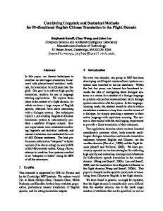
We describe statistical methods for sensitivity and performance analysis of complex computer simulation experiments. Graphical methods, such as trellis plots, are suggested for exploratory analysis of individual or aggregate performance metrics conditional on different experiment inputs. More formal statistical methods, such as analysis of variance-based methods and regression tree analysis, are used to determine variables having substantive influence on the experimental results and to investigate the structure of the underlying relationship between inputs and outputs. The methods are discussed in relation to a supply chain model of the textile manufacturing process having many possible input and output variables of interest and for a computer model used to describe the flow of material in an ecosystem.

where f represents the simulation model. If the input values are stochastic, the relationship in (1) is not exact, but contains an additional random error term, i.e., Y = f (X) + . Stochasticity may also come from within the simulation itself. However, similar methods of analysis can be applied in either case. Koehler and Owen (1996) discuss experimental design methods for computer experiments with deterministic inputs that introduce randomness by taking random input points having some particular properties. The goals of the modeling exercise may include: finding a region of X values yielding improved performance on the basis of a particular criterion for Y , sensitivity analysis of Y with respect to changes in X, finding a simple and accurate approximation of f for a particular region A of X values. For each of these goals, statistical visualization and analysis methods are applicable.

1

2

ABSTRACT

INTRODUCTION

The increasing use of computer simulation methods for modeling complex, interrelated physical or manufacturing processes has led to the need for statistical methods that can be used to understand such systems. For example, a simulation model of a manufacturing supply chain may contain many different process activities, such as receiving, processing, transporting, inspecting. Each of these activities may have many different input variables whose values can affect the resulting process performance, including the inventory replenishment strategy, manufacturing orientation, or capacity planning strategy. Outputs of interest may include, among others, measures of manufacturing cycle time, supplier lead time, total manufacturing costs, number of lost customers, and profits. In general, let X ∈ R p denote a vector of deterministic input values chosen for the simulation model and let Y ∈ R q denote the vector of output quantities. The relationship between X and Y may be denoted by Y = f (X),

STATISTICAL METHODS FOR ANALYSIS OF COMPUTER EXPERIMENTS

Both exploratory graphical methods and more formal statistical modeling techniques are useful for examining the output of computer experiments. In the following sections, we discuss the use of variance analysis for assessing input variable importance, trellis plots for graphical analysis of output with conditioning on input variables, and regression tree modeling for obtaining an approximation to f . Each of these goals relates to analysis of “input uncertainty” as opposed to uncertainty due to simulation variability. 2.1 Handling Vector Performance Measures When there are many possible performance measures associated with the simulation model, i.e., Y ∈ R q , where q > 1, the analyst may be interested not only in evaluating the effect of X on individual elements of Y , but also in evaluating the effect on a combined measure of Y , which may incorporate information concerning the importance of each performance metric relative to the overall analysis

(1)

486

Moore and Ray denotes the number of observed responses per level. As in an analysis of variance,

goal. Morrice, Butler, and Mullarkey (1998) discuss an approach to evaluating project configurations for a simulation model having multiple performance measures using multiple attribute utility functions. In this approach, vector performance measures are transformed into a scalar measure using, for example, a weighted sum of attribute utility functions for the individual measures. Other possible methods of aggregating multiple performance measures include calculation of a “desirability” function, D (Derringer and Suich, 1980), which reflects the desirable ranges for each response, yi , i = 1, · · · , q. The desirability may range from zero to one, with zero indicating least desirable and one indicating most desirable. For instance, if yi is specified to be in some target range (ai , bi ), with target value ti , then di , the desirability corresponding to yi is defined by di

=

di

=

di

=

di

=

0, yi < ai yi − ai wi [ ] , ai ≤ yi ≤ ti ti − a i yi − bi wi [ ] , ti ≤ yi ≤ bi ti − b i 0, yi > bi ,

SST O =

i

and SSA =

(4)

j

XX (yi. − y¯.. )2 , i

(5)

j

where y¯.. denotes the overall mean response and yi. denotes the mean response of the ki results at level i of the input variable A. The ratio of these two sums of squares is 2 , the estimated correlation coefficient for input variable RA A. A measure of the relative importance of input variables, taken singly, is provided in the associated R 2 values. Those variables having large R 2 values are deemed to be most important in affecting the output of the model. These variables are analogous to significant ”main effects” in an ANOVA framework (Box and Draper, 1987). Assuming that sufficient experimental runs of the model exist, the technique is easily extended to assess the impact of two or more input variables simultaneously. Alternatively, the procedure can be used in a sequential manner, i.e., incremental correlation ratios can be computed for a second input variable, given the effect of each important main effect input variable. See McKay, Morrison, and Upton (1998). A recent paper by McKay, Fitzgerald, and Beckman (1999) studies the effect of the assumed number of levels for an input variable, l, and the sample size, ki , per level on the discriminating ability of R 2 in determining important inputs. In McKay, Fitzgerald, and Beckman (1999), “replicated” Latin hypercube samples form the basis of the experiment design. Orthogonal arrays have also been suggested for the design of experiments for computer models in Koehler and Owen (1996) and Owen (1992). The technique can be extended to the case of p-variate responses by considering a function of SSA(SST O)−1 , where SSA and SST O are p×p matrices, and an appropriate function may be the determinant function. This is analogous to test statistics used in multivariate ANOVA applications to assess main and interaction effects (Box and Draper, 1987).

(2)

where wi denotes a weight that can be chosen to give more (wi > 1) or less (wi < 1) weight to the goal. The overall desirability function is defined by q Y P1 D = ( diri ) ri ,

XX (yij − y¯.. )2 ,

(3)

i=1

where ri is a value between one and five reflecting the relative importance of response yi . For certain statistical methods, techniques have been developed to handle vector response variables explicitly. However, unless otherwise stated, we assume that the referenced response variable in the following discussions is scalar. 2.2 Variance Analysis McKay et al. (1992) suggests the conditional variance of the output as a meaningful measure of importance in identifying inputs having significant impact on the simulation results. Analogous to analysis of variance (ANOVA), output variability is decomposed into components that can each be attributable to an input variable of interest; these quantities are then compared to the total variability. This method has been used, for example, by McKay, Morrison, and Upton (1998) for evaluating prediction uncertainty in simulation models. For a particular input variable, A, denote associated responses by yij , i = 1, . . . , l, j = 1, . . . , ki , where l denotes the number of levels of the input of interest and ki

2.3 Graphical Analysis Once a subset of important inputs is selected, it is desirable to look in more detail at how Y changes in response to changes in these inputs. Trellis graphs (Becker, Cleveland, and Shyu, 1996), which allow the analyst to view relationships between different variables under fixed conditions of other variables, are useful at this stage. Suppose you have a data set based on multiple variables and you would like to see how plots of two variables change

487

Statistical Methods for Sensitivity and Performance Analysis in Computer Experiments equilibrium. The flow between compartments is modeled by a system of differential equations, where the inputs X to the system are a set of 84 equation “transfer coefficients”, each assumed to have a Beta distribution with (possibly) different range. The range of each variable was divided into fourteen intervals, and each input was identified with fourteen discretized values as levels. An experiment was designed to investigate R 2 values for the 84 factors individually and for all (3570) pairs of the 84 factors. The experiment design was generated from a highly fractionated factorial design for 84 factors with 83 levels. Simple fractional factorial designs for two or three level factors are described in most statistics textbooks on experiment design including Box, Hunter and Hunter (1978). Addelman and Kempthorne (1961) describe maineffect factorial design plans and orthogonal arrays. The fraction used here is a Resolution III design in 832 = 6889 runs which is also an orthogonal array of strength two. The Resolution III and strength two properties indicate a balance such that every pair of levels associated with two factors occurs once. By further "collapsing" the 83 levels of a given factor to fourteen levels by a natural mapping of six values to one with the fourteenth level being assigned from values 79 to 83, the design is assured of having about 25 to 36 samples associated with each of pair of levels associated with two factors. This process of collapsing factor levels does not ensure that the resulting runs are distinct. When duplicated runs are eliminated, the experiment design has 6820 runs. Figure 1 shows a plot of the R 2 values for each input variable, sorted from largest to smallest, with the ten most ”important” input variables identified. Figure 2 shows a similar plot of R 2 values corresponding to two-way interactions between pairs of input variables. Important factors are identified with larger R 2 values, and as the curves formed by the plots illustrated in Figures 1 and 2 level off, the associated factors are not considered important. Thus, for the current study, we might restrict attention to 5-10 factors (or pairs) for further study. Figure 3 shows a regression tree for the environmental pathways model based on the top ten input variables selected in the R 2 analysis. The values at each terminal node represent the average concentration for the associated region of the input variables. The regression tree analysis is a feature of Splus (MathSoft 1998). The partitioning of the range of levels of a factor is not indicated on the display in Figure 3, but is available in the Splus output. Following the right branch of the tree all the way down to its terminal node, we have that when input variable 69 has level {1, 10, 11, 12, 13, 14, 2, 3, 4, 7, 8, 9}, variable 68 has level {4, 5, 6}, variable 84 has level {3, 4, 5, 12, 13}, variable 24 has level {1, 8} and variable 1 has level {12, 6}, the average concentration is 13.0. Thus a region of the input predictor space giving “extreme” values of Y is easily

with variations in a third "conditioning" variable. Trellis graphics, as implemented in Splus 4.0 and higher (MathSoft, 1998), can be used to view the output data in a series of panels, where each panel contains a subset of the original data divided into intervals of the conditioning variable(s). In this way, interaction effects between input variables can be assessed graphically. Trellis graphics are quite general, in that most types of plots can be accommodated in the conditioning framework. Factor interaction plots of the type commonly used in ANOVA can also graphically show the effect of one factor at different levels of a second factor, but are not very useful for examining higher-level interactions. 2.4 Regression Trees Tree-based modeling is an exploratory technique for uncovering structure in data, which can be used for, among other things, screening variables and summarizing large multivariate datasets. For a numeric scalar response Y , an example of a regression rule for description or prediction is: if xi > t and xj ∈ {1, 2}, then the predicted value of Y is c, where t and c are real values and {1, 2} denote levels of categorical input variable xj . A regression tree is the collection of many such rules displayed in the form of a binary tree. The rules are determined by a procedure known as recursive partitioning. The model is simply a set of partitions of the input variable space such that values of Y are relatively constant in that partition. The predicted value of Y for a particular region is just the sample average of the responses corresponding to values of the input variables which fall in that region. Tree-based models are adept at capturing non-additive and general interactions between input variables, which is almost always the case in complex simulation models. Breiman et al. (1984) gives a detailed discussion of classification and regression tree methodology. Extensions to the regression tree methodology such as treed regression, which fits linear regression models in each region, have also been discussed in the literature (Alexander and Grimshaw, 1996). For treed regressions, it is conceivable that the response Y may be vector-valued, as in the standard linear multivariate regression framework, although, to the best of our knowledge, this has not been discussed in the literature. In the following section, we apply some of the discussed techniques to two examples. 3

APPLICATIONS

Our first example is for a compartmental model used to describe the flow of material in an ecosystem. The model calculates concentrations in 15 subsystems, or compartments, as functions of time. One output of particular interest is the concentration, Y , in one of the compartments at system

488

Moore and Ray R2 Values for Input Variable Main Effects Regression Tree for Environmental Pathways Model 69

0.05

V69 | V68 V68 V2 V63V1 V46 V84 V1 V69 V84 V63 0.053 0.3 0.031 0.09 V24 V2 0.091 0.30.88 1.9 0.0870.43 0.18 2.3 1.3 1.8 V63 V2 V35 0.2 0.063 0.19 1.5 V63

Top Ten Variables: {1,2,24,35,46,63,67,68,69,84}

V84

0.03

24 2

Right-most Tree path

0.02

R2

0.04

68

V24 0.260

V69:1,10,11,12,13,14,2,3,4,7,8,9 V68:4,5,6

0.01

V84:12,13,3,4,5 V24:1,8 V1:12,6

V46

V1

0.00

V24 V63 6.4 0.461.8 3.5 0

20

40 Rank

60

4.8 13.0

80

Figure 1: Ranked R 2 Values for Main Effects of Input Variables to Environmental Pathways Compartmental Model

Figure 3: Regression Tree for Concentration as a Function of Top Ten Input Variables for Environmental Pathways Compartmental Model

R2 Values for Two-way Interactions (2,68)

0.25 0.20

(68,69)

0.10

0.15

R2

algorithms, marketing strategy, cost trade-offs, inventory replenishment strategy, manufacturing orientation, capacity planning strategy, or scheduling techniques. It is anticipated that, across sectors, up to sixty activities might be modeled dynamically in the simulation under development. This suggests possibly designing experiments with hundreds of input variables and analyzing process performance on the basis of between five and ten output variables. However, the prototype study was limited to a few inputs, namely forecast method and manufacturing orientation. In particular, available simulation output was based on only four manufacturing orientations: “as is” push, “to be” push, “to be” pull, and “to be” synchronous flow. Additionally, the pilot study included only parts of three sectors: textile, apparel and retail. Output variables of interest included process throughput, cycle time, supplier lead time, and inventory turnover. Figure 4 shows trellis plots of the supplier lead times for 432 days (in hours) for each of the four manufacturing strategies and each of three receiving activities in the supply chain. In the plot, R6 denotes the first receiving activity (in the textile sector), while R13 and R18 denote receiving activities that occur in the apparel sector. Similar plots can be constructed for activities aggregated across a sector, or for supplier lead time at different time scales (monthly, quarterly), etc. Up to four conditioning variables can be used to construct the trellis display. For the supply chain model under development, we anticipate that trellis graphics will be useful for considering the effects of such things as inventory replenishment strategies under different manufacturing orientations for different sectors of the textile manufacturing process.

(2,67) (2,65)

0

100

200

300

400

500

Rank

Figure 2: Ranked R 2 Values for Two-Way Interactions Between Input Variables to Environmental Pathways Compartmental Model identified. The first input variable that is partitioned is 69, which also had the largest R 2 value for main effects. Our second example is a simulation model of a textile manufacturing supply chain which is currently in development at Los Alamos National Laboratory. A prototype simulation was developed to study the supply chain production of a nylon jacket and is reported in Chandra, Nastasi, Powell and Ostic (1996). The textile manufacturing process consists of four sectors: fiber, textiles, apparel, and retail. For a particular product, several companies may be represented in each sector, with potentially many processes within a company, and many activities within a process. For every activity, up to a dozen input variables may be required which determine such things as demand forecast

489

Statistical Methods for Sensitivity and Performance Analysis in Computer Experiments

1

Becker, R.A., J.M. Chambers, and A.R. Wilks. 1988. The New S Language: A Programming Environment for Data Analysis and Graphics. New York: Chapman and Hall. Becker, R.A., W.S. Cleveland, and M.-J. Shyu. 1996. The visual design and control of trellis display. Journal of Computational and Graphical Statistics 5:123-155. Box, G.E.P. and N.R. Draper. 1987. Empirical modelbuilding and response surfaces. Wiley Series in Probability and Mathematical Statistics: Applied Probability and Statistics. New York: John Wiley & Sons, Inc. Box, G. E. P., W. G. Hunter, and J. S. Hunter. 1978. Statistics for experiments: An introduction to design, data analysis, and model building. Wiley Series in Probability and Mathematical Statistics. New YorkChichester-Brisbane: John Wiley & Sons. Breiman L., J.H. Friedman, R.A. Olshen, and C.J. Stone. 1984. Classification and Regression Trees. Belmont, CA: Wadsworth International Group. Chandra, C. A. Nastasi, D. Powell, and J. Ostic. 1996. Enterprise simulation analysis of the nylon jacket pipeline. Technical Report LA-UR-97-154, Los Alamos National Laboratory. Derringer, G. and R. Suich. 1980. Simultaneous optimization of several response variables. Journal of Quality Technology, 12:214-219. Koehler, J. R. and A. B. Owen. 1996. Computer experiments. Design and analysis of experiments. Handbook of Statistics, 13:261–308, Amsterdam:North-Holland. Law, A.M. and W.D. Kelton. 1991. Simulation modeling and analysis, 2nd ed. New York:McGraw-Hill. McKay, M.D., R.J. Beckman, L.M. Moore, and R. R. Picard. 1992. An alternative view of sensitivity in the analysis of computer codes. In Proceedings of the Section on Physical and Engineering Sciences of the American Statistical Association, 87-92. McKay, M.D., J.D. Morrison, and S. Upton. 1998. Evaluating prediction uncertainty in simulation models. Technical Report LA-UR-98-1362, Los Alamos National Laboratory (to appear in Computer Physics Communications). McKay, M.D., M.A. Fitzgerald, and R.J. Beckman. 1999. Sample size effects when using R 2 to measure model importance. Unpublished manuscript, Los Alamos National Laboratory. Morrice, D. J., J. Butler, and P. W. Mullarkey. 1998. An approach to ranking and selection for multiple performance measures. In Proceedings of the 1998 Winter Simulation Conference, ed. D.J. Medeiros, E.F. Watson, J.S. Carson, and M.S. Manivannan, 719-725. Institute of Electrical and Electronics Engineers, Piscataway, NJ.

1

R13 SLTh.AIP

R13 SLTh.TBP

R13 SLTh.TBPl

R13 SLTh.TBS

R18 SLTh.AIP

R18 SLTh.TBP

R18 SLTh.TBPl

R18 SLTh.TBS

1000

SLTh

400

1000 400 R6 SLTh.AIP

R6 SLTh.TBP

R6 SLTh.TBPl

R6 SLTh.TBS

1000 400

1

1 supplier.lth\0

Figure 4: Trellis Time Series Plots of Supplier Lead Times for Receiving Activities

4

CONCLUSIONS

We have presented several statistical techniques that can be used to investigate sensitivity and performance analysis of simulation models. Although the specific examples discussed in this paper pertain to a deterministic computer model and a finite-horizon supply chain simulation with deterministic inputs, the techniques can be also be applied to steady-state simulations using the method of batch means to obtain approximately independent observations of performance measures (see, for example, Law and Kelton, 1991). Future work will focus on applying these techniques in a more thorough investigation of the manufacturing supply chain model discussed in Section 3. In particular, we plan to implement an appropriate experimental design and apply the multivariate methods mentioned in Section 2 to assess the supply chain performance across different activities and time horizons. ACKNOWLEDGEMENTS The authors thank T.S.A. Juan of Los Alamos National Laboratory for helpful discussions and ideas. REFERENCES Addelman, S. and O. Kempthorne. 1962. Some maineffect plans and orthogonal arrays of strength two. The Annals of Mathematical Statistics, 32:1167-1176. Alexander, W.P. and S.D. Grimshaw. 1996. Treed regression. Journal of Computational and Graphical Statistics 5:156-175.

490

Moore and Ray Owen, A. B. 1992. Orthogonal arrays for computer experiments, integration and visualization. Statistica Sinica, 2:439-452. Splus 4.5 Guide to Statistics. 1998. Data Analysis Division, Mathsoft, Seattle. AUTHOR BIOGRAPHIES

LESLIE M. MOORE is a Technical Staff Member in the Statistical Sciences Group at Los Alamos National Laboratory. She holds a B.S. in Mathematics and a Ph.D. in Mathematics, concentration in Statistics, from the University of Texas at Austin. Her research interests include experiment design, including the design and analysis of computer experiments, generalized linear mixed models, and statistical intervals. BONNIE K. RAY is an Associate Professor in the Dept. of Mathematical Sciences at the New Jersey Institute of Technology and is currently a research affiliate with the Statistical Sciences group at Los Alamos National Laboratory. She holds a Ph.D. in Statistics from Columbia University and a B.S. in Mathematics from Baylor University. Her research interests include time series analysis, statistical computing, and statistical graphics.

491