Current and Potential Statistical Methods for Monitoring ... - CiteSeerX

Current and Potential Statistical Methods for Monitoring Multiple Data Streams for Bio-Surveillance Galit Shmueli and Stephen E. Fienberg June 9, 2005

2

0.1

Introduction

A recent review of the literature on surveillance systems revealed an enormous number of researchrelated articles, a host of websites, and a relatively small (but rapidly increasing) number of actual surveillance systems, especially for the early detection of a bioterrorist attack [Bravata et al., 2004]. Modern bio-terrorism surveillance systems such as those deployed in New York City, Western Pennsylvania, Atlanta, and Washington, DC routinely collect data from multiple sources, both traditional and non-traditional, with the dual goal of the rapid detection of localized bio-terrorist attacks and related infectious diseases. There is an intuitive notion underlying such detection systems, namely that detecting an outbreak early enough would enable public health and medical systems to react in a timely fashion and thus save many lives. Demonstrating the real efficacy of such systems, however, remains a challenge that has yet to be met, and several authors and analysts have questioned their value, e.g., see [Reingold, 2003, Stoto et al., 2004, Stoto et al., 2005]. This article explores the potential and initial evidence adduced in support of such systems and describes some of what seems to be emerging as relevant statistical methodology to be employed in them. Public health and medical data sources include mortality rates, lab results, emergency room visits, school absences, veterinary reports and 911 calls. Such data are directly related to the treatment and diagnosis that would follow a bio-terrorist attack. They might not, however, detect the outbreak sufficiently fast. Several recent national efforts have been focused on monitoring “earlier” data sources for the detection of bio-terrorist attacks or other outbreaks, such as over-the-counter (OTC) medication sales, nurse hotlines, or even searches on medical websites (e.g., WebMD). This assumes that people, who are not aware of the outbreak and are feeling sick, would generally seek self-treatment before approaching the medical system and that an outbreak signature will manifest itself earlier in such data. According to [Wagner et al., 2003], preliminary studies suggest that sales of OTC health care products can be used for the early detection of outbreaks, but research progress has been slow due to the difficulty that investigators have has in acquiring suitable data to test this hypothesis for sizeable outbreaks. Some data of this sort are already being collected (e.g., pharmacy and grocery sales). Other potential nontraditional data sources that are currently not-collected (e.g. browsing in medical websites; automatic body sensor devices), could contain even earlier signatures of an outbreak.1 To achieve rapid detection there are several requirements that a surveillance system must satisfy: frequent data collection, fast data transfer (electronic reporting), real-time analysis of incoming data, and immediate reporting. Since the goal is to detect a large localized bio-terrorist attack, the collected information must be local, but sufficiently large to contain a detectable signal. And, of course, the different sources must carry an early signal of the attack. There are, however, tradeoffs between these features: although we require frequent data for rapid detection, too frequent data might be too noisy to the degree that the signal is too weak for detection. A typical solution for too-frequent data is temporal aggregation. Two examples where aggregation is used for bio-surveillance are aggregating over-thecounter medication sales from hourly to daily counts ([Goldenberg et al., 2002]), and aggregating daily hospital visits into multi-day counts ([Reis et al., 2003]). A similar tradeoff occurs between the level of localization of the data and their amount. If the data are too localized, there might be insufficient data for detection, whereas spatial aggregation might dampen the signal. Another important set of considerations that limit the frequency and locality of collected data relate to confidentiality and data disclosure issues (concerns over ownership, agreements with retailers, personal and organizational privacy, etc.) Finding a level of aggregation that contains a strong enough signal, that is readily available for collection without confronting legal obstacles, and yet is sufficiently rapid and localized for rapid detection is clearly a challenge. We describe some of the confidentiality and privacy issues briefly here. There are many additional challenges associated with the phases of data collection, storage, and transfer. These include standardization, quality control, confidentiality, etc. (see [Fienberg and Shmueli, 2004]). In this paper we focus on the statistical challenges associated with the data monitoring phase, and in particular, data in the form of multiple time series. We start by describing 1 While our focus in this article is on passive data collection systems for syndromic surveillance, there are other active approaches that have been suggested, e.g., screening of blood donors [Kaplan et al., 2003], as well as more technological fixes, such as biosensors [Sullivan, 2003] and “Zebra” chips for clinical medical diagnostic recording, data analysis, and transmission [Casman, 2004].

0.2. Types of Data Collected in Surveillance Systems

3

data sources that are collected by some major surveillance systems and their characteristics. We then examine various traditional monitoring tools and approaches that have been in use in statistics in general, and in bio-surveillance in particular. We discuss their assumptions and evaluate their strengths and weaknesses in the context of bio-surveillance. The evaluation criteria are based on the requirements of an automated, nearly real-time surveillance system that performs online (or prospective) monitoring of incoming data. These are clearly different than for retrospective analysis ([Sonesson and Bock, 2003]), and include computational complexity, ease of interpretation, roll-forward features, and flexibility for different types of data and outbreaks. Currently, the most advanced surveillance systems routinely collect data from multiple sources on multiple data streams. Most of the actual statistical monitoring, however, is typically done at the univariate time series level, using a wide array of statistical prediction methodologies. Ideally, multivariate methods should be used so that the data can be treated in an integrated way, accounting for the relationships between the data sources. We describe the traditional statistical methods for multivariate monitoring and their shortcomings in the context of bio-surveillance. Finally, we describe monitoring methods, in both the univariate and multivariate sections, that have evolved in other fields and appear potentially useful for bio-surveillance of traditional and non-traditional temporal data. We describe the methods and describe their strengths and weaknesses for modern bio-surveillance.

0.2

Types of Data Collected in Surveillance Systems

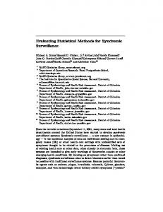
Several surveillance systems aimed at rapid detection of disease outbreaks and bio-terror attacks have been deployed across the USA in the last few years, including the Realtime Outbreak and Disease Surveillance system (RODS) and National Retail Data Monitor (NRDM) in Western Pennsylvania, the Early Notification of Community-based Epidemics system (ESSENCE) in the Washington DC area (which also monitors many Army, Navy, Air Force, and Coast Guard data worldwide), the New York City Department of Health and Mental Hygiene (NYC-DOHMH) system, and recently the BioSense system by the Centers for Disease Control and Prevention. Each system collects information on multiple data sources with the intent of increasing the certainty of a true alarm by verifying anomalies found in various data sources ([Pavlin et al., 2003]). All of these systems collect data from medical facilities, usually at a daily frequency. These include emergency rooms admissions (RODS, NYC), visits to military treatment facilities (ESSENCE), and 911 calls (NYC). Non-traditional data include over-the-counter medication and health-care product sales at grocery stores and pharmacies (NRDM, NYC, ESSENCE), prescription medication sales (ESSENCE), HMO billing data (ESSENCE), and school/work absenteeism records (ESSENCE). We can think of the data in a hierarchical structure: the first level consists of the data source (e.g., ER or pharmacy), and then within each data source there might be multiple time series, as illustrated in figure 1. This structure suggests that series that come from the same source should be more similar to each other than to series from different sources. This can influence the type of monitoring methods used within a source as opposed to methods for monitoring the entire system. For instance, within-source series will tend to share variation sources such as holidays, closing dates, and seasonal effects. Pharmacy holiday closing hours will influence all medication categories equally but not school absences. From a modelling point of view this structure raises the question whether a hierarchical model is needed or else all series can be monitored using a flat multivariate model. In practice, most traditional multivariate monitoring schemes and a wide range of applications consider similar data streams. Very flexible methods are needed in order to integrate all the data within a system that is automatic, computationally efficient, timely, and with low false alarms. In the following sections we describe univariate and multivariate methods that are currently used or can potentially be used for monitoring the various multiple data streams. We organize and group the different methods by their original or main field of application, and discuss their assumptions, strengths, and limitations in the context of bio-surveillance data.

0.3

Monitoring Univariate Data Streams

The methods used in bio-surveillance borrow from several fields, with statistical process control being the most influential. Methods from other fields have also been used occasionally, with most relying on

4

Data Source

Information collected

Respiratory ER admissions (ICD-9 codes)

Cough Viral infection

Analgesics Over-the-counter medication sales

Cough relief Nasal decongentant Allergy treatment

School absence

Nurse hotlines

Figure 1. Sketch of data hierarchy: each data source can contain multiple time series traditional statistical methods such as regression and time series models. Although different methods might be more suitable for different data streams or sources, there are advantages to using a small set of methods for all data streams within a single surveillance system. This simplifies automation, interpretability, and coherence, and the ability to integrate results from multiple univariate outputs. The principle of parsimony, which balances performance and simplicity, should be the guideline. We start by evaluating some of the commonly used monitoring methods and then describe other methods that have evolved or have been applied in other fields, which are potentially useful for biosurveillance.

0.3.1

Current Common Approaches

Statistical Process Control Monitoring is central to the field of statistical process control. Deming, Shewhart, and others revolutionized the field by introducing the need and tools for monitoring a process in order to detect abnormalities at the early stages of production. Since the 1920’s the use of control charts has permeated into many other fields including the service industry. One of the central tools for process control is the control chart, which is used for monitoring a parameter of a distribution. In its simplest form the chart consists of a centerline, which reflects the target of the monitored parameter, and control limits. A statistic is computed from an iid sample every time point, and its value is plotted on the chart. If it exceeds the control limits, the chart flags an alarm, indicating a change in the monitored parameter. Statistical methods for monitoring univariate and multivariate time series tend to be model-based. The most widely used control charts are Shewhart charts, Moving Average charts, and cumulative sum (CuSum)

0.3. Monitoring Univariate Data Streams

5

charts. Each of these methods specializes in detecting a particular type of change in the monitored parameter ([Box and Luceo, 1997]). We now briefly describe the different charts. Let yt be a random sample of measurements taken at time t (t = 1, 2, 3 . . .). In a Shewhart chart the monitoring statistic at time t, denoted by St , is a function of yt : (1) St = f (yt ) The statistic of choice depends on the parameter that is monitored. For instance, if the process mean is monitored, then the sample mean (f (yt ) = y t ) is used. If the process variation is monitored, a popular choice is the sample standard deviation (f (yt ) = st ). The monitoring statistic is drawn on a time plot, with lower and upper control limits. When a new sample is taken, the point is plotted on the chart, and if it exceeds the control limits it raises an alarm. The assumption behind the classic Shewhart chart is that the monitoring statistic follows a normal distribution. This is reasonable when the sample size is large enough relative to the skewness of the distribution of yt . Based on this assumption, the control limits are commonly selected as ±3 standard deviations of the monitoring statistic (e.g., if the √ sample mean is the monitoring statistic then the control limits are ±3σ/ n) in order to achieve a low false alarm rate of 2φ(−3) = 0.0027. Of course, the control limits can be chosen differently to achieve a different false alarm rate. If the sample size at each time point is n = 1, then we must assume that yt are normally distributed for the chart to yield valid results. Alternatively, if the distribution of f (yt ) (or yt ) is known then a valid Shewhart chart can be constructed by choosing the appropriate percentiles of that distribution for the control limits, as discussed in [Stoto et al., 2005]. Shewhart charts are very popular because of their simplicity. They are very efficient at detecting moderate to large spike-type changes in the monitored parameter. Since they do not have a “memory”, a large spike is immediately detected by exceeding the control limits. However, Shewhart charts are not useful for detecting small spikes or longer-term changes. In those instances we need to retain a longer “memory”. One solution is to use the “Western Electric” rules. These rules raise an alarm when a few points in a row are too close to a control limit, even if they do not exceed it. Although such rules are popular and imbedded in many software programs, their addition improves detection of real abberations at the cost of increased false alarms. The tradeoff turns out to be between the expected time-to-signal and its variability ([Shmueli and Cohen, 2003]). An alternative is to use statistics that have longer memories. Three such statistics are the moving average (MA), the exponentially weighted moving average (EWMA), and the cumulative sum (CuSum). Moving average charts use a statistic that relies on a constant-size window of the k last observations: M At =

k X

f (yt−j+1 )/k

(2)

j=1

Pk The most popular statistic is a grand mean ( j=1 y t−j+1 /k). These charts are most efficient for detecting a step increase/decrease that lasts k time Ptpoints. The original CuSum statistic defined by σ1 i=1 (yt − µ) keeps track of all the data until time t ([Hawkins and Olwell, 1998]). However, charts based on this statistic are awkward graphically. A widely used adaptation is the tabular CuSum which restarts the statistic whenever it exceeds zero. The one-sided tabular CuSum for detecting an increase is defined as CuSumt = max{0, (yt∗ − k) + CuSumt−1 }

(3)

where yt∗ = (yt − µ)/σ are the standardized observations, and k is proportional to the size of the abnormality that we want to detect. This is the most efficient statistic for detecting a step change in the monitored parameter. However, it is less useful for detecting a spike since it would be masked by the long memory. In general, time series methods that place heavier weight on recent values are more suitable for short-term forecasts ([Armstrong, 2001]). The EWMA statistic is similar to the CuSum, except that it weights the observations as a function of their recency, with recent observations taking the highest weight: EW M At = αyt + (1 − α)EW M At−1

t−1 X =α (1 − α)j f (yt−j ) + (1 − α)EW M A0 j=0

(4)

6 where 0 < α ≤ 1 is the smoothing constant ([Montgomery, 2001]). This statistic is best at detecting an exponential increase in the monitored parameter. It is also directly related to exponential smoothing methods (see below). For further details on these methods see [Montgomery, 2001]. In bio-surveillance, the EWMA chart was used for monitoring weekly sales of over-the-counter electrolytes to detect pediatric respiratory and diarrheal outbreaks ([Hogan et al., 2003]), and is used in ESSENCE II to monitor ER admissions in small geographic regions ([Burkom, 2003b]). Since the statistic in these last three cases is a weighted average/sum over time, the normality assumption of yt is less crucial for adequate performance due to the central limit theorem, especially in the case of the EWMA ([Reynolds and Stoumbos, 2004, Arts et al., 2004]). The main disadvantage of all these monitoring tools is that they assume statistical independence of the observations. Their original and most popular use is in industrial process control where samples are taken from the production line at regular intervals, and a statistic based on these assumably independent samples is computed and drawn on the control chart. The iid assumption is made in most industrial applications, whether correct or not. Sometimes the time between samples in increased in order to minimize correlation between close samples. In comparison, the types of data collected for bio-surveillance are usually time series that are collected on a frequent basis in order to achieve timeliness of detection, and therefore autocorrelation is inherent. For such dependent data streams the use of distribution-based or distribution-free control charts can be misleading is the direction of increased false alarm rates ([Montgomery, 2001], p. 375). A common approach to dealing with autocorrelated measurements is to approximate them using a time series model and monitor the residual error using a control chart ([Ganesan et al., 2004]). The assumption is that the model accounts for the dependence and therefore the residuals should be nearly independent. Such residuals will almost never be completely independent, however, and the use of control charts to monitor them should be done cautiously. This is where time series analysis emerges in anomaly detection applications in general, and in bio-surveillance in particular. Moreover, because the forecast at every time point is used to “test” for anomalies, we need to deal with the multiple testing problem for dependent tests, and possibly use variations on the new literature on False Discovery Rates (FDR) to control familywise type I errors [Benjamini and Hochberg, 1995, Efron et al., 2001]. Time Series Methods The most well-known class of time series models used by statisticians are Autoregressive-MovingAverage (ARMA) models. Conceptually they are similar to regressing the current observations on a window of previous observations while assuming a particular auto-covariance structure. An ARMA(p,q) model is defined as q p X X θj ²t−j (5) αi yt−i + ²t − yt = µ + i=1

j=1

where αi and θj are parameters and ²t−q . . . ²t are white noise (having mean 0 and standard deviation σ² ). In order to fit an ARMA model the modeler must determine the order of the autoregression p, and the order of the moving-average component, q. This task is not straightforward and requires experience and expertise (for example, not every selection of p and q yields a causal model). After p and q are determined there are p + q + 1 parameters to estimate, usually through non-linear least squares and conditional maximum likelihood. The process of selecting p and q and estimating the parameters is cyclical [Box et al., 1994] and typically takes several cycles until a satisfactory model is found. There do exist some software packages that have automated procedures for determining p and q and estimating those parameters. ARMA models can combine external information by adding predictors in the model. This allows to control for particular time points that are known to have a different mean by adding indicators with those time points. Such modifications are especially useful in the bio-surveillance context, since effects such as weekend/weekday and holidays are normally present in medical and non-traditional data. ESSENCE II, for instance, uses an autoregressive model that controls for weekends, holidays, and post-holidays through predictors ([Burkom, 2003b]). ARMA models assume that the series is stationary over time (i.e., the mean, variance, and autocovariance of the series remains constant throughout the period of interest). In practice, fitting of an ARMA model to data usually requires an initial pre-processing step where the data are transformed in

0.3. Monitoring Univariate Data Streams

7

one or more ways until a stationary or approximately stationary series emerges. The most popular generalization of ARMA models for handling seasonality and trends is to add a differencing transformation, thereby yielding an autoregressive-integrated-moving-average (ARIMA) model of the form: (1 − α1 B − α2 B 2 − . . . − αp B p )[(1 − B)d (1 − Bs)D yt − µ] = (1 − θ1 B − . . . − θq B q )²t ,

(6)

where B is the back-shift operator (Byt = yt−1 ), d > 0 is the degree of non-seasonal differencing, D > 0 is the degree of seasonal differencing, and s is the length of a seasonal cycle. Determining the level of differencing is not trivial, and over- and under-differencing can lead to problems in modelling and forecasting [Crato and Ray, 1996]. Although this model allows flexibility, in practice the model identification step is complicated and highly data specific, and requires expertise of the modeler. Another disadvantage of ARIMA models is their computational complexity. With thousands of observations, the method requires considerable computer time and memory ([SAS, 2004b]). To summarize, the common statistical approach towards monitoring has been mostly distribution based. Recent advances in data availability and collection in the process industry have led authors such as [Willemain and Runger, 1996] to emphasize the importance of model-free methods. It appears, though, that such methods have already evolved and have been used in other fields! Next, we describe a few such methods that are distribution-free.

0.3.2

Monitoring Approaches in Other Fields

Monitoring methods have been developed and used in other fields such as machine learning, computer science, geophysics, and chemical engineering. Also forecasting, which is related to monitoring, has had advances in fields such as finance and economics. In these fields there exist a wealth of very frequent autocorrelated data, the goal is the rapid detection of abnormalities (“anomaly detection”) or forecasting, and the developed algorithms are flexible and computationally efficient. We describe a few of the methods used in these fields and evaluate their usefulness for bio-surveillance. Anomaly detection in machine learning emphasizes automated and usually model-free algorithms that are designed to detect local abnormalities. Even within the class of model-free algorithms, there is a continuum between those that are intended to be completely “user-independent” and those that require expert knowledge integration by the user. An example for the former is the Symbolic Aggregate approXimation (SAX), which is a symbolic representation for time series that allows for dimensionality reduction and indexing ([Lin et al., 2003]). According to its creators, “anomaly detection algorithms should have as few parameters as possible, ideally none. A parameter free algorithm would prevent us from imposing our prejudices, expectations, and presumptions on the problem at hand, and would let the data itself speak to us” ([Keogh et al., 2004]). In bio-surveillance there exists expert knowledge about the progress of a disease, its manifestation in medical and public health data, etc. An optimal method would then be distribution-free and parsimonious, but would allow the integration of expert knowledge in a simple way. Exponential Smoothing Exponential smoothing (ES) is a class of methods that is very widely used in practice (e.g., for production planning, inventory control, and marketing ([Pfeffermann and Allon, 1989])) but not so in the bio-surveillance field. ES has gained popularity mostly because of its usefulness as a short-term forecasting tool. Empirical research by [Makridakis et al., 1982] has shown simple exponential smoothing (SES) to be the best choice for one-step-ahead forecasting, from among 24 other time series methods and using a variety of accuracy measures. Although the goal in bio-surveillance is not forecasting, ES methods are relevant because they can be formulated as models ([Chatfield et al., 2001]). Non-traditional bio surveillance data include economic series such as sales of medications, health-care products, and grocery items. Since trends, cycles, and seasonality are normally present in sales data, more advanced ES models have been developed to accommodate non-stationary time series with additive multiplicative seasonality and/or linear/exponential/dampened trend components. A general formulation of an ES model assumes that the series is comprised of a level, trend (the change in level from last period), seasonality (with M seasons), and error. To illustrate the model formulation, estimation, and forecasting

8 Exponential smoothing method Simple exponential smoothing Holt’s (double) linear trend method Damped-trend linear method Additive Holt-Winter’s (triple) method Multiplicative Holt-Winter’s (triple) method

ARIMA/SARIMA equivalent ARIMA(0,1,1) ARIMA(0,2,2) ARIMA(1,1,2) SARIMA(0,1,p+1)(0,1,0)p [Koehler et al., 2001]’s dynamic nonlinear state-space mode

Table 1. The equivalence between some exponential smoothing and (Seasonal)-ARIMA models. The notation ARIM A(p, d, q)(P, D, Q)s corresponds to an ARIMA(p,d,q) with seasonal cycle of length s, P -order autoregressive seasonality, seasonal differencing of order D, and seasonal moving average of order Q.

processes, consider an additive model of the form: yt = local mean + seasonal factor + error

(7)

where the local mean is assumed to have an additive trend term and the error is assumed to have zero mean and constant variance. At each time t, the smoothing model estimates these time-varying components with level, trend, and seasonal smoothing states denoted by Lt , Tt , and St−i (i = 0, . . . , M − 1), respecitively2 . The smoothing process starts with an initial estimate of the smoothing state, which is subsequently updated for each observation using the updating equations: Lt+1 = α(yt+1 − St+1−M ) + (1 − α)(Lt + Tt ) Tt+1 = β(Lt+1 − Lt ) + (1 − β)Tt St+1 = γ(yt+1 − Lt+1 ) + (1 − γ)St+1−M (8) where α, β and γ are the smoothing constants. The m-step-ahead forecast at time t is yˆt+m = Lt + mTt + St+m−M

(9)

A multiplicative model of the form Yt = (Lt−1 + tTt−1 )St−i ²t can be obtained by applying the updating equations in (8) to log(yt ). The initial values L0 , T0 , and the M seasonal components at time 0 can be estimated from the data using a centered moving average (see [Pfeffermann and Allon, 1989] and [NIS, 2004] for details). The three smoothing constants are either determined by expert knowledge, or estimated from the data by maximizing a well-defined loss function (e.g., mean of squared one-stepahead forecast errors). From a modelling point of view, many ES methods have ARIMA, SARIMA, and structural models equivalents, and they even include a class of dynamic non-linear state space models that allow for changing variance ([Chatfield et al., 2001]). Table 1 summarizes some of these equivalences. It is noteworthy that some of the SARIMA equivalents are so complicated that they are most unlikely to be identified in practice ([Chatfield et al., 2001]). Furthermore, [Chatfield et al., 2001] show that there are multiple generating processes for which a particular ES method is optimal in the sense of forecast accuracy, which explains their robust nature. The advantage of these models is their simplicity of implementation and interpretation, their flexibility for handling many types of series, and their suitability for automation ([Chatfield and Yar, 1988]) because of the small number of parameters involved and the low computational complexity. They are widely used, have proved empirically useful, and automated versions of them are available in major software packages such as the High-Performance Forecasting module by SAS [SAS, 2004a]. Singular Spectral Analysis The methods of singular spectral analysis (SSA) were developed in the geosciences as an alternative for Fourier/spectral analysis and have been used mostly for modelling climatic time series such 2 the smoothing state is normalized so that the seasonal factors S t−i for i = 0, 1, . . . , M sum to zero for models that assume additive seasonality and average to one for models that assume multiplicative seasonality ([Chatfield and Yar, 1988]).

0.3. Monitoring Univariate Data Streams

9

as global surface temperature records ([Ghil and Vautard, 1991]), and the Southern Oscillation Index that is related to the recurring El-Nio/Southern Oscillations conditions in the Tropical Pacific ([Plaut et al., 1995, Yiou et al., 2000]). It is suitable for decomposing a short, noisy time series into a (variable) trend, periodic oscillations, other aperiodic components, and noise ([Plaut et al., 1995]). SSA is based on an eigenvalue-eigenvector decomposition of the estimated M-lag autocorrelation matrix of a time series, using a Karhunan-Love decomposition. The eigenvectors, denoted by ρ1 , . . . , ρM , are called empirical orthogonal functions (EOFs), and form an optimal basis that is orthonormal at lag zero. Usually a single EOF is sufficient to capture a nonlinear oscillation. Using statistical terminology, PCA is applied to the estimated autocorrelation matrix, so that projecting the EOFs on the time series gives the principal components (Λ1 , . . . , ΛM ): Λk (t) =

M X

y(t + i)ρk (i)

(10)

i=1

and the eigenvalues reflect the variability associated with the principal components ([Ghil and Yiou, 1996]). The next step in SSA is to reconstruct the time series using only a subset K of the EOFs: yK (t) =

M 1 XX Λk (t − i)ρk (i) Mt i=1

(11)

k∈K

where Mt is a normalizing constant (for details, see [Ghil and Vautard, 1991]). Choosing K is done heuristically or by Monte Carlo simulations. SSA is used mostly for revealing the underlying components of a time series and separating signal from noise. However, it can be used for forecasting by using low-order autoregressive models for the separate reconstructed series ([Plaut et al., 1995]). This means that SSA can be used for bio-surveillance and monitoring in general by computing one-step-ahead forecasts and comparing them to the actual data. If the distance between a forecast and an actual observation is too large, a signal is triggered. Although SSA assumes stationarity (by decomposing the estimated autocorrelation matrix), according to [Yiou et al., 2000], it appears less sensitive to non-stationarity than spectral analysis. However, [Yiou et al., 2000] suggested a combination of SSA with wavelets to form Multiscale SSA (MSSSA). The idea is to use the EOFs in a data-adaptive fashion with a varying window width, which is set as a multiple of the order M of the autocorrelation matrix. After applying the method to synthetic and real data they conclude that MS-SSA behaves similarly to wavelet analysis, but in some cases it provides clearer insights into the data structure. From a computational point of view, MS-SSA is very computationally intensive, and in practice a subset of window widths is selected, rather than exhaustively computing over all window-widths ([Yiou et al., 2000]). Wavelet-based methods An alternative to ARIMA models that has gained momentum in the last several years is wavelet decomposition. The idea is to decompose the time series y(t) using wavelet functions: y(t) =

N X k=1

ak φ(t − k) +

N X m X

dj,k ψ(2j t − k)

(12)

k=1 j=1

where ak is the scaled signal at time k at the coarsest scale m, dj,k is the detail coefficient at time k at scale j, ψ is a scaling function (known as the “father wavelet”), and φ is the mother wavelet function. This method is very useful in practice, since data from most processes are multiscale in nature due to “events occurring at different locations and with different localization in time and frequency; stochastic processes whose energy or power spectrum changes with time and/or frequency, and variables measured at different sampling rates” [Bakshi, 1998]. In traditional process control the solution is to use not a single control chart but to combine different control charts (such as Shewhart-CuSum ([Lucas, 1982]) and Shewhart-EWMA charts ([Lucas and Saccucci, 1990])) in order to detect shifts at different scales. This, of course, leads to increased alarm rates (false and true). The wavelet decomposition method offers a more elegant and suitable solution. [Aradhye et al., 2003] used the term

10 Multiscale Statistical Process Control (MSSPC) to describe these methods. Wavelet methods are also more suitable for autocorrelated data, since the wavelet decomposition can approximately decorrelate the measurements. A survey of wavelet-based process monitoring methods and their history is given in [Ganesan et al., 2004]. Here we focus on their features that are relevant to bio-surveillance. The main application of wavelets has been for denoising, compressing, and analyzing image, audio, and video signals. Although wavelets have been used by statisticians for smoothing/denoising data (e.g., [Donoho and Johnstone, 1995]), for density estimation ([Donoho et al., 1996]), non-parametric regression ([Ogden and Parzen, 1996]) and other goals ([Percival and Walden, 2000]), they have only very recently been applied to statistical process monitoring. The most recent developments in waveletbased monitoring methods have been published mainly within the area of chemical engineering, among them [Safavi et al., 1997, Himmelblau et al., 1998, Aradhye et al., 2003]. The main difference between chemical engineering processes and bio-surveillance data (traditional and non-traditional) is that in the former the definitions of normal and abnormal are usually well defined, whereas in the latter it is much harder to establish such clear definitions. In that sense wavelets are even more valuable in bio surveillance because of their non-specific nature. [Aradhye et al., 2003] have shown that using wavelets for process monitoring yields better average performance than single-scale methods if the shape and magnitude of the abnormality are unknown. The typical wavelet monitoring scheme works in four main steps: 1. Decompose the series into coefficients at multiple scales using the discrete wavelet transform (DWT). The DWT algorithm is as follows: (a) Convolve the series with a low-pass filter to obtain the approximation coefficient vector a1 and with a high-pass filter to obtain the detail coefficient vector d1 . If we denote the low-pass decomposition filter by h = [h0 , h1 , hn ], then the ith component of the high-pass decomposition filter, g, is given by gi = (−1)i hn−i . (b) Down-sample the coefficients. Half of the coefficients can be eliminated according to the Nyquists rule, since the series now has a highest frequency of π/2 radians instead of π radians. Discarding every other coefficient downsamples the series by two, and the series will then have half the number of points. The scale of the series is now doubled [Polikar, ]. (c) Reconstruct the approximation vector A1 and detail vector D1 by upsampling and applying “reconstruction” filters (Inverse-DWT). The set of low-pass and high-pass reconstruction filters are given as hn ∗ = h−n and gn ∗ = g−n . If an orthogonal wavelet is used then the original signal can be completely reconstructed by simple addition: Y = A1 + D1 . The second level of decomposition is obtained by applying this sequence of operations to the first level approximation A1 . The next levels of decomposition are similarly obtained from the previous level approximations. 2. Perform some operation on the detail coefficients dk (k = 1, . . . m). Various operations that were suggested for monitoring purposes. Among them:

(a) Thresholding the coefficients at each scale for the purpose of smoothing or data reduction ([Lada et al., 2002]). (b) Forecasting each of the details and the mth approximation at time t + 1. This is done by fitting a model such as an autoregressive model ([Goldenberg et al., 2002]) or neural networks ([Aussem and Murtagh, 1997]) to each scale and using it to obtain one-step-ahead forecasts. (c) Monitoring Am and D1 , D2 , . . . , Dm by creating control limits at each scale ([Aradhye et al., 2003]) 3. Reconstruct the series from the manipulated coefficients. After m levels of decomposition, an orthogonal wavelet will allow us to reconstruct the original series by simple addition of the approximation and detail vectors: Y = Am + D1 + D2 + . . . + Dm . If thresholding was applied, the reconstructed series will differ from the original series, usually resulting in a smoother series. In the case of single-scale monitoring [Aradhye et al., 2003] use the control limits as thresholds and reconstruct the series only from the coefficients that exceeded the thresholds. In the forecasting scheme the reconstruction is done in order to obtain a forecast of the series at time t + 1 by combining the forecasts at the different scales.

0.4. Monitoring Multiple Data Streams

11

4. Perform some operation on the reconstructed series. [Aradhye et al., 2003] monitor the reconstructed series using a control chart. In the forecasting scheme the reconstructed forecast is used to create an upper control limit for the incoming observation ([Goldenberg et al., 2002]). Although DWT appears to be suitable for bio-surveillance, it has several limitations that must be addressed: The first is that the downsampling causes a delay in detection and thus compromises timeliness. This occurs because the downsampling causes a lag in the computation of the wavelet coefficients, which increases geometrically as the scale increases. An alternative is to avoid the downsampling stage. This is called stationary- or redundant-DWT. Although it solves the delay problem it introduces a different challenge: it does not allow the use of orthonormal wavelets which approximately decorrelate the series. This means that we cannot treat the resulting coefficients at each scale as normally distributed, uncorrelated, and with equal variance. [Aradhye et al., 2003] conclude that for detecting large shifts it is preferable to use stationary-DWT if the series is uncorrelated or moderately correlated, whereas for highly non-stationary or autocorrelated series the use of downsampling is preferable. Both models perform similarly in detecting small changes. For further discussion of this issue and empirical results see [Aradhye et al., 2003]. The second issue is related to the boundaries of the series, and especially the last observation. Since DWT involves convolving the series with filters, the beginning and end of the series need to be extrapolated (except when using the Haar). One approach is to use boundary-corrected wavelets. These have shown to be computationally impractical ([Ganesan et al., 2004]). Another approach is to use an extrapolation method such as zero-padding, smooth padding, periodic extension, and smooth padding. In surveillance applications the end of the series and the type of boundary correction is extremely important. Extrapolation methods such as zero-padding and periodic extension (where the beginning and end of the series are concatenated) are clearly not suitable, since it is most likely that the next values will not be zeros or those from the beginning of the series. More suitable methods are the class of smooth padding, which consist of extrapolating the the series by either replicating the last observation or linearly extrapolating from the last two values. An alternative would be to use exponential smoothing, which is known to have good forecasting performance in practice. Finally, although wavelet-based methods require very little user input for the analysis there are two selections that need to be made manually, namely, the depth of decomposition and the wavelet function. [Ganesan et al., 2004] offer the following guidelines based on empirical evidence: the depth of decomposition should be half the maximal possible length. Regarding choice of wavelets, the main considerations are good time-frequency localizations, number of continuous derivatives (determine degrees of smoothness), and a large number of vanishing moments. We add to that computational complexity and interpretability. The Haar, which is the simplest and earliest wavelet function, is best suited for detecting step changes or piecewise constant signals. For detecting smoother changes, a Daubechies filter of higher order is more suitable.

0.4

Monitoring Multiple Data Streams

Modern bio-surveillance systems such as the ones described earlier routinely collect data from multiple sources. Even within a single source there are usually multiple data streams. For instance, pharmacy sales might include sales of flu, allergy, and pain-relief medications, whereas ER visits record the daily number of several chief complaints. The idea behind syndromic surveillance is to monitor a collection of symptoms in order to learn about possible disease outbreaks. Therefore we expect multivariate monitoring methods to be superior to univariate methods in actual detection, since the hypothesized signal can be formulated in a multivariate fashion. Optimally, multivariate models should detect changes not only in single data streams but also in the functional relationships between them.

0.4.1

Merging Data Sources: Why use Aggregated Data?

One of the main reasons for treating bio-surveillance data at the aggregated level is the issue of privacy associated with individuals whose data is being used. Medical and public health data systems of relevance for surveillance systems are typically subject to formal rules and/or legal restrictions regarding their use in identifiable form (e.g., as provided for by the Health Insurance Portability and Accountability

12 Act of 1996, Public Law 104-191 (HIPAA) under its recently issued and implemented privacy and confidentiality rules), although there are typically research and other permitted uses of the data provided that they are de-identified. The HIPAA Safe Harbor de-identification, for instance, requires the deidentification of 18 identifiers including name, social security number, zipcode, and medical record number, age, etc. The removal of such information clearly restricts the possibility of record linkage across data sources, although it also limits the value of the data for statistical analysis and prediction, especially in connection with the use of spatial algorithms ([Wong, 2004]). Similar legal restrictions apply to prescription information from pharmacies. Other public and semi-public data systems such as school records are typically subject to a different form of privacy restriction but with similar intent. Finally, grocery and over-the-counter medication sales information is typically the property of the commercial interests that are weary of sharing data in individually identifiable form even if there are no legal strictures against such access. There do exist solutions that would potentially allow record linkage to at least some degree, e.g. by using a trusted broker and related data sharing agreements, e.g., see the discussion in [Gesteland et al., 2003]. While the practical solution of independently and simultaneously monitoring the separate sources, especially at the aggregate level, avoids the issue of record linkage and privacy concerns, it also leads to loss of power to detect the onset of a bio-terrorist attack! Thus ultimately, if the syndromic surveillance methodology is to prove successful in early detection of a bio-terrorist attack the HIPAA and other privacy rules will need to be adjusted either to allow special exceptions for this type of data use, or to recognize explicitly that privacy rights may need to be compromised somewhat to better protect the public as a whole through the increased utility of the use of linked multiple data sources. A separate reason for using aggregated data is the difficulty of record linkage from multiple sources: “identifiers” that are attached to records in different sources will usually differ at least somewhat. Linking data from two or more sources either requires unique identifiers that are used across systems or variables that can be used for record linkage. In the absence of unique identifiers, matching names and fields, especially in the presence of substantial recording error, poses substantial statistical challenges. For further discussion of these issues see [Fienberg and Shmueli, 2004] and especially [Bilenko et al., 2003].

0.4.2

Current Common Approaches

Monitoring multiple time series is central in the fields of quality/process control, intrusion detection [Ye, 2002], and anomaly detection in general. When the goal is to detect abnormalities in independent series, then multiple univariate tools can be used, and then merged to form a single alarm mechanism. However, the underlying assumption behind the data collected for bio-surveillance is that the different sources are related and are measuring the same phenomenon. In this case multivariate methods are more suitable. The idea is to detect not only abnormalities in single series, but also abnormal relationships between the series (also termed “counter-relationships”). In the following we describe multivariate methods that have been used in different applications for the purpose of detecting anomalies. Statistical Process Control The quality control literature includes several multivariate monitoring methods. Some are extensions of univariate methods, such as the χ2 and Hotelling T 2 control charts, the multivariate CuSum chart and the multivariate EWMA chart (see [Alt et al., 1997]). The multivariate versions are aimed at detecting shifts in single series as well as counter-relationships between the series. As in the univariate case, they are all based on the assumptions of independent and normally distributed observations. Also, like their univariate counterparts they suffer from problems of under-detection. In practice they are sometimes combined with a Shewhart chart, but this solution comes at the cost of slowing down the detection of small shifts ([Alt et al., 1997]). When the multiple series are independent of each other they do not require a multivariate model to monitor counter-relationships. An example is monitoring multiple levels of activity in an information system to detect intrusions, where [Ye, 2002] found that the different activity measures were not related to each other, and therefore a simple χ2 chart outperformed a Hotelling T 2 chart. A multivariate model is still needed here, however, instead of a set of univariate control charts. One reason is the inflated false alarm rate that results from multiple testing. If each of p univariate charts has a false alarm probability α, then the combined false alarm probability is given

0.4. Monitoring Multiple Data Streams by

13

1 − (1 − α)p

(13)

One solution is to use a small enough α in each univariate chart, however, this approach becomes extremely conservative and is impractical for the moderate to high number of series collected by biosurveillance systems. This issue is also related to the problem of interpreting an alarm by the multivariate control chart: Although it may seem intuitive to determine which of the univariate measures is causing the alarm by examining the univariate charts, this is not a good approach not only because of the α-inflation but also because the alarm might be a result of changes in the covariance or correlation between the variables. Solutions for the α inflation based on Bonferonni-type adjustments have been shown to be conservative. A better approach is to decompose the monitoring statistic into components that reflect the contribution of each variable ([Montgomery, 2001]). For example, if the monitoring statistic is the Hotelling T 2 , then for each variable i (i = 1, . . . , n) we compute 2 di = T 2 − T(i)

(14)

2 where T(i) is the value of the statistic for all the p − 1 variables except the ith variable. This is another place where the use of FDR methodology may be appropriate and of help. One also needs to consider monitoring the covariance in parallel. Other methods within this approach have tried to resolve the shortcomings of these control charts. One example is using Shewhart and CuSum charts to monitor “regression-adjusted variables”, which is the vector of scaled residuals from regressing each variable on the remaining variables ([Hawkins, 1991]). Another example is a Bayesian approach for monitoring a multivariate mean (with known covariance matrix), where a normal prior is imposed on the process mean. A quadratic form that multiplies the posterior mean vector and the posterior covariance matrix is then used as the monitoring statistic ([Jain, 1993]). The second statistical approach towards multivariate monitoring is based on reducing the dimension of the data and then using univariate charts to monitor the reduced series and the residuals. Principal Component Analysis (PCA) and Partial Least Square (PLS) are the most popular dimension reduction techniques. In PCA, principal components are linear combinations of the standardized p variables. We denote them by P C1 , . . . , P Cp . They have two advantages: first, unlike the original variables the principal components are approximately uncorrelated. Second, in many cases a small number of components captures the variability in the entire set of data [NIS, 2004]. Kaiser’s rule-of-thumb for determining the number of components that is needed to capture most of the variability is retain only components associated with an eigenvalue larger than 1 ([Kaiser, 1960]). There are alternatives, such as the number of components that explain a sufficient level of variability. In quality control usually the first two components, P C1 , P C2 are plotted using a Hotelling-T 2 chart, but the number of components (k) can be larger. A second plot monitors the “residuals” using

Q=

p X P Ci2 , λi

(15)

i=k+1

where λi is the eigenvalue corresponding to the ith principal component (which is also equal to its variance). [Bakshi, 1998] points out that these charts suffer from the same problems of T 2 charts, as described above, in the sense of being insensitive to small changes in the process. Solutions are to monitor these statistics using a CuSum or EWMA scheme. The main shortcoming of these charts is their reliance on the assumption that the observations follow a multivariate normal distribution. In practice, multivariate normality is usually difficult to justify ([Cheng et al., 2000]). This is especially true in bio-surveillance where the different data sources come from very diverse environments. Time Series Models The multivariate form of ARMA models is called Vector-ARMA models. The basic model is equivalent to (5), except that yt (t = 1, 2, . . .) are now vectors. This structure allows for autocorrelation as well as cross-correlation between different series at different lags. In addition to the complications mentioned in relation to ordinary ARMA models, in vector-ARMA the number of α and θ parameters is larger

14 ((p + q + 1) multiplied by the number of series). The parameter covariance matrix to be estimated is therefore much larger. Since estimating the MA part adds a layer of complication, vector-AR models are more popular. In the context of bio-surveillance, vector-AR models have advantages and disadvantages. Their strength lies in their ability to model lagged and counter-relationships between different series. This is especially useful for learning the pattern of delay between, for instance, medication sales and ER visits. However, vector-AR models have several weaknesses that are especially relevant in our context: First, their underlying assumption regarding the stationarity of the data is almost never true in data streams such as sales and hospital visits. This non-stationarity becomes even more acute as the frequency of the data increases. Second, although in some cases a set of transformations can be used to obtain stationarity, this pre-processing stage is highly series-specific and requires experience and special attention from the modeler. Furthermore, the application of different transformations can cause the series that were originally aligned to lose this feature. For example, by differentiating one series once and another series 3 times, the resulting series are of different length. Finally, any series that cannot be transformed properly into a stationary series must be dropped from the analysis. The third weakness of vector-AR models is that they are hard to automate: the model identification, estimation, and validation process is computationally heavy and relies on user expertise. Automated procedures do exist in software such as SAS (The VARMAX procedure, [SAS, 2000]). For determining the order of the model they use numerical measures such as Akaike Information Criterion (AIC), Criterion Final Prediction Error (FPE) and Bayesian Information Criterion (BIC). However, it is not guaranteed that the chosen model is indeed useful in a practical sense, and experienced statisticians would insist on examining other graphical measures such as auto- and cross-correlation plots to decide on the order of the model. Estimation of the vector-AR parameters can be done using maximum likelihood. More often, for computational reasons, it is framed as an ordinary regression model and estimated using least squares. Casting an AR model in the form of a regression model is an approximation in that in a regression model the predictors are assumed to be constant, whereas in an AR process they are a realization of a stochastic process. The parameter estimates are still consistent and asymptotically unbiased estimates for the AR model [Neumaier and Schneider, 2001]. Thus, this estimation method is suitable for sufficiently long series, as is the case in typical bio-surveillance data. However, collinearity and over-parametrization are typical problems. One solution is to use a Bayesian approach and to impose priors on the AR coefficients [Hamilton, 1994]. An alternative used by [Bay et al., 2004] is to use ridge regression. The basic idea is to zero estimates that are below a certain threshold. Ridge regression yields biased estimates, but their variance is much smaller than their LS counterparts ([Marquardt and Snee, 1975]). The estimated parameters are those that solve the equation β = (X 0 X + λI)−1 X 0 y

(16)

where λ ≥ 0 is the ridge parameter and I is the identity matrix. In the context of a vector AR model we set y = yt (the multiple measurements at time t) and X is the matrix of lagged measurements at lags 1, . . . , p. As with univariate ARIMA models, the stationarity assumption, the need in expert knowledge in model identification and estimation, the computational complexity, and over-parametrization limit the usefulness of multivariate ARIMA models for integration into automated bio-surveillance systems.

0.4.3

Alternative Approaches

Multichannel Singular Spectral Analysis A generalization of SSA to multivariate time series, called multichannel-SSA (M-SSA), was described by [Ghil and Yiou, 1996] and applied to several climate series. The idea is similar to the univariate SSA, except that now the lag-covariance matrix is a block-Toeplitz matrix T, where Tij is an M × M lag-covariance matrix between series i and series j. From a practical point of view, as the space increases in the number of series (L) and/or window width (M ), the diagonalization of T , which is an (T × M ) × (T × M ) matrix, becomes cumbersome. Solutions include projecting the data onto a reduced subspace using PCA, under-sampling the data to reduce M , and using expert knowledge to reduce the frequencies of interest. To give a feeling of the

0.4. Monitoring Multiple Data Streams

15

dimensions that can be handled: [Plaut and Vautard, 1994] applied M-SSA to L = 13 series of 5-day observations, with M = 40 (equivalent to a maximum lag of 200 days). There are several reasons why (M-)SSA should be investigated for bio-surveillance: Firstly, climatic data and syndromic data share components such as weekly, seasonal, and annual patterns. Secondly, its relative insensitivity to the stationarity assumption makes it attractive for bio-surveillance data. Finally, the ability to generalize it to the analysis of multiple time series (although computationally challenging) is useful not only for monitoring purposes but also for shedding light on the cross-relationship between different bio-surveillance series, both within a data source and across data sources. The SSA-MTM toolkit is a software package for applying M-SSA (and other techniques), and is freely available at http://www.atmos.ucla.edu/tcd/ssa/. Multivariate Wavelet Method Discrete Wavelet Transform has proven to be a powerful tool for monitoring non-stationary univariate time series for abnormalities of an unknown nature. Several authors created generalizations of the univariate method to a multivariate monitoring setting mostly by combining it with principal component analysis (PCA). The most recent method, by [Bakshi, 1998], uses a combination of DWT and PCA to create a Multiscale Principal Component Analysis (MSPCA) for online monitoring of multivariate observations. The idea is to combine the ability of PCA to extract the cross-correlation between the different series with the wavelets’ ability to decorrelate the autocorrelation within each series. As with control chart methodology, there are two phases: In phase I it is assumed that there are no abnormalities, and the control limits for the charts are computed. In phase II new data are monitored using these limits. The process used in MSPCA consists of 1. Decomposing each univariate series using DWT (the same orthonormal wavelet is used for all series) 2. Applying PCA to the vectors of coefficients in the same scale, independently of other scales. 3. Using T 2 - and Q-charts to monitor the principal components at each scale. During phase I the control limits for these charts are computed. 4. Combining the scales that have coefficients exceeding the control limits to form a “reconstructed multivariate signal” and monitoring it using T 2 - and Q-charts. During phase I the control limits for these two charts are computed. In phase II the reconstructed series is obtained by combining the scales that indicate an abnormality at the most recent time point. The idea is that a change in one or more of the series will create a large coefficient first at the finest scale, and as it persists, it will appear at coarser scales (similar to the delay in detecting spike changes with CuSum and EWMA charts). This might cause a delay in detection, and therefore the reconstructed data are monitored in parallel. The overall control chart is used for raising an alarm, while the scale-specific charts can assist in extracting the features representing abnormal operation. As in the univariate case, the downsampling operation causes delays in detection. [Bakshi, 1998] therefore suggests to use a stationary-wavelet transform, which requires the adjustment of the control limits to account for the coefficient autocorrelation that is now present and its effect on the global false alarm rate. An enhancement to the Bonferroni-type adjustment suggested by [Bakshi, 1998] would be to use the more powerful FDR approach which controls the expected proportion of false positives. Multivariate Exponential Smoothing Although research and application of univariate exponential smoothing is wide-spread there is a surprising scant number of papers on multivariate exponential smoothing, as a generalization of the univariate exponential smoothing methods. Two papers that have addressed this topic are [Pfeffermann and Allon, 1989] and [Harvey, 1986]. Since then, it appears, there has been little new on the topic. The generalized exponential smoothing model suggested by [Harvey, 1986] includes linear and polynomial trends and seasonal factors, and can be estimated using algorithms designed for the univariate case. [Pfeffermann and Allon, 1989] suggest a generalization of the Holt-Winters additive exponential smoothing, simply by expressing the decomposition and updating equations in matrix form.

16 The only additional assumption is that the error term ²t is assumed to have E(²t ) = 0, V ar(²t ) = Σ, and E(²t ²0 t−i ) = 0 for i > 0. The set of updating equations are given by: Lt+1 = A(Yt+1 − St+1−M ) + (I − A)(Lt + Tt ) Tt+1 = B(Lt+1 − Lt ) + (I − B)Tt St+1 = C(Yt+1 − Lt+1 ) + (I − C)St+1−M (17) where A, B and C are three convergent matrices of smoothing constants. The m-step-ahead forecast at time t is ˆ t+m = Lt + mTt + St+m−M Y (18) These are similar to the univariate smoothing updating and prediction equations. In fact, the updating equations can be written as weighted averages of estimates derived by the univariate components and correction factors based on information from the other series (the off-diagonal elements of the matrices A, B, and C.) [Pfeffermann and Allon, 1989] show that the forecasts from this model are optimal under particular state space models. They also illustrate and evaluate the method by applying it to two bivariate time series: one related to tourism in Israel and the other on retail sales and private consumption in Israel. They conclude that the MES forecasts and seasonal estimates are superior to univariate exponential smoothing, and comparable to ARIMA models for short term forecasts. Although the model formulation is distribution free, in order to forecast all series the specification of the smoothing matrices and initial values for the different components requires a distributional assumption or prior subjective judgements (which are much harder in a multivariate setting). This is the most challenging part of the method. However, once specified, this process need not be repeated. Also, once specified, the estimated smoothing matrices can shed light on the cross-relationships between the different time series in terms of seasonal, trend, and level components. Data Depth The pattern recognition literature discuses non-parametric multivariate models such as those associated with Data Depth methodology. This approach was developed through techniques at the interface between computational geometry and statistics, and is suitable for non-elliptically structured multivariate data ([Liu, 2003]). A data depth is a measure of how deep or how central a given point is with respect to a multivariate distribution. The data depth concept leads to new non-parametric, distributionfree multivariate statistical analyses ([Rafalin and Souvaine, 2004]), and in particular, it has been used to create a multivariate monitoring charts ([Liu, 2003, Liu and Singh, 2002]). These charts allow the detection of both a location change and a scale increase in the process simultaneously. In practice, they have been shown to be more sensitive to abnormalities relative to a Hotelling-T 2 chart in monitoring aviation safety, where the data are not multivariate normal ([Cheng et al., 2000]). There are several control charts that are based on data depth measures, the simplest being the r-chart. In this time-preserving chart the monitoring statistic is the rank of the data depth measure, denoted by r. [Liu and Singh, 1993] proved that r converges in distribution to a U(0,1) distribution. Therefore, the lower control limit on the r-chart equals the α of choice, and if the statistic exceeds this limit, it means that the multivariate observation is very far from the distribution center, and a flag is raised. The computation of the data depth measures becomes prohibitively intensive as the dimension of the space increases. Solutions have been to use probabilistic algorithms ([Chakraborty and Chaudhuri, 2003]).

0.4.4

Spatial Approaches to Bio-Surveillance

A different approach to monitoring multiple data sources has been to focus on the spatial information and look for geographical areas with abnormal counts. Two major approaches have been used for monitoring bio-surveillance data using a spatial approach. Both operate on discrete, multidimensional temporal datasets. The first method uses an algorithm called What’s Strange About Recent Events (WSARE), which is applied in RODS and uses a rule-based technique that compares recent emergency department admission data against data from a baseline distribution and finds subgroups of patients

0.4. Monitoring Multiple Data Streams

17

whose proportions have changed the most in the recent data ([Wong et al., 2003]). In particular, recent data are defined as all patient records from the past 24 hours. The definition of the baseline was originally the events occurring exactly five, six, seven, and eight weeks prior to the day under consideration (WSARE version 2.0, [Wong et al., 2002]). Such a comparison eliminates short term effects such as day-of-week, and longer term seasonal effects (by ignoring weeks that are farther in the past). The baseline was then modifies to include all historic days with similar attributes (WSARE version 2.5), and in the current version (WSARE 3.0) a Bayesian Network represents the joint distribution of the baseline ([Wong et al., 2003]). One limitation of WSARE is that it is practically limited to treating a maximum of two rules (i.e. variables), due to computational complexity ([Wong et al., 2002, Wong et al., 2003]). Another computational limitation is the randomization tests used to account for the multiple testing, which are also computationally intensive. Finally, WSARE can use only discrete data as input, so that continuous information such as age must be categorized into groups. This, of course, requires expert knowledge and might be specific to the type of data monitored and/or the outbreak of interest. A different method, implemented in ESSENCE II and in the NYC DOHMH system, is the spatialtemporal scan statistic ([Kulldorff, 2001]), which compares the counts of occurrences at time t in a certain geographical location with its neighboring locations and past times, and flags when the actual counts differ consistently from the expected number under a non-homogeneous Poisson model. The purely spatial approach is based on representing a geographical map by a uniform two-dimensional grid and aggregating the records within families of varying-radii circles centered at different grid points. The underlying assumption is that the number of records in a circle come from a non-homogenous Poisson process with mean qpij where q is the underlying disease rate and pij is the baseline rate for that circle. The purely spatial scan statistic is the maximum likelihood ratio over all possible circles, thereby identifying the circle that constitutes the most likely cluster. This requires the estimation of the expected number of cases within each circle and outside of it given that there is no outbreak. The p-value for the statistic is obtained through Monte-Carlo hypothesis testing ([Kulldorff, 2001]). The spatial-temporal scan statistic adds time as another dimension, thereby forming cylinders instead of circles. The varying heights of the cylinders represent different windows in time. The multiple testing is then accounted for both in space and in time domains. [Lawson, 2001] mentions two main challenges of the spatial-temporal scan statistic which are relevant to bio-surveillance: First, the use of circular forms limits the types of clusters that can be detected efficiently. And second, the timeliness of detection and false alarm rates need further improvement. In an application of the scan-statistic to multiple data sources in ESSENCE-II, [Burkom, 2003a] describes a modified scan-statistic methodology where the counts from various series are aggregated and used as the monitored data, and these are assumed to follow an ordinary Poisson model. A few modifications were needed to address features of biosurveillance data: the uniform spatial incidence is usually inappropriate and requires the estimation of expected counts for each of the data sources (which is challenging in and of itself); the aggregation of counts from disparate sources with different scales was adjusted by using a “stratified” version of the scan statistic. It appears that such data-specific and time-varying tailoring is necessary and therefore challenges the automation of this method for bio-surveillance. Both methods are flexible in the sense that they can be applied to different levels of geographical and temporal aggregation, and for different types of diseases. With respect to automation and userinput the two methods slightly differ: In the scan statistic methods the user is required to specify the maximal spatial cluster size (represented by the circle radius) and the maximal temporal cluster length (represented by the cylinder height). In addition, since neither the Poisson nor the Bernoulli models are likely to be good approximations of the baseline counts in each area, a non-homogenous Poisson will most likely be needed. This requires the specification of the relevant variables and the estimation of the corresponding expected counts inside and outside each cylinder. For WSARE the user need only specify the time window that is used for updating the Bayesian network. Finally, the major challenge in these two spatial methods as well as other methods (e.g., the modified Poisson Cusum method by [Rogerson, 2001]) is their limitation to monitoring only count data, and the use of just categorical covariates.

18

0.5

Concluding Remarks

The collection of data streams that are now routinely collected by bio-surveillance systems is diverse in its sources and structure. Since some data sources comprise of multiple data streams (e.g. different medication sales or different chief complaints at ER admission), there are two types of multivariate relationships to consider: “within sets” and “across sets”. Data streams within a single source tend to be qualitatively more similar to each other as they are measured, collected, and stored by the same system and share common influencing factors such as seasonal effects. Data streams across different sources are obviously less similar, even if the technical issues such as frequency of measurement and missing observations are ignored. The additional challenge is that the signature of a disease or bioterrorism-related outbreak is usually not specified and can only be hypothesized for some of the data sources (e.g., how does a large-scale Anthrax attack manifest itself in grocery sales?) [Stoto et al., 2005] discuss the utility of univariate methods in bio-surveillance by comparing univariate and multivariate Shewhart and CuSum chart performance. Their discussion and analyses are provocative, but there is need for a serious testbed of data to examine the utility of the different approaches. The task of monitoring multivariate time series is complicated even if we consider a single data source. Traditional statistical approaches are based on a range of assumptions that are typically violated in syndromic data. These range from multivariate normal distribution, independence over time, to stationarity. Highly advanced methods that relax these assumptions tend to be very complicated, computationally intensive, and require expert knowledge in order to apply them to real data. On the other hand, advances in other fields where automation and computational complexity is important, and where non-stationary data are typical, have been in the direction of nonparametric model-free methods. They are also aimed at detecting an abnormality, without specifying its exact nature. Methods such as wavelets, data depth, and exponential smoothing have proven successful in anomaly detection in various applications, and superior to traditional monitoring methods. We therefore believe that they should be investigated for use with bio-surveillance data. Exponential smoothing models appear to be a promising class of methods for bio-surveillance because of their simplicity, interpretability, easy automation, inherent one-step-ahead forecast notion, adaptiveness, and parsimony. They can also handle missing values, which are probable in biosurveillance data. Although their generalization to multivariate monitoring has not been researched or applied to data as widely, it appears to be potentially useful as a basis for a monitoring tool that can be used for bio-surveillance. Multiscale (wavelet) methods do not require pre-processing, perform better in detecting unspecified abnormality patterns, and suitable for non-stationary data. A few challenges remain with these methods, such as boundary correction. Data Depth does not assume a multivariate normal distribution of the observations although it still suffers from high computational complexity for high dimensional data. Another issue that is related to monitoring is the cross-correlation structure between different data sources. Although we know that an increase in deaths is preceded by an increase in ER visits, and both are preceded by a possible increase in medication sales, the exact structure of this relationship is unknown. The direct modeling of such relationships has been attempted by [Najmi and Magruder, 2004, Najmi, 2004], who use a filtering approach to model the time-dependent correlations between clinical data and over-the-counter medication sales. They find that respiratory illness data can be predicted using OTC sales data. In general, the degree to which this structure is visible through multivariate time series methods differs: Vector-AR models and M-SSA yield a cross-correlation matrix which directly shows the relationship. Multivariate exponential smoothing gives estimates of the relationships between the level, trend, and seasonal components of the different series. In contrast, in MSPCA the relationship between the series is indirect and requires examining the loadings related to peaking coefficients. A pragmatic approach would use a collection of analysis and monitoring methods to examine the different types of information that they reveal. There are many other data-analytical methods that can be used as a basis for monitoring, e.g., biologically-inspired techniques widely used in the Artificial Intelligence area such as Neural Networks, and Genetic and Evolutionary Algorithms. Their application in real-time forecasting has proven empirically useful (e.g., [Cortez et al., 2002]) and they tend to be computationally efficient, easily automated, and very flexible. But the proof of the pudding is in the eating, and any method needs to be subjected

0.5. Concluding Remarks

19

to serious reality checks. Unfortunately, in the area of bio-surveillance these can usually only come from simulations. The methods that we describe here have the potential of being useful for bio-surveillance from a theoretical point of view as well as from their usefulness in practical applications in other fields. However, it is difficult to assess their actual performance for bio-surveillance in the absence of relevant databases involving bioterror attacks to test them on. This situation can change only through the collection of new and elaborate data from surveillance systems where we are observing no attacks, and then overlaying attacks through some kind of simulation. In such simulations we can actually carry out tests of methodology. For example, [Goldenberg et al., 2002] seeded their data with the “footprint” of the onset of an anthrax attack in OTC-medication sales data and were able to achieve high rates of detection, although at the expense of a relatively high rate of false alarms. And [Stoto et al., 2004] demonstrated that many methods were able to detect a similar kind of “fast” onset outbreak (except at peak flu season!), but that none was especially good at detecting “slow” onset outbreak. Thus the real challenge is to find a set of flexible yet powerful monitoring tools that are useful in detecting multiple bio-terrorism disease signatures with high accuracy and relatively low false alarm rates. We hope that the methodology described here represents a first step in this direction.

Acknowledgments The work of the second author was supported in part by NSF grant IIS–0131884 to the National Institute of Statistical Sciences and by Army contract DAAD19-02-1-3-0389 to CyLab at Carnegie Mellon University.

20

Bibliography [SAS, 2000] (2000). SAS Online Documnetation, The VARMAX procedure. SAS Institute Inc., Cary, NC, USA. [NIS, 2004] (2004). NIST/SEMATECH e-Handbook of Statistical Methods. [SAS, 2004a] (2004a). SAS High Performance Forecasting User’s Guide, version 9 edition. [SAS, 2004b] (2004b). SAS Online Documentation, The ARIMA Procedure (Chapter 9), version 9 edition. [Alt et al., 1997] Alt, F. B., Smith, N. D., and Jain, K. (1997). Handbook of Statistical Methods for Engineers and Scientists, chapter Multivariate Quality Control, pages 21.1–21.15. Mcgraw-Hill, 2nd edition. [Aradhye et al., 2003] Aradhye, H. B., Bakshi, B. R., Strauss, R. A., and F, D. J. (2003). Multiscale statistical process control using wavelets - theoretical analysis and properties. AIChE Journal, 49(4):939–958. [Armstrong, 2001] Armstrong, J. S. (2001). Principles of Forecasting: A Handbook for Researchers and Practitioners. Kluwer Academic Publishers. [Arts et al., 2004] Arts, G. R. J., Coolen, F. P. A., and van der Laan, P. (2004). Nonparametric predictive inference in statistical process control. Quality Technology & Quantitative Management, 1(2):201–216. [Aussem and Murtagh, 1997] Aussem, A. and Murtagh, F. (1997). Combining neural network forecasts on wavelet-transformed time series. Connection Science, 9:113–121. [Bakshi, 1998] Bakshi, B. R. (1998). Multiscale pca with application to multivariate statistical process monitoring. AIChE Journal, 44:1596–1610. [Bay et al., 2004] Bay, S., Saito, K., and Ueda, N., a. L. P. (2004). A framework for discovering anomalous regimes in multivariate time-series data with local models. Technical report, Institute for the Study of Learning and Expertise (www.isle.org). [Benjamini and Hochberg, 1995] Benjamini, Y. and Hochberg, Y. (1995). Controlling the false discovery rate: a practical and powerful approach to multiple testing. Journal of the Royal Statistical Society B, 57:289–300. [Bilenko et al., 2003] Bilenko, M., Mooney, R., Cohen, W., Ravikumar, P., and Fienberg, S. (2003). Adaptive name matching in information integration. IEEE Intelligent Systems, 18(5):16–23. [Box and Luceo, 1997] Box, G. and Luceo, A. (1997). Statistical Control: By Monitoring and Feedback Adjustment. Wiley-Interscience, 1st edition. [Box et al., 1994] Box, G. E. P., Jenkins, G. M., and Reinsel, G. C. (1994). Time Series Analysis, Forecasting and Control. Prentice Hall, Englewood Clifs, NJ., 3rd edition. 21

22

Bibliography

[Bravata et al., 2004] Bravata, D., McDonald, M., Smith, W., Rydzak, C., Szeto, H., Buckeridge, D., Haberland, C., and Owens, D. (2004). Systematic review: Surveillance systems for early detection of bioterrorism-related diseases. Ann. Intern. Med., 140:910–922. [Burkom, 2003a] Burkom, H. S. (2003a). Biosurveillance applying scan statistics with multiple, disparate data sources. Journal of Urban Health, 80:57–65. [Burkom, 2003b] Burkom, H. S. (2003b). Development, adaptation, and assessment of alerting algorithms for biosurveillance. Johns Hopkins APL Technical Digest, 24(4):335–342. [Casman, 2004] Casman, E. A. (2004). The potential of next-generation microbiological diagnostics to improve bioterrorism detection speed. Risk Analysis, 24:521–535. [Chakraborty and Chaudhuri, 2003] Chakraborty, B. and Chaudhuri, P. (2003). On the use of genetic algorithm with elitism in robust and nonparametric multivariate analysis. Austrian Journal of Statistics, 32:13–27. [Chatfield et al., 2001] Chatfield, C., Koehler, A., Ord, J., and Snyder, R. (2001). A new look at models for exponential smoothing. The Statistician, Journal of the Royal Statistical Society - Series D, 50(2):147–159. [Chatfield and Yar, 1988] Chatfield, C. and Yar, M. (1988). Holt-winters forecasting: Some practical issues. The Statistician, 37:129–140. [Cheng et al., 2000] Cheng, A., Liu, R., and Luxhoj, J. (2000). Monitoring multivariate aviation safety data by data depth: control charts and threshold systmes. IIE Transactions on Operations Engineering, 32:861–872. [Cortez et al., 2002] Cortez, P., Allegro, F. S., Rocha, M., and Neves, J. (2002). Real-time forecasting by bio-inspired models. In Hamza, M., editor, Proceedings of the Second IASTED International Conference on Artificial Intelligence and Applications (AIA 2002), pages 52–57, Malaga, Spain. IASTED ACTA Press. [Crato and Ray, 1996] Crato, N. and Ray, B. K. (1996). Some problems in the overspecification of arma and processes using arfima models. In Proceedings of the 3rd Congress of the Portuguese Sta-tistical Society, page 527539. Salamandra Publ., Lisbon. [Donoho and Johnstone, 1995] Donoho, D. L. and Johnstone, I. M. (1995). Adapting to unknowns smoothness via wavelet shrinkage. Journal of the American Statistical Association, 90(432):1200– 1224. [Donoho et al., 1996] Donoho, D. L., Johnstone, I. M., Kerkyacharian, G., and Picard, D. (1996). Density estimation by wavelet thresholding. The annals of statistics, 24(2):508–539. [Efron et al., 2001] Efron, B., Storey, J., and Tibshirani, R. (2001). Microarrays, empirical bayes methods, and false discovery rates. Journal of the American Statistical Association, 96:1051–1060. [Fienberg and Shmueli, 2004] Fienberg, S. E. and Shmueli, G. (2004). Statistical issues and challenges associated with rapid detection of bio-terrorist attacks. Statistics in Medicine (to appear). [Ganesan et al., 2004] Ganesan, R., Das, T. K., and Vnekataraman, V. (2004). Wavelet based multiscale statistical process monitoring - a literature review. IIE Transactions on Quality and Reliability. (in press). [Gesteland et al., 2003] Gesteland, P., Gardner, R., Tsui, F.-C., Espino, J., Rolfs, R., James, B., Chapman, W., Moore, A., and Wagner, M. (2003). Automated syndromic surveillance for the 2002 winter olympics. Journal of the American Medical Informatics Associaition, 10:547–554. [Ghil and Vautard, 1991] Ghil, M. and Vautard, R. (1991). Interdecadal oscillations and the warming trend in global temperature time series. Nature, 350(6316):324–327.

Bibliography

23

[Ghil and Yiou, 1996] Ghil, M. and Yiou, P. (1996). Decadal Climate Variability: Dynamics and Predictability, chapter Spectral methods: What they can and cannot do for climatic time series, pages 445–482. Elsevier, Amsterdam. [Goldenberg et al., 2002] Goldenberg, A., Shmueli, G., Caruana, R. A., and Fienberg, S. E. (2002). Early statistical detection of anthrax outbreaks by tracking over-the-counter medication sales. Proceeding of the National Academy of Sciences, 99:5237–5240. [Hamilton, 1994] Hamilton, J. D. (1994). Time Series Analysis. Princeton University Press. [Harvey, 1986] Harvey, A. C. (1986). Analysis and generalization of a multivariate exponential smoothing model. Management Science, 32:374–380. [Hawkins, 1991] Hawkins, D. M. (1991). Multivariate quality control based on regression-adjusted variables. Technometrics, 33:61–75. [Hawkins and Olwell, 1998] Hawkins, D. M. and Olwell, D. H. (1998). Cumulative Sum Control Charts and Charting for Quality Improvement. Springer New York. [Himmelblau et al., 1998] Himmelblau, D. M., R, L., Misra, M., Joe, Q., and R, B. (1998). Snsor fault detection via multi-scale analysis and nonparametric statistical inference. Ind Eng Chem Res, 37:1024–1032. [Hogan et al., 2003] Hogan, W. R., Tsui, F.-C., Ivanov, O., Gesteland, P. H., Grannis, S., Overhage, J. M., Robinson, J. M., and Wagner, M. M. (2003). Detection of pediatric respiratory and diarrheal outbreaks from sales of over-the-counter electrolyte products. J Am Med Inform Assoc, 10(6):555– 562. [Jain, 1993] Jain, K. (1993). A Bayesian Approach to Multivariate Quality Control. PhD thesis, University of Maryland, Collegel Park. [Kaiser, 1960] Kaiser, H. (1960). The application of electronic computers to factor analysis. Psychometrika, 23:187–200. [Kaplan et al., 2003] Kaplan, E., Patton, C., FitzGerald, W., and Wein, L. (2003). Detecting bioterror attacks by screening blood donors: A best-case analysis. Emerging Infectious Diseases, 9:909–914. [Keogh et al., 2004] Keogh, E., Lonardi, S., and Ratanamahatana, C. (2004). Towards parameter-free data mining. In Proceedings of the tenth ACM SIGKDD International Conference on Knowledge Discovery and Data Mining., Seattle, WA. [Koehler et al., 2001] Koehler, A., Snyder, R., and Ord, J. (2001). Forecasting models and prediction intervals for the multiplicative holt-winters method. International Journal of Forecasting, 17:269–286. [Kulldorff, 2001] Kulldorff, M. (2001). Prospective time-periodic geographical disease surveillance using a scan statistic. Journal of the Royal Statistical Society: Series A, 164(1):61–72. [Lada et al., 2002] Lada, E. K., Lu, J.-C., and Wilson, J. R. (2002). A wavelet-based procedure for process fault detection. IEEE Transaction son Semiconductor Manufacturing, 15(1):79–90. [Lawson, 2001] Lawson, A. (2001). Comments on the papers by williams et al., kulldorff, knorr-held and best, and rogerson. Journal of the Royal Statistical Society: Series A (Statistics in Society), 164(1):97–99. [Lin et al., 2003] Lin, J., Keogh, E., Lonardi, S., and Chiu, B. (2003). A symbolic representation of time series, with implications for streaming algorithms. In Proceedings of the 8th ACM SIGMOD Workshop on Research Issues in Data Mining and Knowledge Discovery. [Liu and Singh, 1993] Liu, R. and Singh, K. (1993). A quality index based on data depth and multivariate rank tests. Journal of the American Statistical Association, 88:252–260.

24

Bibliography

[Liu and Singh, 2002] Liu, R. and Singh, K. (2002). Ddma-charts: nonparametric multivariate moving average control charts based on data depth. Technical report, Rutgers University. [Liu, 2003] Liu, R. Y. (2003). Recent Advances and Trends in Nonparametric Statistics, chapter Data Depth: Center-Outward Ordering of Multivariate Data and Nonparametric Multivariate Statistics, pages 155–167. Elsevier Sciences B. V. [Lucas, 1982] Lucas, J. M. (1982). Combined shewhart-cusum quality control schemes. Journal of Quality Technology, 14(2):51–59. [Lucas and Saccucci, 1990] Lucas, J. M. and Saccucci, M. S. (1990). Exponentially weighted moving average control schemes: Properties and enhancements (with discussion). Technometrics, 32:1–29. [Makridakis et al., 1982] Makridakis, S., Andersen, A., Carbone, R., Fildes, R., Hibon, M., Lewandowski, R., Newton, J., Parzen, E., and Winkler, R. (1982). The accuracy of extrapolative (time series methods): Results of a forecasting competition. Journal of Forecasting, 1(2):111–153. [Marquardt and Snee, 1975] Marquardt, D. W. and Snee, R. D. (1975). Ridge regression in practice. American Statistician, 29(1):3–20. [Montgomery, 2001] Montgomery, D. C. (2001). Introduction to Statistical Quality Control. John Wiley & Sons, third edition. [Najmi, 2004] Najmi, A. H. (2004). Prediction of clinical data from otc pharmaceutical sales using recursive least squares filters and evaluating detection performance using simulated events. [Najmi and Magruder, 2004] Najmi, A. H. and Magruder, S. F. (2004). Estimation of hospital emergency room data using otc pharmaceutical sales and least mean square filters. BMC Medical Informatics and Decision Making, 4:1–5. [Neumaier and Schneider, 2001] Neumaier, A. and Schneider, T. (2001). Estimation of parameters and eigenmodes of multivariate autoregressive models. ACM Transactions on Mathematical Software, 27:27–57. [Ogden and Parzen, 1996] Ogden, R. T. and Parzen, E. (1996). Data dependent wavelet thresholding in nonparameteric regression with change point applications. Computational statistics and data analysis, 6:93–99. [Pavlin et al., 2003] Pavlin, J. A., Mostashari, F., Kortepeter, M. G., Hynes, N. A., Chotani, R. A., Mikol, Y. B., Ryan, M. A. K., Neville, J. S., Gantz, D. T., Writer, J. V., Florance, J. E., Culpepper, R. C., Henretig, F. M., and Kelley, P. W. (2003). Innovative surveillance methods for rapid detection of disease outbreaks and bioterrorism: Results of an interagency workshop on health indicator surveillance. American Journal of Public Health, 93(8):1230–1235. [Percival and Walden, 2000] Percival, D. and Walden, A. (2000). Wavelet Methods for Time Series Analysis. Cambridge University Press, Cambridge, U.K. [Pfeffermann and Allon, 1989] Pfeffermann, D. and Allon, J. (1989). Multivariate exponential smoothing: Method and practice. International Journal of Forecasting, 5(1):83–98. [Plaut et al., 1995] Plaut, G., Ghil, M., and Vautard, R. (1995). Interannual and interdecadal variability in 335 years of central england temperatures. Science, 268(5211):710–713. [Plaut and Vautard, 1994] Plaut, G. and Vautard, R. (1994). Spells of low-frequency oscillations and weather regimes in the northern hemisphere. Journal of the Atmospheric Sciences, 51(2):210–236. [Polikar, ] Polikar, R. The engineer’s ultimate guide to wavelet analysis: The wavelet tutorial. http://users.rowan.edu/ polikar/WAVELETS/WTtutorial.html.

Bibliography

25

[Rafalin and Souvaine, 2004] Rafalin, E. and Souvaine, D. (2004). Theory and Applications of Recent Robust Methods, in Series: Statistics for Industry and Technology, chapter Computational Geometry and Statistical Depth Measures. Birkhauser, Basel. [Reingold, 2003] Reingold, A. (2003). If syndromic surveillance is the answer, what is the question? Biosecurity and Bioterrorism: Biodefense Strategy, Practice, and Science, 1(2):1–5. [Reis et al., 2003] Reis, B. Y., Pagano, M., and Mandl, K. D. (2003). Using temporal context to improve biosurveillance. Proceeding of the National Academy of Sciences, 100:1961–1965. [Reynolds and Stoumbos, 2004] Reynolds, M. R. J. and Stoumbos, Z. G. (2004). Control charts and the efficient allocation of sampling resources. Technometrics, 46,(2):200–214. [Rogerson, 2001] Rogerson, P. (2001). Monitoring point patterns for the development of spacetime clusters. Journal of the Royal Statistical Society: Series A (Statistics in Society), 164(1):87–96. [Safavi et al., 1997] Safavi, A. A., Chen, J., and Romagnoli, J. A. (1997). Wavelet-based density estimation and application to process monitoring. AIChe Journal, 43(5):1227–1238. [Shmueli and Cohen, 2003] Shmueli, G. and Cohen, A. (2003). Run length distribution for control charts with runs rules. Communications in Statistics- Theory & Methods, 32(2):475–495. [Sonesson and Bock, 2003] Sonesson, C. and Bock, D. (2003). A review and discussion of prospective statistical surveillance in public health. Journal of the Royal Statistical Society: Series A (Statistics in Society), 166(1):5–21. [Stoto et al., 2005] Stoto, M., Fricker, R. D., Jain, A., Davies-Cole, J. O., Glymph, C., Kidane, G., Lum, G., Jones, L., Dehan, K., and Yuan, C. (2005). Statistical Methods in Counter Terrorism, chapter Evaluating Statistical Methods for Syndromic Surveillance. ASA-SIAM. [Stoto et al., 2004] Stoto, M., Schonlau, M., and Mariano, L. (2004). Syndromic surveillance: Is it worth the effort? Chance, 17(1):19–24. [Sullivan, 2003] Sullivan, B. M. (2003). Bioterrorism detection: The smoke alarm and the canary. Technology Review Journal, 11(1):135–140. [Wagner et al., 2003] Wagner, M. W., Robinson, J. M., Tsui, F.-C., Espino, J. U., and Hogan, W. R. (2003). Design of a national retail data monitor for public health. Journal of the American Medical Informatics Association, 10(5):409–418. [Willemain and Runger, 1996] Willemain, T. R. and Runger, G. C. (1996). Designing control charts using and empirical reference distribution. Journal of Quality Technology, 28(1):31–38. [Wong, 2004] Wong, W.-K. (2004). Data Mining for Early Disease Outbreak Detection. PhD thesis, School of Computer Science, Carnegie Mellon University. [Wong et al., 2002] Wong, W.-K., Moore, A., Cooper, G., and Wagner, M. (2002). Rule-based anomaly pattern detection for detecting disease outbreaks. In Proceedings of the 18th National Conference on Artificial Intelligence. MIT Press. [Wong et al., 2003] Wong, W.-K., Moore, A., Cooper, G., and Wagner, M. (2003). Bayesian network anomaly pattern detection for disease outbreaks. In Proceedings of the Twentieth International Conference on Machine Learning, pages 808–815. Menlo Park, California: AAAI Press. [Ye, 2002] Ye, N. (2002). Multivariate statistical analysis of audit trails for host-based intrusion detection. IEEE Transactions on Computers, 51(7):810–820. [Yiou et al., 2000] Yiou, P., Sornette, D., and Ghil, M. (2000). Data-adaptive wavelets and multi-scale ssa. Physica D, 142:254–290.