1+N Network Protection for Mesh Networks: Network ... - CiteSeerX

1

1+N Network Protection for Mesh Networks: Network Coding-Based Protection using p-Cycles Ahmed E. Kamal, Senior Member, IEEE

Abstract—p-Cycles have been proposed for pre-provisioned 1:N protection in optical mesh networks. Although the protection circuits are preconfigured, the detection of failures and the rerouting of traffic can be a time consuming operation. Another survivable mode of operation is the 1+1 protection mode, in which a signal is transmitted to the destination on two link disjoint circuits, hence recovery from failures is expeditious. However, this requires a large number of protection circuits. In this paper we introduce a new concept in protection: 1+N protection, in which a p-Cycle, similar to FIPP p-cycles, can be used to protect a number of bidirectional connections, which are mutually link disjoint, and also link disjoint from all links of the p-Cycle. However, data units from different circuits are combined using network coding, which can be implemented in a number of technologies, such as Next Generation SONET (NGS), MPLS/GMPLS or IPover-WDM. The maximum outage time under this protection scheme can be limited to no more than the p-Cycle propagation delay. It is also shown how to implement a hybrid 1+N and 1:N protection scheme, in which on-cycle links are protected using 1:N protection, while straddling links, or paths, are protected using 1+N protection. Extensions of this technique to protect multipoint connections are also introduced. A performance study based on optimal formulations of the 1+1, 1+N and the hybrid scheme is introduced. Although 1+N speed of recovery is comparable to that of 1+1 protection, numerical results for small networks indicate that 1+N is about 30% more efficient than 1+1 protection, in terms of the amount of protection resources, especially as the network graph density increases. Index Terms—Survivability; Optical networks; Protection; 1+N protection; Network coding; p-Cycles.

I. I NTRODUCTION With the use of optical fibers in network backbones, large amounts of bandwidth are provided on a single fiber, and huge amounts of traffic are carried on the fiber, The failure of a single fiber, which is not uncommon, can therefore affect a large number of users and connections. It is therefore imperative that when any part of the network fails that the network will continue to operate. This is referred to as network survivability. Research on techniques to provide optical network survivability has received special attention. Techniques for optical network survivability can be classified as Predesigned Protection and Dynamic Restoration techniques [1]. In predesigned protection, which is a proactive technique, bandwidth is reserved in advance so that when a failure takes place, backup paths which are pre-provisioned, are used to reroute the traffic Parts of this paper were published in the IEEE Globecom 2006 and IEEE Globecom 2007 conferences. This research was supported in part by grants CNS-0626741 and CNS-0721453 from the National Science Foundation, and a gift from Cisco Systems. Department of Electrical and Computer Engineering, Iowa State University, Ames, IA 50011, U.S.A.; e-mail: [email protected].

affected by the failure. These techniques include the 1+1 protection, in which traffic of a lightpath is transmitted on two link disjoint paths, and the receiver selects the stronger of the two signals; 1:1 protection, which is similar to 1+1, except that traffic is not transmitted on the backup path until a failure takes place; and 1:N protection, which is similar to 1:1, except that one path is used to protect N paths. A generalization of 1:N is the M:N, where M protection paths are used to protect N working paths. Protection techniques are widely used in SONET ring architectures [1]. Under dynamic restoration, which is a reactive strategy, capacity is not reserved in advance, but when a failure occurs spare capacity is discovered, and is used to reroute the traffic affected by the failure. Protection techniques can recover from failures quickly, but require significant amounts of resources. On the other hand, restoration techniques are more cost efficient, but are much slower than their protection counterparts. Recently, the concept of p-Cycles has been introduced in [2], [3], [4], to emulate the protection techniques of SONET ring networks, and they provide 1:N protection to connections with the same transport capacity, e.g., DS-3. p-Cycles provide protection against single link failures to a connection with its two end nodes being on the cycle. This paper introduces a strategy for using p-Cycles to provide 1+N protection against single link failures in optical mesh networks. That is, to transmit signals from N connections on one common channel, such that when a failure occurs, the end nodes of the connection affected by the failure will be able to recover the signals affected by the failure. To be able to achieve this, we trade computation for communication. That is, by performing additional computations within the network, in the form of network coding, we are able to achieve the desired protection. Hence, to provide survivability, failures need not be detected explicitly, and rerouting of the signal is not needed. Both the management and control planes in this case will be simpler, as they only need to detect the failure for the purpose of repairing it. This strategy can be implemented at a number of layers. Our proposed scheme will provide two copies of the same signal on two disjoint paths. One path is the primary working path. The second path, however, is in fact a virtual path, which is still disjoint from the first primary path. What we mean by a virtual path is a set of paths on which the signal is transmitted with other signals, but there is enough information to recover the target signal from those transmissions. This scheme has the following properties: 1) Protection against single link failure is guaranteed. 2) p-Cycles which are typically employed for 1:N protection, are used to provide 1+N protection in the sense

2

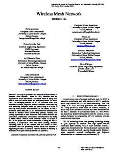
that a signal can be received on two link disjoint paths, such that if a link fails on one of the paths, the signal can still be received on the other path, where the backup path is shared. 3) Resuming data reception on the protection path is guaranteed to be within 1.5 times the propagation delay around a p-Cycle, but can be much less than this limit. In addition, and as a byproduct, in the absence of failures, this scheme provides an error recovery functionality in the absence of failures. This will be discussed in Section V. In this paper we introduce the basic concepts and theoretical bases of the strategy, and how it can be used to provide 1+N protection using p-Cycles against single link failures. We discuss the implementation of this scheme in a number of technologies and layers in Section VI. The rest of the paper is organized as follows. In Section II we provide a brief background on p-Cycles and network coding. In Section III we introduce a few operational assumptions. We illustrate the basic concept of our strategy by giving an example of using network coding to provide protection against a single link failure in Section IV. In Section V we show the general strategy for encoding and decoding data units on pCycles in order to provide protection for bidirectional unicast connections using one bidirectional p-Cycle. We illustrate this procedure using an example. We also outline the advantages of this scheme, as well as other uses for this scheme, especially in error control. In Section VI we discuss the issue of timing and synchronization of encoded and decoded data, and we show that the outage time, which is the time between the loss of the direct signal, and the recovery of the same signal on the protection path, is limited to no more than 1.5 times the delay on the p-Cycle. Some other implementation considerations, as well as notes on implementing this strategy in different technologies and protocols will also be discussed. A hybrid 1+N and 1:N protection scheme is introduced in Section VII in order to enable the p-Cycle to protect transmissions carried on the links used by the cycle itself. Section VIII shows some extensions to the proposed strategy which enables it to work with multipoint sessions. In Section IX we introduce an empirical comparison between 1+1 and 1+N protection. We also introduce a comparison between 1+1 and the hybrid scheme. The comparison is based on the cost of the network in terms of the number of links, and optimal formulations for these problems are given in the Appendices. Finally, in Section X we conclude the paper. II. BACKGROUND A. Background on p-Cycles The p-Cycle concept [2], [3], [4] is similar to the Bidirectional Line-Switched Ring (BLSR), since both of them have a cyclic structure. However, the p-Cycle concept has a higher protection coverage, since the spare capacity reserved on the cycle covers working capacity on the cycle, as well as working capacity on straddling links (see Figure 1). Since the protection capacity can be used to protect multiple connections, the p-Cycle belongs to the 1:N protection. The endpoints of

C

C

C B

D

G

B

D

A

E

A

F (a)

G

E

E

A

D

B

F (b)

F (c)

Fig. 1. p-Cycle concept: (a) a cycle (thick lines) traversing nodes A-G, and protecting circuits (thin lines) on the same physical path as the cycle, and on straddling paths; (b) prtection of a failure on the cycle; (c) protection of a failure on a straddling path.

the failure are responsible for detecting the failure, and for rerouting the traffic on the p-Cycle. There are two types of p-Cycles: link p-Cycles, which are used to protect the working capacity of a link, and this is the type shown in Figure 1, and node-encircling p-Cycles, which protect paths traversing a certain node against the failure of such a node. p-Cycles are embedded in mesh networks, and several algorithms have been introduced in the literature to select the p-Cycles which consume the minimum amount of spare capacity, e.g., see Chapter 10 in [4]. p-Cycles are very efficient in protecting against link failures, and the protection capacity reserved by p-Cycles achieves an efficiency that is close to that achievable in mesh-restorable networks. However, the preprovisioning of spare capacity makes p-Cycles much faster to recover from network element failures. p-Cycles can be used at a number of layers including the Optical layer, the SONET layer, or the IP layer [5]. Recently, p-Cycles have been extended from protecting spans or segments of flows, to protect entire flows, i. e., endto-end connections, regardless of the actual location of failure on the connection’s working path, hence the name FailureIndependent Path-Protecting (FIPP) p-Cycles [6], [7]. This requires all connections to be mutually link disjoint. In this case, if a connection is totally straddling or totally on the pCycle, a failure on the connection can be recovered from by switching the two end nodes of the connection to use the part of the p-Cycle that is disjoint from the connection (the entire p-Cycle in the case of a totally straddling connection, hence protecting twice as much working capacity on the straddling connections). However, if the connection is partly on the cycle and partly straddling, a failure is usually recovered from by using one default segment of the p-Cycle, unless the failure is on this segment; in the the latter case the complementary segment of the p-Cycle is used. This strategy leads to failureindependent end-to-end connection protection using a set of fully preconfigured protection circuits. In this paper we will use p-Cycles to protect a number of link disjoint connections, similar to FIPP p-Cycles, against failures. However, the protection will be done in 1+N manner, rather an 1:N. That is, our approach is to allow two transmissions of the same signal. One transmission is on the working path, and the second one is on a protection circuit, implemented by a p-Cycle. Multiple link disjoint connections

3 b

B b

b C

S a

a A

Fig. 2.

a+b

T2 a+b D a+b

a

T1

An example of network coding

transmit their signals simultaneously on the p-Cycle. The receivers receive these two copies, and select the better of the two signals. The backup signals are transmitted simultaneously and on the same protection circuit using the technique of network coding. Our approach can also be used at a number of layers including the SONET layer, especially Next Generation SONET, ATM, MPLS/GMPLS and IP. B. Background on Network Coding Network coding refers to performing linear coding operations on traffic carried by the network at intermediate network nodes. In this case, a node receives information from all, or some of its input links, encodes this information, and sends the information to all, or some of its output links. This approach can result in enhancing the network capacity, hence facilitating the service of sessions which cannot be otherwise accommodated. This is especially true when service mode is multicast. An example of the use of network coding is shown in Figure 2 in which node S transmits to nodes T1 and T2, and each link in the network has a capacity of one data unit per time unit. Data units a and b are delivered to both T1 and T2 by adding a and b at node C, where the addition is modulo 2. Both a and b are recovered at T1 and T2 by adding the explicitly received data units (a and b, respectively), to a+b. The network can then achieve a capacity of two data units per time unit. The concept of network coding for multicast sessions was introduced in the seminal paper by Ahlswede et al. [8]. The problem of network coding was formulated as a network flow problem in [9] and a link cost function was included in the formulation in [10]. Reference [11] introduced an algebraic characterization of linear coding schemes that results in a network capacity that is the same as the max-flow min-cut bound, when multicast service is used. The authors show that failures can be tolerated through a static network coding scheme under multicasting, provided that the failures do not reduce the network capacity below a target rate. Reference [12] introduced deterministic and randomized algorithms for the construction of network codes, which had polynomial time complexity. The algorithms could be used for multiple multicast sessions, where intermediate nodes may decode, and re-encode the received information. Reference [13] includes an introduction to network coding principles. Our objective in this paper is to use network coding with a group of unicast sessions in order to provide protection for such connections. III. O PERATIONAL A SSUMPTIONS In this section we introduce a number of operational assumptions.

• In this work we deal with connections. A connection may consist of a circuit on a single link, or may consist of a sequential set of circuits on multiple links, e.g., a lightpath. Therefore, link protection is a special case of this technique. • The term link is used to refer to a fiber connecting two nodes. Each link contains a number of circuits, e.g., wavelength channels, or even channels with smaller granularities, e.g., DS3. • A p-Cycle protecting a number of connections passes through all end nodes of such connections, similar to FIPP p-Cycles. In doing so, the p-Cycle protects connections with the same transport capacity unit, e.g., DS-3. Therefore, the p-Cycle links themselves have the same transport capacity. • The p-Cycle is terminated, processed, and retransmitted at all end nodes of the connections. • We assume that all connections are bidirectional, and connections that are protected by the same p-Cycle are mutually link disjoint. • It is assumed that data units are fixed in size1 . • The scheme presented in this paper is designed to protect against a single link failure. That is, when a link fails, it will be protected, and will be repaired before another link fails. • When a link carrying active circuits fails, the tail node of the link is capable of identifying the failure in some way, e.g., by receiving empty data units. This paper presents the concepts of using network coding on p-Cycles to achieve 1+N protection. It is to be noted that this strategy can be implemented using a number of layers and protocols, including the GFP [14] protocols of NGS, where data units to be treated like packets by GFP. The strategy can also be implemented using ATM, MPLS or IP. It should be pointed out that all addition operations (+) in this paper are over GF(2), i.e., as modulo two additions, i.e., Exclusive-OR (XOR) operations. IV. A N I LLUSTRATIVE E XAMPLE In this section we illustrate our basic idea using a simple example. As stated above, our objective is to provide each destination with two signals on two link disjoint paths, such that the network can withstand any single link failure. For the sake of exposition, we first consider unidirectional connections, and then extend it to bidirectional connections. The example is shown in Figure 3.(a), and there are three unidirectional connections from source Di to destination Ui , for i = 1, 2, 3. To simplify the example, we assume that all sources and their corresponding destinations are ordered from left to right. Assume that each connection requires one unit of capacity. Let us also assume that data units d1 , d2 and d3 are sent on those connections. A p-Cycle is preconfigured to include all the three sources and destinations, as shown in the figure. Data units di will be transmitted three times: once on the primary working path, and twice, and in opposite directions on the p-Cycle. One of the transmissions on the p-Cycle is by the original transmitter of the data unit, Di , and the other by the receiver, Ui . To distinguish between those last two data 1 The

case of variable size data units will be discussed in Section VI.

4 r u3 t u3

r r u3+u2 t t d1+d2

t d1 D1

D2

d1

d2

U1

U2

t d1

t t d1+d2

r d1

t t t d1+d2+d3

t t t u3+u2+u1

t t u3+u2

D3

D1

D2

d3

u1

u2

u3

U1

U2

U3

U3 t t t u3+u2+u1

t t u3+u2

D3

t u3

r r d1+d2 (a)

(b)

Fig. 3. An example of the use of network coding on p-Cycles to protect against single link failures: (a) the sources are at Di , and the destinations are at Di nodes; (b) the source are at Di , and the destinations are at Di nodes.

units we refer to them as transmitted and received di units, viz., dti and dri , respectively. On the p-Cycle, the following takes place: 1) Node D1 transmits dt1 in the clockwise direction. Node D2 will add its own data unit, dt2 to dt1 which it receives on the p-Cycle, where the addition is modulo 2, and transmits dt1 + dt2 on the p-Cycle, also in the clockwise direction. Node D3 will repeat the same operation, and will add dt3 to dt1 + dt2 , and transmits the sum on the p-Cycle. That is, node U3 receives dt1 + dt2 + dt3 on the p-Cycle, and in the clockwise direction. 2) On the same direction of the p-Cycle, but at the destinations, when destination U3 receives dt1 + dt2 + dt3 , and receives d3 on the working path, it adds d3 to dt1 +dt2 +dt3 to obtain dt1 + dt2 , and forwards it to U2 . Node U2 will also add d2 , which it receives on the working path, to dt1 + dt2 to recover dt1 , which it transmits on the same p-Cycle to U1 . U1 removes dt1 from the clockwise cycle. 3) Also, when node U1 receives d1 on the working path, it sends it on the p-Cycle, but in the counter-clockwise direction. It will be referred to as dr1 . Node U2 , when it receives d2 on the working path, it adds it to dr1 , and transmits dr1 + dr2 on the p-Cycle, also in the counterclockwise, direction. Based on the above, it is obvious that in the absence of failures, each destination node, Ui , for i = 1, 2, 3, receives two copies of di : 1) One copy on the primary working path, P and i 2) The second copy is obtained by adding j=1 dtj which Pi−1 r it receives on the clockwise p-Cycle to j=1 dj , which is receives on the counter-clockwise cycle. This is what we refer to a virtual copy of di . In this case, timing considerations have to be taken into account, as will be discussed in Section VI. When a failure occurs, it will affect at most one working path, e.g., working path i. In this case, we assume that Ui will receive an empty data unit on the working path. Therefore, Ui will be able to recover di by using virtual copy Pithe second P i−1 r t described above, i.e., by adding d and j=1 dj . A j=1 j failure on the p-Cycle will not disrupt communication. The case in which information is sent in the opposite direction, i.e., from Di to Di is shown in Figure 3.(b). Data

units in this case are labeled ui , and similar to di data units, uti and uri distinguish between newly transmitted and received ui data units. We refer to a bidirectional p-Cycle as a full cycle, and a one directional cycle is a half p-Cycle. In each of the above two examples, less than a full p-Cycle is used. In order to support bidirectional communication, the two approaches above have to be combined. In this case, less than three half p-Cycles, or 1.5 full p-Cycles are used. That is, one half p-Cycle (the outer one) is shared by both dri and uri data units. However, this can be accomplished because of the ordering of Di and Ui that we enforced in this example. In the general case where Di and Ui can be arbitrarily ordered, as will be shown next, combining the two bidirectional sessions would require two full p-Cycles. However, by linearly combining ui and dj signals on the same link and in the same direction, it is possible to reduce the number of p-Cycles to one full cycle, hence the name 1+N protection, where one full p-cycle is used for protection N connections. This will be illustrated in the next section. V. N ETWORK C ODING S TRATEGY

ON P -C YCLES

In this section we introduce our general strategy for achieving 1+N protection in mesh networks using p-Cycles. A. The Strategy In the examples shown in the previous section, we presented a special case in which the working connections were ordered from left to right. However, in this section we introduce a strategy for general connections. We assume that there are N bidirectional unicast connections, where connection i is between nodes Ai and Bi . We define the sets A = {Ai |1 ≤ i ≤ N } and B = {Bi |1 ≤ i ≤ N }2 . We denote the data units transmitted from nodes in A to nodes in B as d units, and the data units transmitted from nodes in B to nodes in A as u units. Before describing the procedure, it should be pointed out that the basic principle for receiving a second copy of data unit, e.g., u′i by node Ai , is to receive on two opposite directions the signals given by the following two equations: X u′j (1) j, Aj ∈A′

u′i +

X

u′j

(2)

j, Aj ∈A′

for some A′ ⊂ A, Ai ∈ / A′ , where data unit u′j is the one to be received by Aj , and the sum is modulo 2. In this case, Ai can recover u′i by adding equations (1) and (2) using modulo 2 addition also. Our procedure goes through the following steps: A.1 p-Cycle Construction and Node Assignment to Cycles: 1) Find a full p-Cycle. The full p-Cycle consists of two unidirectional half p-Cycles in opposite directions (more 2 Note that the choice of the labels A and B is arbitrary, as long as A i i i and Bi communicate with each other.

5

on this in item 3 below)3 . These two p-Cycles do not have to traverse the same links, but must traverse the nodes in the same order. 2) Construct two sequences of nodes, D = (D1 , D2 , . . . , DN ) and U = (U1 , U2 , . . . , UN ) of equal lengths, N . All elements of D and U are in C = A ∪ B, such that if two nodes communicate, then they must be in different sequences. We use the simple procedure shown in Algorithm 1 to construct the sequences. Algorithm 1: Algorithm for constructing the sequences D and U Initialization: D = U = ( ); //initialize empty sequences i = 1, j = N ; C = A ∪ B; D1 = A1 ; // select first node in D, and traverse p-Cycles i = i + 1; C = C − {A1 }; while C 6= φ do c = next node on p-Cycles in clockwise direction; if c communicates with a node in D then Uj = c; j = j − 1; else Di = c; i = i + 1; C = C − {c}; We arbitrarily select the sequence of nodes in D to be in the clockwise direction, and the sequence of nodes in U to be in the counter-clockwise direction. We also start with any node4 in C as D1 , and we label this node as A1 . All nodes in D belong to the set A, and all nodes in U belong to the set B. Node U1 will always be the one to the left of node D1 . The example in Figure 4 shows how ten nodes, in five connections are assigned to D and U. A node Di in D (Ui in U) transmits di (ui ) data units to a node in U (D). 3) The two half p-Cycles are a clockwise half p-Cycle, and a counter-clockwise half p-Cycle, which are used as follows: a) A half p-Cycle in the clockwise direction, T. On this half cycle newly generated di units generated by nodes in D, and newly generated ui units generated by nodes in U are encoded and transmitted as dti and uti , respectively. The dti and uti data units are decoded and removed by the corresponding receivers in U and D, respectively. 3 We assume that such p-Cycles exist, but if they do not exist, we find the largest subset of connections for which such p-Cycles exist, and then apply the strategy to those connections. 4 The selection of the node to be labeled D is important in bounding the 1 delay to recover from lost data due to failures, and also the outage time. This issue will be discussed in Section VI.

b) A half p-Cycle in the counter-clockwise direction, R. On this half cycle, di units received on the primary working paths by nodes in U, and ui data units received, also on the primary working paths, by nodes in D are encoded and transmitted as dri and uri , respectively. The dri and uri data units are decoded and removed by the corresponding transmitters in D and U, respectively. Note that the encoding and decoding operations referred to above are simple modulo 2 addition operations of data units to be transmitted and the data units received on such cycles, as will be explained below. Transmissions occur in rounds, such that dti data units which are encoded together and transmitted on the p-Cycle must belong to the same round. uti data units encoded together mus also belong to the same round. Rounds on the T cycle can be started by the D1 node. Other nodes follow D1 and transmit their own di and ui data units which belong to the same round. Rounds in the R cycle are also started by node D1 , but node U1 is the first node to transmit in a round, followed by other nodes in the counter-clockwise direction. All nodes in D and U must keep track of round numbers. The same round number conditions apply to rounds in which sums of uti data units are transmitted, as well as rounds for transmitting sums of dri , and sums of uri data units. The handling of round numbers, and which data units to transmit in round n, will be explained in detail in Section VI-E. A.2 Encoding Operations: The network encoding operation is executed by the nodes in D and U as follows (assuming no link failures): 1) Node Di : a) The node will add the following data units to the signal received on T: t • Data unit di , which is newly generated by Di . t • Data unit uj , which is received on the primary path from Uj . The result is transmitted on the outgoing link in T. b) The node will add the following data units to the signal received on R, and will transmit the result on the outgoing link in R. r • Data unit di , which it transmitted in an earlier round. r • Data unit uj , which it received on the primary path from Uj . 2) Node Ui will perform similar operations: a) The node will add the following data units to the signal received on T: t • Data unit ui , which is newly generated by Ui , and t • Data unit dj , which is received on the primary path from Dj . The result is transmitted on the outgoing link in T. b) The node will add the following data units to the signal received on R: r • Data unit ui , which it transmitted in an earlier round.

6

r r ru4+u5 r r u2+u3+ + u1

t t 4+u5 u t t u3+ u2+

r r r r u1+u3+u4+u5 r+ d1

r r r r r u3+u4 u1+u3+u4 r r+ r r +r d1+d2+d3 d1+d2

t t t t t u3+u4 t t u1+u3+u4 + t t + t t t u1+u3+u4+u5 t t + d1+d2+d3 d1+d2 t d1

t u1+

D2

1 0

t u3 + t d1+dt2+ t t d3+d 4

t u3+ut5 + t d1+d t t 3+d4

ut5 d1t t + +d 3+ t d4 +d

D4

1 0 d3

1 0 d4

d2

1 0

r u5 + r d1+ r d3+ r r d4+ d5

u5

d1

1U5 0 0 1

t

D1

D3

r u3 r r + u3+u5 r r r r d1+d2+d3+d4 r +r r d1+d3+d4

5

d5

D5

11 00

1u1 0 0 1

T

U1

U2

R

1 U4 0

u3

1U3 0

t u1+ t u2+ t u

3+ut 4+ut 5

r u1+ r u2+ r u3+ r u4+ r u5

Fig. 4.

u4

u2

1 0

t d3 + t u2+ut3+ t t u4+u5

t t d1+d3 + t t t u3+u4+u5

r r r d3 d1+d3 r r+ r r r r+ r u2+u3+u4+u5 u3+u4+u5

t t t d1+d3+d5 + t t u4+u5 r r r d1+d3+d5 r+ r u4+u5

T t +td5 t dt 3+d4 d1+ + t u5

R r r r r d4+d5 d1+d3+ r+ u5

An example of the application of the network coding procedure to a p-Cycle.

Data unit drj , which it received on the primary path from Uj . Also, the result is transmitted on the outgoing link in R. To understand the encoding and decoding operations, we first define the following: • T (Di ): node in U transmitting and receiving from Di . • S(Ui ): node in D transmitting and receiving from Ui . ˆ x)n = sum of d data units transmitted by • D(T i D1 , D2 , . . . , Di in round n and by Di+1 , Di+2 , . . . , DN in round n − a on half cycle T which have not yet been removed by their corresponding receiver nodes in U. a is defined in equation (9), and is the cycle propagation delay in terms of packets. ˆ (T x)n = sum of u data units transmitted by • U i Ui , Ui+1 , . . . , UN in round n and by U1 , U2 , . . . , Ui−1 in round n − 1 on half cycle T which have not yet been removed by their corresponding receiver nodes in D. ˆ (Rx)n = sum of u data units received by • U i Di , Di+1 , . . . , DN in round n and by nodes D1 , D2 , . . . , Di−1 in round n − 1 and transmitted on half cycle R which have not yet been removed by their corresponding receiver nodes in U. n ˆ = sum of d data units received by • D(Rx) i U1 , U2 , . . . , Ui in round n and by nodes Ui+1 , Ui+2 , . . . , UN in round n − 1 and transmitted on half cycle R which have not yet been removed by their corresponding receiver nodes in D. Now, the above procedure can be explained as follows, with the help of the example in Figure 4: ˆ x)n ˆ x)n + U(T 1) In step 1a above, node Di receives D(T j i−1 on the incoming link on T. Node Uj is the node next to Di in the counter-clockwise direction. For example, for D2 in Figure 4, it is U1 , and for D5 , it is U5 . ˆ x)n , and The addition operations will add di to D(T i−1 n ˆ will remove uT (Di ) from U (T x)j . This will result in ˆ x)n + U ˆ (T x)n at the output of node Di , which D(T i j •

will be transmitted on the outgoing link on T. Node D3 in Figure 4 adds d3 , which is transmitted on the outgoing link. However, adding u1 , where T (D3 ) = U1 , removes it and is therefore not transmitted on T. n ˆ ˆ (Rx)n + D(Rx) 2) Also, in step 1b, node Di receives U j i+1 on the incoming link on R. Node Uj is the node in U which is next to Di in the clockwise direction. For example, in Figure 4, for D3 it is U5 , and for D5 , it is U4 . After the addition operation, uT (Di ) is added, and n ˆ (Rx)n + D(Rx) ˆ di is removed. The node outputs U i j on R. In Figure 4, at node D3 , the addition of d3 to the incoming signal on R removes it, while the addition of u1 , where U1 = T (D3 ) adds it to the signal which is transmitted on the outgoing link on R. ˆ x)n + D(T ˆ x)n on 3) In step 2a, node Ui receives U(T i+1 j the incoming link of T, where node Dj is the node in D next to Ui in the counter-clockwise direction. For example, in Figure 4, for U3 it is node D5 . The addition operation adds ui , and removes dj , where Dj = S(Ui ), ˆ x)n , which is transmitted ˆ (T x)n + D(T and produces U j i on the outgoing link of T. In Figure 4, U2 adds u2 , and removes d1 n ˆ 4) Finally, in step 2b, node Ui receives D(Rx) i−1 + ˆ (Rx)n on the incoming link of R, where Dj is the U j node next to Ui in the clockwise direction. For example, for U5 , it is D5 , and for U3 , it is D1 . The addition operation adds dj , and removes ui , where n n ˆ ˆ Dj = S(Ui ). The result is D(Rx) i + U (Rx)j , which is transmitted on the outgoing link of R. In Figure 4, U3 adds d5 , and removes u3 . A.3 Recovery from Failures: The strategy presented in this paper recovers from a single link failure on any of the N primary paths. Suppose that a link on the path between nodes Di and Uj fails. In this case, Di does not receive uj on the primary path. However, it can recover uj by adding

7

ˆ x)n + U ˆ (T x)n which is received on T, D(T i−1 j n n ˆ ˆ • U (Rx)i+1 + D(Rx) j , that it receives on R, and • di that it generated and transmitted earlier. For example, at node D3 in Figure 4, adding the signal received on T to the signal received on R, and d3 , then u1 can be recovered, since U1 = T (D3 ) generated u1 . Similarly, node Uj can recover di by adding ˆ (T x)n + D(T ˆ x)n which it receives on T, • U i+1 j n n ˆ ˆ • D(Rx) i−1 + U(Rx)j which is received on R, and • ui that it generated and transmitted earlier. Node U2 adds the signals on T and R, and the u2 it generated earlier to recover d1 . Note that the signals on T and R which are added together must have the same round number.

A. Timing Considerations

round n, ui units belonging to this round are added or deleted. The same thing applies to di units. Node D1 can start the first round on T, and the remaining nodes D and U follow. When data in the first round arrives at node U1 on the working circuits, it starts transmitting data received in round 1 on R, and all the nodes in U and D follow. Since primary paths are usually chosen as the shortest paths, therefore, data arriving at a destination node over the primary path will do so before data sent over the p-Cycle will arrive. Moreover, the primary path will have a delay which does not exceed τ , where τ is the propagation delay around the p-Cycle. Otherwise, the primary path will choose the shorter path over the cycle. There is a number of timing and delay issues that need to be considered: 1) Failure-Free Operation: Under the above assumption of the primary path being shorter than any secondary backup path, nodes in D and U will respectively receive their ui and di data units on the primary paths before they receive them on the backup paths. In this case, data units can be added to, and removed from the corresponding half p-Cycles without delay5 . 2) Operation Under Working Path Failure: Assume that the working path between nodes Di and Uk has failed. All other nodes will not be affected by this failure. Let us first consider the case of receiving di data units by Uk . Nodes in D can transmit their di data units on T in the corresponding cycles, and di data units must be removed by their corresponding receivers in U. This can be done by all nodes similar to case 1 above. However, for node Uk , di data units in cycle n received on T may have to be delayed at Uk until the corresponding combination of data units in cycle n on R arrive at Uk . To derive an upper bound on this delay, we now introduce a condition on the selection of nodes D1 and U1 : Find the two end nodes of a connection, such that on one sector of the p-Cycle, there is no connection that has its two end nodes on this sector. The end node of this connection, which is at the end of this sector in the counter-clockwise direction is taken as U1 , and the next node in the clockwise direction is taken as D1 . For example, in Figure 4, end nodes D3 and U1 of a connection have the sector that includes nodes D1 and D2 satisfy this condition. Therefore, the end node of this connection in the counter-clockwise direction is taken as U1 . Notice also that nodes D2 and U5 satisfy this condition, and node D2 could have been taken as U1 , while node D3 would have been labeled D1 in this case. Now we evaluate an upper bound on the delay time at node Uk , ∆Uk , which is the time that node Uk will have to delay data units on the T cycle. To illustrate the derivation, we will

For the above procedure to work properly, ui units added and removed at a node should be the same as those carried by the p-Cycle. For this reason, nodes operate in rounds, where in

5 In case the working path is longer than the backup path on the p-Cycle, the signals on the T half cycle can be delayed until the corresponding ui and di data units are received.

•

B. Advantages of the Proposed Strategy The proposed strategy has a number of advantages, which can be summarized as follows: • The strategy provides 1+N protection against single link failures, in which the protection resources are shared between connections, hence resulting in a potential reduction of the protection circuits over 1+1 protection. This is especially evident in cases where the nodal degree is high, e.g., four, such as in the NJ-LATA and Pan-European COST239 networks. • Similar to FIPP p-Cycles, the management plane will be simplified since it does not have to detect the location of the failure. • The control plane functionality will be simplified since it does not need to reroute the signals at any of the switches, including those at the end nodes of the failed connection, in order to recover from the failure. • Since signals will be received twice, and on two different paths, this strategy can also be used for error detection and correction in the absence of link failures. For example, if the two copies do not match, then this is an indication of an error. If the copy received on the working path is corrupted (which can be detected through the frame check sequence), then the copy recovered from the p-Cycle can be used instead. • Since data units are added together on the p-Cycle, data units encrypt each other, which provides a measure of security on the shared protection circuits at no additional cost. This requires that the number of connections protected by a p-Cycle be greater than 2. VI. I MPLEMENTATION C ONSIDERATIONS In this section we consider issues that need to be taken into account for implementing the above strategy. These include timing considerations, detection and removal of protection channel errors, security issues, and protocol implementation.

8 distance D1 time

U5

D5

U4

U3

U2

U1

τT D1,D3

d1

T τ D1,U5

D4

D3

D2

d1+d2 d1+d2+d3

ψ

d1+d2 +d3+d4

d1+d3

d3

d1+d3+d5 ∆

U5

d1+d3+d4

d1+d2+d3

d1+d2 +d3+d4

D3,U1

R

τ U1,U5

d1+d3 +d4+d5

d1+d3+d4 d1+d3 +d4+d5

d1+d2

d1+d3+d5 d1+d3

d1

d3

Fig. 5.

Example of the timing considerations, and delay at Uk nodes (Uk = U5 in this example).

use the space-time diagram in Figure 5, which corresponds to the example in Figure 4. In this figure, the p-Cycle is broken between nodes D1 and U1 , and the cycle is unrolled. It is also assumed that the connection between nodes D2 and U5 has failed, i.e., Di = D2 and Uk = U5 . The derivation is based on the following assumptions: • ψDj ,U1 is the delay over the working path from node Dj to node U1 . R • τU ,U is the delay between U1 and Uk on the R cycle. 1 k T • τD ,U is the delay between D1 and Uk on the T cycle, 1 k T and similarly is τD . 1 ,Dj • Since shortest path communication is used, the propagation delay between a pair of communicating nodes over the primary path is always shorter than that over either the T or the R cycles. • Node Dj is the one connected to node U1 . • Assume that a node transmits its data unit on the working circuit and the T cycle at the same time. Due to the last assumption, for a round to start on cycle R, a T delay of τD +ψDj ,U1 is required. This is shown in Figure 5, 1 ,Dj which is the space-time diagram corresponding to the example in Figure 4. In this example, node Dj is D3 . Hence, we have T T . + ψDj ,U1 + τUR1 ,Uk − τD Delay at Uk = ∆Uk = τD 1 ,Uk 1 ,Dj (3) The first two terms in the above equation correspond to the time from the start of a round on cycle T to the start of the same round on cycle R, as stated above. Then, we add to it the time for this round’s data to arrive at Uk on the R cycle (the third term). Finally, the time for the data in the same round to arrive at Uk on the T cycle is subtracted (the last term). By the choice of Dj , then

In the example in Figure 4, this delay is introduced at node U5 , assuming that the working circuit between nodes D2 and U5 in Figure 4 has failed. MSPP devices which can accommodate a 128ms differential delay, can support this implementation. Using the same method above, we obtain an upper bound on the outage time, which is the time between the loss of the direct signal, and the recovery of the same signal on the protection path. Using D1 as a references, the outage time at node Uk , ΘUk , is given by T T + ψDi ,Uk ) (6) + ψDj ,U1 + τUR1 ,Uk ) − (τD ΘUk = (τD 1 ,Di 1 ,Dj

The derivation of the above equation is similar to that of equation (3), except that we subtract the time from the beginning of the round to the reception of di by node Uk (the last term). Since any working path is shorter than τ /2, and since T + τUR1 ,Uk < τ τD 1 ,Dj

where we used the assumption of symmetry between the T and R cycles, then we have ΘUk < 1.5τ If the last assumption above is relaxed, and all nodes are synchronized to transmit on the working paths at the same time, e.g., using a network clock, then the first and fourth terms in equation (6) will disappear, and the delay will become Θ′Uk = (ψDj ,U1 + τUR1 ,Uk ) − ψDi ,Uk

(7)

This inequality is valid since if it was not, then Dj and U1 R will use τD as it will be shorter. j ,U1 Using equations (4) and (5) in equation (3) we obtain

which still has a loose upper bound of 1.5τ . In order to reduce the upper bound, and provide tighter guarantees on the outage time, all sources can start transmitting simultaneously, and at the same time both the T and R cycles can start. In order to make sure that the transmissions on the cycles will include valid data units, initially nodes are assumed to generate zero data units, which are not transmitted on the working paths, but are assumed to be received by the receivers. The number of such data units are those transmitted within a duration of maxi,j ψDi ,Uj . In this case, the outage time will be given by

∆Uk ≤ τ

T ) − ψDi ,Uk Θ′′Uk = max(τUR1 ,Uk , τD 1 ,Uk

T T − τD ≤0 τD 1 ,Uk 1 ,Dj

(4)

ψDj ,U1 + τUR1 ,Uk ≤ τ

(5)

Also,

(8)

9

which is upper bounded by τ . B. Synchronization Since data units that are to be combined together must belong to the same round, then all data units of the same round must be present in order to form the linear combination that will be transmitted on the outgoing link of a cycle. This requires the use of a synchronization mechanism. However, synchronization can be easily implemented based on the adoption of two mechanisms, namely: 1) Round numbers, and 2) Buffers that will hold data units that are to be combined, including the input linear combinations. The buffer, e.g., at node Di which has a connection to node Uj , will be used to hold transmitted di data units, received uj data units, and the linear combinations received on both T and R cycles. Once the data units belonging to the same round number are available at the head of their buffers, the output linear combination is formed and transmitted on the outgoing link. C. Nodal Degree and p-Cycles In order to implement the above scheme, each node should be able to transmit on three ports. If simple p-Cycles are used, then the implementation of this technique may not be feasible if source and/or destination nodes have a nodal degree of 2. However, since the on-cycle links are not protected, nonsimple cycles may be used. In fact, the use of non-simple cycles may even result in lowering the protection requirements, since a non-simple cycle that traverses a set of connection end nodes may require a number of links which is less than that required by simple cycles. D. Channel Errors The proposed scheme is robust with respect to channel errors, especially those which affect the composite signal. That is, once the composite signal is hit by an error burst, the error can be detected and removed, and this will take place within no more than two hops (of connection endnodes): one hop for detection, and a second hop for removal of the error. To see this, assume that an error burst hits the signal propagating on the T cycle just before it arrives at node Di , which has a connection with node Uj . Let this error burst be represented by the polynomial E. Therefore, ˆ x)n + U ˆ (T x)n + E on T, and node Di will receive D(T i−1 j n n ˆ ˆ U (Rx)i+1 + D(Rx)j on R. Let us consider two cases: Case 1: No Failures: In this case, the addition of the above two signals and the appropriate di and uj signals will result in E. Detecting that E is nonzero indicates an error. Since node Di does not know whether E has hit the signal received on T or the signal received on R, it only detects the error, but does not remove it. Therefore, it sends a short signal (can be a single bit) to both neighboring nodes to indicate the possibility of an error. The downstream node on T from Di will

detect the error again, and because of the receipt of this signal, it can now remove the error by adding E to the T signal. The upstream node on T from Di will not detect the error, and will therefore ignore the possible error indication signal received from Di . Case 2: A Working Path Failure: In this case, node Di will recover uj + E. Node Di can detect the presence of the error through the use of the CRC in the data unit. Notice that adding uj + E to the signal on T will remove both uj and E. However, in the general case, since node Di does not know which signal was hit by the error burst E, it will execute the same procedure in Case 1 by which it notifies its two neighboring nodes. E. Implementation Notes While this paper presents the theoretical bases of the proposed strategy, it is important to comment on the feasibility of implementing it. In fact, the proposed strategy can be implemented in a number of technologies and at a number of layers. For example, it can be implemented at layer 1 using NGS protocols, and in particular the GFP protocol. Since data units from different higher layer protocols are encapsulated in the payload field of GFP frames, the payload field can be used to accommodate the encoded (added) data units. It can also be implemented at layer 2 using ATM, where a special VCI/VPI can be reserved for a p-Cycle that protects a given set of VCCs or VPCs. The payloads of the ATM cells to be protected are therefore added and transmitted on the pCycle VCC. Moreover, it can be implemented at layer 3, and in particular using the IP protocol. With IP, the sum of data units (packets in this case) can be encapsulated in another IP packet. The encapsulating IP packet header would include the IP numbers (on two different interfaces) of the node that starts a round, e.g., D1 , as both the source and destination. Source routing may have to be used to make sure that this packet will traverse the p-Cycle. The strategy can also be implemented using MPLS where a certain LSP is used to implement the p-Cycle. All data units are added and the label of the p-Cycle LSP is prepended to the sum. In fact, with MPLS we have the advantage that paths are precomputed, and do not change during operation. Note that the proposed strategy requires four mechanisms: 1) Data units are fixed and equal in size, 2) Round numbers can be indicated in data units, 3) There is an XOR addition mechanism at each node, and 4) There is a buffer equal to the round trip delay around the p-Cycle at each node. The last two mechanisms are not difficult to provision. In order to implement the first mechanism, and if data units cannot be made fixed in size, e.g., under IP, a number of ways can be used to circumvent this problem. One option would be that each node would concatenate (or block) its own data units and then segment them into fixed size segments. Another option would be to use data units of a length that is equal to the data unit with the largest size. Shorter data units are extended by adding trailing zeroes. The first option

10

round number 01101

d1

d2

d3

d4

d5

u1

u2

u3

u4

u5

dj (n)) to T. Otherwise, it adds di (n)+uj (n−a) (ui (n)+ dj (n − a)). 1 1 0 0 0 0 0 0 0 0 • On R: node Di (Ui ) complements its round bit. If the round bit of node Uj (Dj ) is the same as that of the Fig. 6. The round number field, and an example showing how it is set when received by node D3 on the T cycle current node’s round bit, it adds di (n)+uj (n−a) (ui (n)+ dj (n − a)) to R. Otherwise, it adds di (n) + uj (n − 2a) (ui (n) + dj (n − 2a)). requires some processing, but is efficient in terms of bandwidth By doing this, node Di (Ui ) will guarantee that the two utilization. The second option, which is also feasible under a combinations arriving on the T and R cycles in round n number of technologies, can lead to bandwidth degradation correspond to the same combinations. since the bandwidth reserved for protection in this case will be based on the maximum size data units. However, since VII. H YBRID 1+N AND 1:N P ROTECTION it does not require blocking and segmentation, its processing requirements are less than those of the first option. Unlike p-Cycles used for 1:N protection, the 1+N protection Providing round number can be also accommodated in a scheme proposed in this paper does not protect circuits which number of technologies. For example, when using GFP, a new share links with the p-Cycle, i.e., on-cycle links. The reason extension header can be defined to include the round sequence is due to the use of network coding on the p-Cycle, which number. With IP, the sequence number of the encapsulating IP means that if an on-cycle link fails, the cycle will be broken, header can act as the sequence number. It is to be noted that and cannot be used to deliver the coded data to the end nodes data units combined on the T and R cycles can be offset by of the failed link. However, the 1+N protection scheme can a number of rounds that depends on a, where a is given by: be combined with the legacy p-Cycle 1:N protection scheme to protect circuits sharing links with the p-Cycle. In case a τ a=⌈ ⌉ . (9) working link on the p-Cycle fails, network coding will be (P rotection data unit size in bits)/B disabled, and the the circuits sharing links with the p-Cycle τ in the above equation is the round trip propagation delay can be rerouted on the p-Cycle, which requires end-node around the p-Cycle, and B is the protected transport capacity. switch reconfiguration. This will result in reducing the overall Considering the example of Figure 4, and if rounds on the protection redundancy. However, the failure recovery times for T cycle are started by node D1 , then at node D3 , if d1 and the 1:N protected circuits are expected to exceed those which d2 belong to round n, then u1 , u3 and u4 belong to round are protected by the 1+N scheme. We refer to this strategy as n − a. Therefore, the indication of the round number must a hybrid 1+N and 1:N protection. It should be noted that in also indicate the round number of each data unit. This can be the case when there are no straddling links, or circuits, this accommodated by including: hybrid strategy becomes the 1:N protection scheme. 1) The round number n, and In this section, we describe the basics of Hybrid 1+N/1:N 2) For each data unit, whether it belongs to round number protection scheme for link protection 7. All of the previous n, or to a preceding round number, as will be indicated operational assumptions still hold in this case. However, a pbelow. Cycle will be provisioned to protect on-cycle and straddling For this purpose, we propose a round number field that links. In addition to the nodes in D and T , which are at the includes the round number and one round number bit for each ends of straddling links, we define the set of nodes X . Node data unit. This last bit will be the same as the least significant Xi ∈ X is not at the end of a straddling link, but is an end node bit (LSB) in the round number if the data unit belongs to the of an on-cycle link only. We also define C(Di ) and C(Di ) as same round number, n, or the complement of the LSB if the the next node in the clockwise and counterclockwise directions data unit belongs to an earlier round number, n − a on T, or on the p-Cycle from node Di , respectively. Similarly, we n − 2a on R. Assuming that a is odd6 , then since a is added define C(Ui ), C(Ui ), C(Xi ) and C(Xi ). We denote the data to the round number field to update round numbers by D1 , units sent in round n on the on-cycle working links by node Di C C the round number bits for all nodes will contain the above to nodes C(Di ) and C(Di ) by si (n) and si (n), respectively. information. Figure 6 shows this field and how it is set for the Similarly, we define the data units sent by Ui and Xi in the C clockwise and counterclockwise directions as tC combined data units received by node D3 on the T. i (n), ti (n), C C The determination of which data unit to add to round n on xi (n) and xi (n), respectively. A node on the p-Cycle can be one of two types: the T and R cycles is as explained below. Let us assume that node Di (Ui ) communicates with node Uj (Dj ). Type 1: An end node of both an on-cycle link, and a straddling link. Nodes in D and U are of this type. • On T: node Di (Ui ) complements its round bit. If the Or, round bit of node Uj (Dj ) is the same as that of the Type 2: An end node of an on-cycle link only. Nodes in X current node’s round bit, it adds di (n) + uj (n) (ui (n) + are of this type. 6 a is assumed to be odd for simplicity. If a is even, since node D starts 1 As described earlier, one of the Type 1 nodes will start rounds rounds, it will have to complement all bits in the round number bits for all on the p-Cycle in both directions, T and R, which will be used nodes, by simply XORing a vector of 1’s with such bits. However, a does not need to correspond to the actual value of a, but can be taken as the smallest odd integer greater than or equal to the value given by equation (9).

7 The

scheme works with either straddling links or straddling paths.

11

in exactly the same way described in Section V. Without loss of generality, let D1 be the node to start the rounds: It will start round n on T by transmitting d1 (n), and will start round n on R without transmissions. Node U1 will be the first node to transmit on R in round n. A Type 1 node will do two things: 1) It will behave similar to an on-cycle node in the 1+N protection scheme described in Section V. The data units combined by the Type 1 nodes and transmitted on the p-Cycle are used to protect straddling links, are called Straddling Links Protection (SLP) data units. 2) If a Type 1 Di node does not receive a data unit on the T cycle, it assumes that the link on the T cycle between C(Di ) and Di has failed, and sends the sC i downstream on the T cycle (i.e., in a direction opposite to that of the working link) so that it can be received by node C(Di ). Also, if the node does not receive a data unit on the R cycle, it assumes that the link on R cycle between C(Di ) and Di has failed and sends sC i downstream on the R cycle, so that it can be received by C(Di ). In the above two cases, node Di also receives the data units from C(Di ) and C(Di ) on R and T, respectively. Node Ui will behave similarly. The data units which are used to protect on-cycle links are called On-Cycle Links Protection (OLP) data units. A Type 2 node, Xi ∈ X , will only perform Step 2 performed by Type 1 nodes only, and will transmit OLP data units only. Two more mechanisms are needed: 1) At any of the nodes on the cycle, SLP data units have transmission precedence on the cycle over OLP data units. 2) At the node that starts the cycles, D1 , SLP data units for round n are not generated unless SLP data units for round n − a are received, where a is given in equation (9). We show an example in Figure 7 of a p-Cycle protecting five nodes, four of Type 1, D1 , D2 , U1 , and U2 , and one node of Type 2, X1 . In the absence of failures, the data units transmitted on the working links are shown in Figure 7.(a), while the linear combinations carried on the T and R cycles are shown in Figure 7.(b). When a straddling link fails, e.g., between D1 and U2 shown in Figure 7.(b), the combinations received at D1 and U2 can be used to recover u2 and d1 , respectively. However, when an on-cycle link fails, e.g., between nodes X1 and D2 , the T cycle is used to carry sC 2 to X1 in the clockwise direction. Similarly, the R cycle is used to carry xC 1 data units to D2 , and in the counterclockwise direction. This is shown in Figure 7.(c). VIII. E XTENSIONS TO M ULTIPOINT C OMMUNICATION In this section we discuss how the proposed technique can be used to protect multipoint connections, viz., one-to-many and many-to-one. A. One-to-Many Sessions We illustrate the procedure for handling one-to-many, or multicast, sessions by considering the case of the transmission

r r d1+d2

r d1

t t d1+d2

t d1

r r r d1+d2+d3 t t t d1+d2+d3

D2

D3

D1

T

R

U5 U1 t d1 r d1

Fig. 8.

U4

U2

U3

t t d1+d2

t t t d1+d2+d3

r d1

r r d1+d3

t t t d1+d2+d3 r r d1+d3

t t t d1+d2+d3 r r r d1+d2+d3

1+N protection of multicast connections

of di units from node Di in D to multiple destination nodes in U. A similar procedure can be implemented for transmissions from a node on U to nodes in D. We denote by Uc and Uf the destinations in the session that are, respectively, the closest and the farthest from the session source in D on the T cycle in the clockwise direction. These two nodes have the following responsibilities: • Node Uc adds data units di to the R cycle. It does not act on the data received on the T cycle. • Node Uf removes data units di from the T cycle. It does not act on the data received on the R cycle. Based on the above, in the case of failure P all destination nodes in the multicast session will receive j,Dj ∈B,j6=i dj + di on P cycle T, and j,Dj ∈B,j6=i dj on cycle R, where B is a subset of D. This enables such destinations to recover the di units in case of failure. This is shown in the example in Figure 8 where D2 transmits data units d2 to U2 , U4 and U5 . The above may require buffering data on the T cycle at Uf until data in the corresponding round arrives from upstream on the R cycle. Or, it may require buffering data on the R cycle at Uc until data in the corresponding round arrives from upstream on the T cycle. Buffering at both nodes is not required. Note that the above strategy can tolerate the failure of multiple links on the multicast tree from Di to its destinations in U. B. Many-to-One Sessions In the case of many-to-one sessions, the adaptation of the proposed strategy is straightforward. In this case, the destination node can be regarded as multiple destinations, and it applies the basic strategies m times, where m is the number of sources in the session. Since the destination node will be receiving at a rate that is equal to the sum of the rates of all transmitters, the p-Cycle must operate at least at this rate. Therefore, data units transmitted by the sources of the same session can be time multiplexed on the p-Cycle. The paths from the sources to the destination need not be link disjoint. IX. C OST E VALUATION

OF

1+N P ROTECTION

In this section we evaluate the cost of 1+N protection using p-Cycles, and compare it to the cost of 1+1 protection. The cost evaluation of 1+1 and 1+N protection is based on optimal formulations. For the case of 1+1 protection, Bhandari’s algorithm [15] was used to find two links disjoint

12

C x 1 sC 1

D1

sC 2 C s 1

X1

d +u 1 1

u +u 1 2

C x 1

d +u 1 1

d +u 1 1

D2

1

X1

U1

C t 2 C t 1

(a)

U1

U2

D2

T

u 2

tC 1

D1

D2

C s 2

d 2

u 1

C s2

d +d 1 2

X1 D1

d

C x1

d +u 1 1

C t 2

R

T

U1

U3

u +u 1 2

R

U2

u +d 2 2

d +u 2 2

d +d 1 2

(b)

(c)

Fig. 7. An example of a p-Cycle used to protect 2 straddling and 5 on-cycle links: (a) the working links; (b) the protection circuits used to protect straddling links; (c) the protection circuits used to protect on-cycle links.

paths between the end nodes of each connection. An integer linear programming (ILP) formulation is used to evaluate the cost of 1+N protection. The ILP formulation is given in the appendix. These will be used to carry out an empirical comparison between the cost of implementing both strategies. It is to be noted that the cost metric used in this paper is the number of links, where a span may contain a number of links, e.g., DS-3 circuits or wavelengths. We compare the cost of implementing 1+1 and 1+N protection strategies using random graphs, while assuming that there is no upper bound on the number of links per span. In our experiments, we allow the use of non-simple cycles. Therefore, and due to the complexity of the problem, we ran our experiments using 8-node networks. The networks were generated randomly such that each sample network contained a given number of edges, and that the network is at least bi-connected. For the generated network, we provisioned a given number of connections, such that the end points of the connections were uniformly selected from all the nodes in the network. For each experiment, we generated 10 sample networks, and calculated the average of the number of protection and working circuits over all the runs. In the examples below, we show the total number of wavelength links, and between parentheses we show the number of protection and working circuits, respectively. In the first example, shown in the first half of Table I, the network has 8 nodes, and 12 edges. The average nodal degree in this case is 3. In the examples, we show the total network cost, and the cost of primary and protection paths. The table shows that 1+1 protection performs better than 1+N protection, both in terms of the number of working and protection circuits. Notice that when the number of connections is equal to the number of links in the graph (the case referred to as links), i.e., the case of link protection8, the number of working circuits is exactly the same in both cases, but the number of protection circuits is about 15% more in the case of 1+N. That is, 1+N protection has no advantages in this case. However, as the network becomes denser, 1+N protection requires fewer circuits than 1+1 protection. This is shown in the second half of Table I, where the nodal degree in this case is 4. Although the number of protection circuits exceeds the number of working circuits under 1+N protection, but the cost of protection circuits under 1+N protection is at least 30% lower 8 The connections were embedded in the ILP such that each of the |E| connections is routed over exactly one edge in the network graph.

than that under 1+1 protection. In Table II we show the cost of 1+1 and 1+N protection when link protection for all links in the network is provided. Four networks are considered, two six node networks, with 10 and 12 edges respectively, and two eight node networks, similar to those in Table I. In these examples, and similar to the conclusion drawn from the above two examples, it is shown that the cost of 1+N protection becomes less than the cost of 1+1 protection as the network density increases. It is to be noted that there is a large number of networks with a high nodal degree, i.e., 4 or more. Examples of which include the NJ-LATA with a nodal degree of 4, and the Pan-European COST239 network with a nodal degree of 4.7. Such networks may be regarded as candidates for the use of the proposed strategy. TABLE I C OMPARISON BETWEEN 1+1 AND 1+N PROTECTION IN AN 8- NODE NETWORK

|E|

12

16

N 12 (links) 10 8 16 (links) 14 12

Total 39 41 31 51 49 44

1+1 Working 12 16 12 16 19 18

Spare 27 25 19 35 36 26

Total 43 50 37 39 45 34

1+N Working 12 24 13 16 20 16

Spare 31 26 24 23 25 18

TABLE II F ULL LINK PROTECTION |V | 6 8

|E| 10 12 12 16

Total 30 36 39 51

1+1 Working 10 12 12 16

Spare 20 24 27 35

Total 30 26 43 39

1+N Working 10 12 12 16

Spare 20 14 31 23

One thing that was observed from the above results is that the maximum number of links per span under 1+N protection is less than under 1+1 protection. For example, for a network of 8 nodes and 12 edges, protecting 10 connections using 1+1 protection required several spans to be provisioned with 5 links on the same span. With 1+N protection, however, only one span needed to be provisioned with 4 links, and the rest were provisioned with either 1 or 2 links. This means that restricting the number of links per span to a certain upper bound may change the cost significantly. This is the subject of future study. It is to be also noted that the saving introduced

13

by 1+N protection over 1+1 protection is somewhat limited in this study. This is due to the use of small networks, which were the only networks that the ILP was able to solve in reasonable time. We also illustrate the cost of the Hybrid 1+N/1:N protection, and compare it to the cost of 1+1 protection. The cost of the Hybrid 1+N/1:N protection is based on using the ILP formulation which is similar to that in [16]. However, we modified the formulation in [16] in order to also maximize the number of links which are protected using 1+N protection, without resulting in increasing the number of protection circuits. Due to the lack of space, we do not include the ILP formulation in the paper. The experiments considered a number of networks where the number of nodes assumed two values, 8 and 14 nodes. We allowed the graph density for each network to assume one of four values, namely, 1, 1.5, 2 and 2.5. The graphs were generated randomly, but we made sure that all graphs were at least bi-connected. For each network, 8 different random graphs were generated, and we took the average of the results. In Table III, we show the cost of the protection circuits required for both 1+1 and Hybrid 1+N/1:N protection. For the Hybrid 1+N/1:N protection, the number of links which are protected as straddling links, i.e., using 1+N protection, is also shown. TABLE III C OMPARISON BETWEEN 1+1 AND HYBRID 1+N

|V | |E| 8 8 12 16 20 14 14 21 28 35

1+1 Protection protection cost 56 30 32 40 182 65 56 70

PROTECTION

Hybrid 1+N/1:N Protection protection cost # straddling links 8 0 9 4 8 8 8 12 14 0 16 6 20 19 15 24

Under 1+1 protection, the worst case cost of protection circuits is always when the nodal degree is 2, i.e., the network has a ring topology. There is exactly one way of choosing the protection path, namely, the entire ring topology excluding the protected link. However, under Hybrid 1+N protection, the problem reduces to p-Cycle protection, where all the protected links are on-cycle links, and the cycle corresponds to the entire graph. This results in the largest percentage of protection circuits, 100%. Note that in this case, for the Hybrid 1+N protection, there are no 1+N protected links, and it is 1:N protection. As the number of edges increases, and consequently the nodal degrees, the cost of 1+1 protection remains high, which is always around 200% of the cost of working links. Under Hybrid 1+N protection, the ratio of the protection circuits to the working circuits decreases. Notice also that as the number of edges increases, the number of links which are 1+N protected, i.e., straddling links, also increases. For example, with a graph density of 4, at least 50% of the links are protected using 1+N protection, since they are straddling links. The remaining links are 1:N protected.

X. C ONCLUSIONS This paper presented the principles of a scheme for achieving 1+N protection against single link failures by using network coding on p-Cycles. Data units are coded at sources and destinations, and transmitted in opposite directions on p-Cycles, such that when a link on the primary path fails, data can be recovered from the p-Cycle using simple modulo 2 addition. The strategy allows fast and graceful recovery from failures. It also simplifies the management and control planes, and can also provide a mechanism for error detection and correction. The scheme can be implemented at a number of layers and using a number of protocols including IP, or GFP in NGS. In order to protect on-cycle links, a hybrid 1+N/1:N strategy was presented in which on-cycle links are protected using 1:N protection. A performance evaluation study showed that as the density of the graph increases the efficiency of the proposed 1+N protection scheme improves in terms of decreasing the ratio of the required protection circuits compared to the working circuits. Moreover, the 1+N protection becomes more efficient than 1+1 protection under the same conditions. Therefore, the proposed strategy can be a candidate for use in networks with high average nodal degrees, such as NJ-LATA and the Pan-Eurpoean COST239 networks. Future work will consider implementing the proposed strategy in different technologies. It will also consider detailed performance evaluation and the effect of practical network dimensioning limitations on the performance. Moreover, since the ILP formulations presented in this paper have a high complexity, which limits their applicability to small networks, we plan to develop heuristic and approximate approaches, which may be sub-optimal, but may allow provisioning of larger numbers and a greater number of connections.

ILP FOR

THE

A PPENDIX M INIMAL C OST 1+N P ROTECTION

This appendix finds the minimal cost provisioning for 1+N protection in mesh networks using an ILP formulation. The cost is defined in terms of the number of wavelength links. It is assumed that the number of wavelength channels is not upper bounded. It is also assumed that wavelength conversion is available at all nodes, and therefore wavelength continuity is not enforced. In this case, several copies of the same p-Cycle may be needed. This is because two connections may have to be protected by the same cycle, but such connections cannot be routed on link disjoint paths. Multiple copies of the same p-Cycle must be routed on different wavelength channels, or different circuits, depending on the unit of protection. We start by finding the set of all cycles P in the network graph. The ILP formulation assumes that there are K copies of each cycle. The following table defines the parameters and variables used in the formulation: N number of connections (input parameters) s(k) source of connection k (input parameter) d(k) destination of connection k (input parameter) k Zij binary variable which is 1 if and only if connection k uses link (i, j) on primary path Pk subset of cycles that may be used to protect connection k, i.e., s(k) and d(k) are on a cycle in Pk

14

Lp p Ci,j

length of cycle p (input parameter) binary variable which is 1 if link (i, j) is on cycle p (input parameter) K number of copies of each cycle (input parameter) δkp,m binary variable which is 1 if copy m of cycle p is used by connection k ∆p,m binary variable which is 1 if copy m of cycle p is used Minimize: X X k Zi,j + ∆p,m Lp p,m

k,i,j k Zis

Subject to:

=0

∀k, i 6= s(k)

(10)

k Zdj =0 X

∀k, j 6= d(k)

(11)

k Zsi

=1

∀k

(12)

k =1 Zid

∀k

(13)

i6=s(k)

X

X

i6=d(k) k Zij =

i k Zij +

X

i k Zji

k Zji

∀k, j 6= s(k), d(k)

(14)

p p + δkp,m (Cij + Cji )≤1

∀i, j, k, p ∈ Pk , 1 ≤ m ≤ K (15) / Pk , 1 ≤ m ≤ K δkp,m = 0 ∀k, p ∈ X p,m δk = 1 ∀k δkp,m + P

k,

m,p∈Pk k k Zij + Zji

(16) (17)

l l + δlp,m + Zij + Zji ≤3

∀k, l, k 6= l, i, j, p, 1 ≤ m ≤ k (18) p,m X δ s.t. p∈Pk k ≤ ∆p,m ≤ δkp,m Q k, s.t. p∈Pk

∀p, 1 ≤ m ≤ K

(19)

Equations (10), (11), (12), (13), and (14) ensure that the traffic on the working path is generated and consumed by the source and destination nodes, respectively. Equation (15) makes sure that connection k and the cycle used to protect k are link disjoint. Equations (16) and (17) guarantee that there is only one cycle that will protect connection k, and this cycle is one of the cycles in Pk . Equation (18) ensures that if two connections share a link and are protected by the same cycle, they are protected by different copies of the same cycle. The number of copies of each cycle is evaluated in equation (19). R EFERENCES [1] D. Zhou and S. Subramaniam, “Survivability in optical networks,” IEEE Network, vol. 14, pp. 16–23, Nov./Dec. 2000. [2] D. Stamatelakis and W. D. Grover, “Theoretical underpinnings for the efficiency of restorable networks using preconfigured cycles (p-cycles),” IEEE Trans. on Communications, vol. 48, no. 8, pp. 1262–1265, 2000. [3] D. Stamatelakis and W. D. Grover, “Ip layer restoration and network planning based on virtual protection cycles,” IEEE Jour. on Selected Areas in Communications, vol. 18, no. 10, pp. 1938–1949, 2000. [4] W. D. Grover, Mesh-based survivable networks : options and strategies for optical, MPLS, SONET, and ATM Networking. Upper Saddle River, NJ: Prentice-Hall, 2004. [5] G. Shen and W. D. Grover, “Extending the p-cycle concept to path segment protection for span and node failure recovery,” IEEE Jour. on Selected Areas in Communications, vol. 21, pp. 1306–1319, Oct. 2003.

[6] A. Kodian and W. D. Grover, “Failure-independent path-protecting pcycles: Efficient and simple fully preconnected optical-path protection,” IEEE Jour. of Lightwave Technology, vol. 23, pp. 3241–3259, Oct. 2005. [7] W. D. Grover and A. Kodian, “Failure-independent path protection with p-cycles: Efficient, fast and simple protection for transparent optical networks,” in Proc. of 7th Intl Conf. on Transparent Optical Networks (ICTON 2005), July 2005. [8] R. Ahlswede, N. Cai, S.-Y. R. Li, and R. W. Yeung, “Network information flow,” IEEE Trans. on Information Theory, vol. 46, pp. 1204–1216, July 2000. [9] T. Ho, D. R. Karger, M. Medard, and R. Koetter, “Network coding from a network flow perspective,” in Intl. Symp. on Info. Theory, 2003. [10] D. S. Lun, M. Medard, T. Ho, and R. Koetter, “Network coding with a cost criterion,” in IEEE Int. Symposium of Information Theory, 2004. [11] R. Koetter and M. Medard, “An algebraic approach to network coding,” IEEE/ACM Trans. on Networking, vol. 11, pp. 782–795, Oct. 2005. [12] S. Jaggi, P. Sanders, P. A. Chou, M. Effros, S. Egner, K. Jain, and L. M. G. M. Tolhuizen, “Polynomial time algorithms for multicast network code construction,” IEEE Trans. on Information Theory, vol. 51, pp. 1973–1982, June 2005. [13] C. Fragouli, J.-Y. LeBoudec, and J. Widmer, “Network coding: An instant primer,” ACM Computer Communication Review, vol. 36, pp. 63– 68, Jan. 2006. [14] E. Hernandez-Valencia, M. Scholten, and Z. Zhu, “The generic framing procedure (gfp): An overview,” IEEE Communications, vol. 40, pp. 63– 71, May 2002. [15] R. Bhandari, Survivable Networks: Algorithms for Diverse Routing. Springer, 1999. [16] W. He, J. Fang, and A. Somani, “A p-cycle based survivable design for dynamic traffic in wdm networks,” IEEE Globecom 2005.