Nov 30, 2011 - can produce a wide range of fascinating quantum phases. [1,2,3]. .... model on the infinite 2D square lattice, described below, .... evidence for a first phase transition between the Néel an- ... excluded since the gs energy did in fact show some defi- .... Table 1: Number of fundamental CCM configurations.
EPJ manuscript No. (will be inserted by the editor)
Magnetic order in spin-1 and spin- 32 interpolating square-triangle Heisenberg antiferromagnets
arXiv:1111.7237v1 [cond-mat.str-el] 30 Nov 2011
P. H. Y. Li and R. F. Bishop School of Physics and Astronomy, The University of Manchester, Schuster Building, Manchester, M13 9PL, United Kingdom Received: date / Revised version: date Abstract. Using the coupled cluster method we investigate spin-s J1 -J2′ Heisenberg antiferromagnets (HAFs) on an infinite, anisotropic, two-dimensional triangular lattice for the two cases where the spin quantum number s = 1 and s = 23 . With respect to an underlying square-lattice geometry the model has antiferromagnetic (J1 > 0) bonds between nearest neighbours and competing (J2′ > 0) bonds between next-nearest neighbours across only one of the diagonals of each square plaquette, the same diagonal in each square. In a topologically equivalent triangular-lattice geometry, the model has two types of nearestneighbour bonds: namely the J2′ ≡ κJ1 bonds along parallel chains and the J1 bonds producing an interchain coupling. The model thus interpolates between an isotropic HAF on the square lattice at one limit (κ = 0) and a set of decoupled chains at the other limit (κ → ∞), with the isotropic HAF on the triangular lattice in between at κ = 1. For both the spin-1 model and the spin- 23 model we find a second-order type of quantum phase transition at κc = 0.615 ± 0.010 and κc = 0.575 ± 0.005 respectively, between a N´eel antiferromagnetic state and a helically ordered state. In both cases the ground-state energy E and its first derivative dE/dκ are continuous at κ = κc , while the order parameter for the transition (viz., the average ground-state on-site magnetization) does not go to zero there on either side of the transition. The phase transition at κ = κc between the N´eel antiferromagnetic phase and the helical phase for both the s = 1 and s = 23 cases is analogous to that also observed in our previous work for the s = 12 case at a value κc = 0.80 ± 0.01. However, for the higher spin values the transition appears to be of continuous (second-order) type, exactly as in the classical case, whereas for the s = 21 case it appears to be weakly first-order in nature (although a second-order transition could not be ruled out entirely). PACS. 75.10.Jm Quantized spin models – 75.30.Kz Magnetic phase boundaries – 75.50.Ee Antiferromagnetics
1 Introduction In recent years, the theoretical study of two-dimensional (2D) quantum spin systems has been intensely motivated by the fact that such models often describe well the properties of real magnetic materials of great experimental interest. It is an encouraging fact that experiments have often supported theoretical predictions or vice versa. Moreover, the study of frustration and quantum fluctuation in quantum spin-lattice systems has developed into an extremely active area of research. The interplay between frustration and quantum fluctuations in magnetic systems can produce a wide range of fascinating quantum phases [1,2,3]. Both effects are in principle capable of destabilising or completely destroying the magnetic order of the spin system. In turn this might then lead to the formation of a spin-liquid phase or be responsible for other quantum phenomena of similar significant interest. The driving force for the differentiated manifestation of the various kinds of possible quantum effects can, in principle, also come from Send offprint requests to:
the type and nature of the underlying crystallographic lattice, from the number and variety of the magnetic bonds, and from the magnitude of the spin quantum numbers of the atoms that reside on the atomic lattice sites [4]. It is thus of considerable interest to try to study the effects of each of these driving forces in turn for specific model Hamiltonians. A particularly well studied 2D model is the frustrated spin- 21 J1 -J2 model on the square lattice with nearestneighbour (NN) bonds (J1 ) and next-nearest-neighbour (NNN) bonds (J2 ), for which it is now well accepted that in the case where both sorts of bonds are antiferromagnetic (Ji > 0; i = 1, 2) there exist two antiferromagnetic phases exhibiting magnetic long-range order (LRO) at small and at large values of α ≡ J2 /J1 respectively. These are separated by an intermediate quantum paramagnetic phase without magnetic LRO in the parameter regime αc1 < α < αc2 , where αc1 ≈ 0.4 and αc2 ≈ 0.6. For α < αc1 the ground-state (gs) phase exhibits N´eel magnetic LRO, whereas for α > αc2 it exhibits collinear stripeordered LRO.
2
P. H. Y. Li, R. F. Bishop: Magnetic order in s >
As already noted above, the spin quantum number s can, both in principle and in practice, play an important role in the phase structure of strongly correlated spinlattice systems, which often display rich and interesting phase scenarios due to the interplay between the quantum fluctuations and the competing interactions. Varying the spin quantum number s can tune the strength of the quantum fluctuations and lead to fascinating phenomena [5]. A well-known example of such spin-dependent behaviour is the gapped Haldane phase [6] in s = 1 one-dimensional (1D) chains, which is not present in their s = 21 counterparts. Some recent studies on large-spin (i.e., s > 21 ) systems include: (a) the comparison of the Heisenberg antiferromagnet (HAF) on the Sierpi´ nski gasket with the corresponding HAFs on various regular 2D lattices, including the square, honeycomb, triangular and kagom´e lattices, for the cases s = 12 , 1, and 32 [7]; (b) the one-dimensional (1D) Heisenberg chain for both integral and half-odd integral values of s up to a value of 10 [8,9,10]; (c) the 2D J-J ′ model on the square lattice containing two different types of NN bonds, for values of s between 12 and 2 [5]; d) the 2D spin-anisotropic XXZ Heisenberg Hamiltonian for s = 1 [8,11,12,13]; e) the spatially anisotropic J1 -J1 ’J2 model on the 2D square lattice for values of s up to 4 [14,15]; (f) the spin-anisotropic J1XXZ -J2XXZ model for s = 1 [16]; (g) the pure J1 -J2 model for s = 1 [17]; (h) the 2D Union Jack model for s = 1 and s = 23 [18]; and the 2D Heisenberg model on the honeycomb lattice for s = 1 [19]. Another example that has been experimentally studied involves the investigation of the single-ion anisotropy energy in the 2D kagom´e lattice for the case s = 52 [20]. Also noteworthy in this context is the recent discovery of superconductivity with a transition temperature at Tc ≈ 26 K in the layered iron-based compound LaOFeAs, when doped by partial substitution of the oxygen atoms by fluorine atoms [21]. This finding has been followed by the rapid discovery of superconductivity at even higher values of Tc (& 50 K) in a broad class of similar quaternary compounds. Enormous interest has thereby been engendered in this class of materials. The very recent first-principles calculations [22] shows, for example, that the undoped parent precursor material LaOFeAs of the first material investigated in this oxypnictide class is well described by the spin-1 J1 -J2 model on the square lattice. We have previously used the coupled cluster method (CCM) [23,24,25] to study the magnetic order in a spinhalf interpolating square-triangle HAF (viz., the J1 -J2′ model) [26,27]. This is a variant of the well-known J1 -J2 model on the infinite 2D square lattice, described below, in which one half of the NNN J2 bonds are removed. In the present paper we further the investigation of the J1 -J2′ model by replacing the spin- 21 particles by particles with s = 1 and s = 23 . The 2D spin- 21 J1 -J2′ model has also been studied recently by other means [28,29,30,31], but we know of no other studies of the model for spins with spin quantum number s > 21 .
1 2
interpolating square-triangle magnetic models
(a)
(b)
(c)
Fig. 1: (colour online) J1 -J2′ model; – J1 ; - - - J2′ ; (a) N´eel state, (b) spiral state, (c) striped state.
2 The model The Hamiltonian of the J1 -J2′ model is written as X X si · sk si · sj + J2′ H = J1 hi,ji
(1)
[i,k]
where the operators si ≡ (sxi , syi , szi ) are the spin operators on lattice site i, with s2i = s(s + 1), and we consider here the cases s = 1 and s = 32 . On the square lattice the sum over hi, ji runs over all distinct NN bonds, but the sum over [i, k] runs only over one half of the distinct NNN bonds with equivalent bonds chosen in each square plaquette, as shown explicitly in Fig. 1. We shall be interested here only in the case of competing (or frustrating) antiferromagnetic bonds J1 > 0 and J2′ > 0, and henceforth for all of the results shown we set J1 ≡ 1. Clearly, the model may be described equivalently as a Heisenberg model on an anisotropic triangular lattice in which each triangular plaquette contains two NN J1 bonds and one NN J2′ bond. The model thus interpolates continuously between HAFs on a square lattice (J2′ = 0) and on a triangular lattice (J2′ = J1 ). Similarly, when J1 = 0 (or J2′ → ∞ in our normalization with J1 ≡ 1) the model reduces to uncoupled 1D chains (along the chosen diagonals on the square lattice). The case J2′ ≫ 1 thus corresponds to weakly coupled 1D chains, and hence the model also interpolates between 1D and 2D scenarios. As well as the obvious theoretical richness of the model, there is also experimental interest since it is also believed to well describe such quasi-2D crystalline materials as organic compounds containing BEDTTTF [32], for which with J2′ /J1 lies typically in the range from about 0.3 to about 1; and Cs2 CuCl4 [33], for which J2′ /J1 takes a value of about 6, thus making this material even quasi-1D. The J1 -J2′ model has only two gs phases in the classical case (corresponding to the limit where the spin quantum number s → ∞). For J2′ < 21 J1 the gs phase is N´eel ordered, as shown in Fig. 1(a), whereas for J2′ > 12 J1 it has spiral order, as shown in Fig. 1(b), wherein the spin direction at lattice site (i, j) points at an angle αij = J1 α0 + (i + j)αcl , with αcl = cos−1 (− 2J ′ ) ≡ π − φcl . The 2
J1 pitch angle φcl = cos−1 ( 2J ′ ) thus measures the deviation 2 from N´eel order, and it varies from zero for 2J2′ /J1 ≤ 1 to 1 ′ ′ 2 π as J2 /J1 → ∞, as shown later in Fig. 3. When J2 = J1 we regain the classical 3-sublattice ordering on the triangular lattice with αcl = 23 π. The classical phase transition at J2′ = 21 J1 is of continuous (second-order) type, with the gs energy and its derivative both continuous.
P. H. Y. Li, R. F. Bishop: Magnetic order in s >
In the limit of large J2′ /J1 the above classical limit represents a set of decoupled 1D HAF chains (along the diagonals of the square lattice) with a relative spin orientation between neighboring chains that approaches 90◦ . In fact, of course, there is complete degeneracy at the classical level in this limit between all states for which the relative ordering directions of spins on different HAF chains are arbitrary. Clearly the exact spin- 21 limit should also be a set of decoupled HAF chains as given by the exact Bethe ansatz solution [34]. However, one might expect that this degeneracy could be lifted by quantum fluctuations by the well-known phenomenon of order by disorder [35]. Just such a phase is known to exist in the J1 -J2 model [36,37] for values of J2 /J1 & 0.6, where it is the so-called collinear striped phase in which, on the square lattice, spins along (say) the rows in Fig. 1 order ferromagnetically while spins along the columns and diagonals order antiferromagnetically, as shown in Fig. 1(c). We investigate the possibility below whether a stripe-ordered phase may be stabilized by quantum fluctuations at larger values of κ for either of the cases s = 1 or s = 23 , in order to compare with the earlier s = 21 case for which we found [26] that such a gs phase might exist for high enough values of the frustration parameter κ, as discussed below. Thus, for the s = 12 case our own CCM calculations [26] provided strong evidence that the spiral phase becomes unstable at large values of the frustration parameter κ. In view of that observation we also used the CCM for the s = 1 2 case with the collinear stripe-ordered state as a model state. We found tentative evidence, based on the relative energies of the two states, for a second zero-temperature phase transition between the spiral and stripe-ordered states at a larger critical value of κc2 ≈ 1.8 ± 0.4, as well as firm evidence for a first phase transition between the N´eel antiferromagnetic phase and the helical phase at a critical coupling κc1 = 0.80 ± 0.01. The transition at κ = κc1 for the s = 12 case was found to be an interesting one. As in the classical (s → ∞) case, the energy and its first derivative appeared to be continuous (within the errors inherent in our approximations), thus providing a typical scenario of a second-order phase transition, although a weakly first-order one could not be excluded since the gs energy did in fact show some definite signs of a (weak) discontinuity in slope. Furthermore, the average on-site magnetization was seen to approach a value Mc1 = 0.025 ± 0.025 very close to zero on both sides of the transition, but with a very sharp drop and hence a possible discontinuity in M on the spiral side of the transition, as is often more typical of a first-order transition. A particular interest here is to compare and contrast the corresponding transition(s) between the s = 12 and the s > 21 models. By contrast with the s = 21 we shall find below that for the cases with s = 1 and s = 32 the average on-site magnetization at the analogous phase transition between N´eel-ordered and spirally-ordered states approaches smoothly the same nonzero value on both sides of the transition. Such continuous phase transitions where the order parameter does not vanish are well known in quantum magnetism. A prototypical example is the s = 21
1 2
interpolating square-triangle magnetic models
3
anisotropic XXZ model with a Hamiltonian given by X (sxi sxj + syi syj + ∆szi szj ), (2) H =J hi,ji
and which thus contains only NN anisotropic, antiferromagnetic (J > 0) Heisenberg bonds. Classically (corresponding to the s → ∞ limit) the model has a continuous phase transition at ∆ = ∆c ≡ 1 between two different N´eel antiferromagnetic phases, one aligned along the z-axis for ∆ > 1, and the other along some arbitrary direction in the perpendicular xy-plane for −1 < ∆ < 1. The s = 21 model may also be solved exactly on a 1D chain by the Bethe ansatz technique [38]. It is found in this 1D case that as the critical point is approached, ∆ → ∆c = 1, from either side, the average on-site (or staggered) magnetization M → Mc = 0. The approach to zero is of a quite nontrivial kind, via a function with an essential singularity at ∆ = ∆c . By contrast, for the same s = 12 XXZ model of Eq. (2) on a 2D square lattice, M → Mc ≈ 0.31 as ∆ → ∆c = 1. Thus, the type of phase transition we observe below for the spin-1 and s = 23 2D interpolating square-triangle Heisenberg antiferromagnets is quite analogous to the one at ∆ = ∆c = 1 in the s = 21 XXZ model on the 2D square lattice, but not to that of the same XXZ model on the 1D chain. We now first briefly describe the main elements of the CCM below in Sec. 3, where we also discuss the approximation schemes used in practice for the s = 12 case and the s > 21 cases. Then in Sec. 4 we present our CCM results based on using the N´eel, spiral and striped states discussed above as model states (or starting states). We conclude in Sec. 5 with a discussion of the results.
3 The coupled cluster method The CCM (see, e.g., Refs. [23,24,25] and references cited therein) is regarded as one of the most powerful and most versatile modern techniques in quantum many-body theory. It has been successfully applied to many quantum magnets (see Refs. [4,25,36,37,39,40,41,42,43,44]) and references cited therein). The CCM is suitable for studying frustrated systems, for which the main alternative methods are often only of limited usefulness. For example, quantum Monte Carlo techniques are usually restricted by the sign problem for such systems, and the exact diagonalization method is limited in practice, especially for s > 21 , to such small lattices that it is often insensitive to the details of any subtle phase order present. The CCM method to solve the gs Schr¨odinger ket and bra equations, H|Ψ i = E|Ψ i and hΨ˜ |H = EhΨ˜ | respectively is now briefly outlined (and see Refs. [9,23,24,25,39, 40] for further details). The implementation of the CCM is initiated by the selection of a model state |Φi on top of which to incorporate later in a systematic fashion the multispin correlations contained in the exact ground states |Ψ i and hΨ˜ |. The CCM employs the exponential ansatz, ˜ −S . The creation correla|Ψ i = eS |Φi and hΨ˜ | = hΦ|Se P + tion operator S is written as S = I6=0 SI CI with its
4
P. H. Y. Li, R. F. Bishop: Magnetic order in s >
P destruction counterpart as S˜ = 1 + I6=0 S˜I CI− . The operators CI+ ≡ (CI− )† , with C0+ ≡ 1, have the property that hΦ|CI+ = 0 = C0− |Φi ; ∀I 6= 0. They form a complete set of multispin creation operators with respect to the model state |Φi. The calculation of the ket- and brastate correlation coefficients (SI , S˜I ) is performed by re¯ ≡ hΨ˜ |H|Ψ i to quiring the gs energy expectation value H be a minimum with respect to each of them. This results in a coupled set of equations hΦ|CI− e−S HeS |Φi = 0 and ˜ −S HeS − E)C + |Φi = 0 ; ∀I 6= 0, which we norhΦ|S(e I mally solve by using parallel computing routines [45] for the correlation coefficients (SI , S˜I ) within specific truncation schemes as outlined below. In order to treat each lattice site on an equal footing a mathematical rotation of the local spin axes on each lattice site is performed such that every spin of the model state aligns along its negative z-axis. As a result, our description of the spins is given wholly in terms of these locally defined spin coordinate frames. The multispin creation op+ + erators may be expressed as CI+ ≡ s+ i1 si2 · · · sin , in terms + of the locally defined spin-raising operators si ≡ sxi + syi on lattice sites i. Upon solving for the multispin cluster correlation coefficients (SI , S˜I ) as outlined above, the gs energy E may then be calculated from the relation E = hΦ|e−S HeS |Φi, and the gs staggered magnetization PN M from the relation M ≡ − N1 hΨ˜ | i=1 szi |Ψ i in terms of the rotated spin coordinates. If a complete set of multispin configurations {I} with respect to the model state |Φi is included in the calculation ˜ then the CCM forof the correlation operators S and S, malism becomes exact. However, it is necessary in practical applications to use systematic approximation schemes to truncate them to some finite subset. For the s = 21 case, the localised LSUBn scheme is commonly employed, as in our earlier paper on the s = 21 version of the present model [26], as well as in our other previous work [9,25,39,40,43]. Under this truncation scheme all possible multi-spin-flip correlations over different locales on the lattice defined by n or fewer contiguous lattice sites are retained. A cluster is defined as having n contiguous sites if every one of the n sites is adjacent (as a nearest neighbour) to at least one other. Clearly this definition, however, depends on how we choose the geometry of the lattice among various topologically equivalent possibilities that may exist. For example, the current model may be construed as referring to sites on a square lattice, as shown in Fig. 1. In this case the J2′ bonds, for example, join NNN sites (which, by definition, are thus not adjacent). Alternatively, the model may be equivalently construed as referring to sites on a triangular lattice, in which case both J1 and J2′ bonds join NN (and hence adjacent) sites. In all of the results presented here we consider the model to be defined on a triangular lattice in making CCM approximations. However, we note that the number of fundamental LSUBn configurations for s > 12 becomes appreciably higher than for s = 21 , since each spin on each site i can now be raised up to 2s times by the spin-raising oper1 ator s+ i . Thus, for the s > 2 models it is more practi-
1 2
interpolating square-triangle magnetic models
Table 1: Number of fundamental CCM configurations (Nf ) for the SUBn-n (n = {2, 3, 4, 5, 6, 7}) scheme for the N´eel and striped model states, for the J1 -J2′ model defined on a triangular lattice, for the spin-1 and spin- 32 cases.
Method
s=1
s=
Nf
3 2
Nf
SUBn-n
striped
spiral
striped
spiral
SUB2-2 SUB3-3 SUB4-4 SUB5-5 SUB6-6 SUB7-7
2 4 60 175 2996 11778
4 26 189 1578 14084 131473
2 4 60 175 3622 13320
4 27 211 1908 18501 188326
cal, but equally systematic, to use the alternative SUBnm scheme, in which all correlations involving up to n spin flips spanning a range of no more than m contiguous lattice sites are retained [15,16,18,25,41]. We then set m = n, and hence employ the so-called SUBn-n scheme. More generally, the LSUBm scheme is thus equivalent to the SUBn-m scheme for n = 2sm for particles of spin s. For s = 21 , LSUBn ≡ SUBn-n; whereas for s > 12 , LSUBn ≡ SUB2sn-n. The numbers of such fundamental configurations (viz., those that are distinct under the symmetries of the Hamiltonian and of the model state |Φi) that are retained for the N´eel and striped model states of the current s = 1 and = 23 models at various SUBn-n levels, defined with respect to an underlying triangularlattice geometry, are shown in Table 1. Although we never need to perform any finite-size scaling, since all CCM approximations are automatically performed from the outset in the N → ∞ limit, where N is the total number of lattice sites, we do need as a last step to extrapolate to the n → ∞ limit in the truncation index n. We use here the well-tested [15,16,26,40,41] empirical scaling laws E/N = a0 + a1 n−2 + a2 n−4 ,
(3)
M = b0 + b1 n−1 + b2 n−2 ,
(4)
exactly as we did previously for the corresponding s = 21 model [26], for the gs energy per spin E/N and the gs staggered magnetization M , respectively.
4 Results The results of the CCM calculations are reported here for the spin-1 and spin- 23 J1 -J2′ model Hamiltonian of Eq. (1), using the N´eel, spiral and striped states shown in Fig, 1(a)-(c) as CCM model states, and with the SUBn-n approximation scheme defined with respect to an underlying triangular-lattice geometry. We set the parameter J1 = 1. Our available computational power at present is such that we can perform SUBn-n calculations for the spiral model
P. H. Y. Li, R. F. Bishop: Magnetic order in s >
state (viz., the state that requires the highest number of fundamental configurations (Nf ) for a given SUBn-n truncation index n) only for values n ≤ 7 for both the s = 1 and s = 23 cases. We thus present results for each of the N´eel, striped and spiral states only up to the SUB7-7 level, for the sake of consistency in our extrapolations to the n → ∞ limit . We note that, as has been well documented in the past [46], the LSUBn (or SUBn-n) data for both the gs energy per spin E/N and the average on-site magnetization M converge differently for even-n sequences and odd-n sequences, similar to what is frequently observed in perturbation theory [47]. Since, as a general rule, it is desirable to have at least (n + 1) data points to fit to any fitting formula that contains n unknown parameters, we prefer to have at least 4 results to fit to Eqs. (3) and (4). Both the available odd and even series of our SUBn-n data violate this desirable rule. However, our results (for both sets n = {2, 4, 6} and n = {3, 5, 7}) for the s = 21 case are consistent with those using the larger LSUBm sequences available in this case. This gives us confidence in both the accuracy of our results and the robustness of our extrapolation schemes. Hence, for most of our extrapolated results below we use the even SUBn-n sequence with n = {2, 4, 6} and the odd SUBn-n sequence with n = {3, 5, 7}. Firstly, the results obtained using the spiral model state are reported. For this state we first perform CCM calculations with the pitch angle φ as a free parameter. At each separate level of approximation we then choose the angle φ = φSUBn−n that minimizes the energy ESUBn−n (φ). Classically we have a second-order phase transition from N´eel order (for κ < κcl ) to helical order (for κ > κcl ), where κ ≡ J2′ /J1 , at a value κcl = 0.5. By contrast, our CCM results presented below show that there is a shift of this critical point to a value κc ≈ 0.615 ± 0.010 in the spin-1 quantum case and κc ≈ 0.575 ± 0.005 for the spin- 23 quantum case, first indications of which are seen in Figs. 2 and 3. In both cases this is a second-order phase transition from N´eel-ordered to helically-ordered states. Thus, for example, curves such as those shown in Fig. 2 show that the N´eel state (φ = 0) gives the minimum gs energy for all values of κ < κc , where κc depends on the level of SUBn-n approximation used, as we also observe in Fig. 3. By contrast, for values of κ > κc the minimum in the energy is found to occur at a value φ 6= 0. If we consider the pitch angle φ itself as an order parameter (i.e., φ = 0 for N´eel order and φ 6= 0 for spiral order) a typical scenario for a phase transition would be the appearance of a two-minimum structure for the gs energy for values of κ > κc , exactly as observed in Fig. 2 for both the spin1 and spin- 23 models in the SUB4-4 approximation. Very similar curves occur for other SUBn-n approximations. We note that the crossover from one minimum (φ = 0, N´eel) solution to the other (φ 6= 0, spiral) appears to be quite smooth at this point (and see Figs. 2 and 3). Thus, for example, the spiral pitch angle φ appears to change quite continuously from a value of zero for κ < κc on the N´eel side of the transition to a nonzero value for κ > κc on the spiral-phase side. For example, at the SUB6-6 level
1 2
interpolating square-triangle magnetic models
5
we find κc ≈ 0.613 for the spin-1 case, and κc ≈ 0.574 for the spin-spin- 23 case. We also note from Fig. 3 that as J2 → ∞ the spiral angle φ approaches the limiting value 12 π considerably slower for the spin-1 and spin- 23 cases than it does the spin- 21 case we investigated earlier (and see Fig. 3 in Ref. [26]). This is a first indication that there is less freedom for the existence of a stable collinear (striped) state at higher values of κ for the higher spin (s > 21 ) models than for the s = 21 model. We return to this point later. Figure 2 shows the ground-state energy per spin versus the spiral angle φ, using the SUB4-4 approximation of the CCM with the spiral model state, for some illustrative values of J2′ . Similarly Fig. 3 shows the angle φSUBn−n that minimizes the energy ESUBn−n (φ). Our previous study of the quantum spin- 12 case in the same model [26] found that there is a first quantum critical point at κc1 ≈ 0.80 at which a weakly first-order, or possibly second-order, phase transition occurs between states that exhibit N´eel order and helical order. We see now that increasing the spin quantum number s thus brings the quantum critical point κc closer to the classical critical point κcl = 0.5 for the phase transition from N´eel order to helical order, as expected. We observe from Fig. 2 that for certain values of J2′ (or, equivalently, κ) CCM solutions at a given SUBn-n level of approximation (viz., SUB4-4 in Fig. 2) exist only for certain ranges of the spiral angle φ. For example, for the pure square-lattice HAF (κ = 0) the CCM SUB44 solution based on a spiral model state only exists for 0 ≤ φ . 0.17π for the spin-1 model and 0 ≤ φ . 0.16π for the spin- 23 model. In this case, where the N´eel solution is the stable ground state, if we attempt to move too far away from N´eel collinearity the CCM equations themselves become “unstable” and simply do not have a real solution. Similarly, we see from Fig. 2 that for κ = 1.5 the CCM SUB4-4 solution exists only for 0.25π . φ ≤ 0.5π for the spin-1 model and for 0.27π . φ ≤ 0.5π for the spin- 23 model. In this case the stable ground state is a spiral phase, and now if we attempt to move too close to N´eel collinearity the real solution terminates. Such terminations of CCM solutions are common [25]. A termination point usually arises because the solutions to the CCM equations become complex at this point, beyond which there exist two branches of entirely unphysical complex conjugate solutions [25]. In the region where the solution reflecting the true physical solution is real there actually also exists another (unstable) real solution. However, only the (shown) upper branch of these two solutions reflects the true (stable) physical ground state, whereas the lower branch does not. The physical branch is usually easily identified in practice as the one which becomes exact in some known (e.g., perturbative) limit. This physical branch then meets (with infinite slope, as seen in Fig. 2) the corresponding unphysical branch at some termination point beyond which no real solutions exist. The SUBn-n termination points are themselves also reflections of the quantum phase transitions in the real system, and may be used to estimate the position of the phase boundary
6
P. H. Y. Li, R. F. Bishop: Magnetic order in s >
[25], although we do not do so here since we have more accurate criteria discussed below. Figures 4 and 5 show the CCM results for the gs energy and average gs on-site magnetization, respectively, where the spiral state has been used as the model state. The gs energy (in Fig. 4) shows no sign of a discontinuity in slope at the critical values κc discussed above, and this is an indication of a second-order transition from the N´eel phase to the helical phase. This is in contrast with the spin- 21 case, where the gs energy shows definite signs of a (weak) discontinuity in slope at the first critical value κc1 [26]. The gs magnetic order parameter M in Fig. 5 shows much clearer evidence of a phase transition at the corresponding κc values previously observed in Fig. 3. Thus, we see that for the spin-1 case the sharp minimum in the extrapolated magnetic order parameter occurs at κc ≈ 0.613 (with Mc = 0.6367) using n = {2, 4, 6} for the extrapolation of M , and at κc ≈ 0.606 (with Mc = 0.5978) using n = {3, 5, 7}; whereas for the spin- 23 case, the corresponding values are κc ≈ 0.574 (with Mc = 1.1134) using n = {2, 4, 6} for the extrapolation of M and at κc ≈ 0.571 (with Mc = 1.0766) using n = {3, 5, 7}. We also present other independent estimates for κc below. By contrast, for the spin- 21 case [26] the extrapolated value of M showed clearly its steep drop toward a value very close to zero at a corresponding value κc ≈ 0.80, which gave the best CCM estimate of the phase-transition point for that case. In the spin- 21 case the magnetization seemed to approach continuously a value M = 0.025 ± 0.025 from the N´eel side (κ < κc ) whereas from the spiral side (κ > κc ) there appeared to be a discontinuous jump in M as κ → κc . The transition at κ < κc thus appeared to be (very) weakly first order but it was not possible to exclude it being second order since the possibility of a continuous but very steep drop to zero of the on-site magnetization as κ → κc from the spiral side of the transition could not be entirely ruled out. No evidence at all was found for any intermediate phase between the quasiclassical N´eel and spiral phases, just as for the higher-spin cases considered here. However, Fig. 5 here shows no evidence at all for a finite jump in M as κ → κc from either side of the transition, and hence the evidence from the order parameter is that the transition from N´eel order to spiral order for both the spin-1 and spin- 23 cases is of secondorder type. Table 2 shows the critical values κcSUBn−n at which the transition between the N´eel and spiral phases occurs in the various SUBn-n approximations shown in Fig. 3. In the past we have found that a simple linear extrapolation scheme [4,18,44], κcSUBn−n = a0 + a1 n−1 , yields a good fit to such critical points. This seems to be the case here too, just as for the spin- 12 case [26]. The fact that the two corresponding “SUB∞” estimates from the SUBn-n data in Table 2 based on the even-n and oddn SUBn-n sequences differ slightly from one another is a reflection of the errors inherent in our extrapolation procedures. Similar estimates based on an alternative extrapolation scheme, κLSUBn = b0 + b1 n−2 , are also shown in c
1 2
interpolating square-triangle magnetic models
Table 2: The critical value κc = κcSUBn−n at which the transition between the N´eel phase (φ = 0) and the spiral phase (φ 6= 0) occurs in various SUBn-n approximations, using the CCM with the (N´eel or) spiral state as model state, for the J1 -J2′ model. Results are shown for both the spin-1 and spin- 32 cases.
Method SUB2-2 SUB4-4 SUB6-6 SUB∞ a SUB∞ b SUB3-3 SUB5-5 SUB7-7 SUB∞ c SUB∞ d a b c d
s=1
s=
3 2
κc
κc
0.597 0.610 0.613 0.617 0.616 0.577 0.597 0.607 0.636 0.619
0.563 0.571 0.574 0.581 0.577 0.554 0.566 0.571 0.583 0.577
Based on 1/n : n = {2, 4, 6} Based on 1/n2 : n = {2, 4, 6} Based on 1/n : n = {3, 5, 7} Based on 1/n2 : n = {3, 5, 7}
Table 2. The difference between all of these estimates is thus also a rough indication of our real error bars on κc . It is gratifying to note that all of the estimates for κc from the extrapolations of our computed results for κcSUBn−n are in excellent agreement with those obtained from the extrapolated results for the order parameter M discussed above. By putting all of these results together, our final estimates for the critical point for the transition between the N´eel-ordered and the spirally-ordered phases are κc = 0.615 ± 0.010 for the spin-1 model and κc = 0.575 ± 0.005 for the spin- 23 model. We conclude our discussion of the N´eel and spiral phases by presenting detailed results for the two spin cases for the two special limits of the model, namely the pure isotropic HAF on the square and triangular lattices. Thus, Table 3 shows the results for the ground-state energy per spin and magnetic order parameter (i.e., the average on-site magnetization) for the spin-1 and spin- 32 J1 -J2′ HAF model on the square lattice (J2′ = 0 or κ = 0) and on the triangular lattice (J2′ = J1 or κ = 1), using the spiral model state. Our CCM results are presented in various SUBn-n approximations (with 2 ≤ n ≤ 7) based on the triangular lattice geometry using the spiral model state, with φ = 0 for the square lattice and φ = π3 for the triangular lattice. The extrapolated results (n → ∞) using Eqs. (3) and (4) with n = {2, 4, 6} and n = {3, 5, 7} are also presented. For comparison we also show the results obtained for the spin1 model on the square lattice (i.e., κ = 0) using spin-wave theory (SWT) [48], a linked-cluster series expansion (SE) method [49], and previous CCM SUBn-n (n → ∞) results based on the model construed as referring to sites on a square lattice [13]. Our present results are seen both to
P. H. Y. Li, R. F. Bishop: Magnetic order in s >
1 2
interpolating square-triangle magnetic models
7
Table 3: Ground-state energy per spin and magnetic order parameter (i.e., the average on-site magnetization) for the spin-1 and spin- 23 HAFs on the square and triangular lattices. We show CCM results obtained for the J1 -J2′ model with J1 > 0, using the spiral model state in various SUBn-n approximations defined on the triangular lattice geometry, for the two cases κ ≡ J2′ /J1 = 0 (square lattice HAF, φ = 0) and κ = 1 (triangular lattice HAF, φ = π3 ). s=1 Method
E/N
M
square (κ = 0) SUB2-2 SUB3-3 SUB4-4 SUB5-5 SUB6-6 SUB7-7
-2.29504 -2.29763 -2.31998 -2.32049 -2.32507 -2.32535
0.9100 0.9059 0.8702 0.8682 0.8510 0.8492
s= E/N
M
triangular (κ = 1) -1.77400 -1.80101 -1.82231 -1.82623 -1.83135 -1.83288
0.9069 0.8791 0.8405 0.8294 0.8096 0.8006
E/N
M
square (κ = 0)
3 2
E/N
M
triangular (κ = 1)
-4.94393 -4.94836 -4.97694 -4.97789 -4.98305 -4.98344
1.4043 1.3990 1.3638 1.3611 1.3452 1.3430
-3.80006 -3.83393 -3.86025 -3.86498 -3.87059 -3.87191
1.3938 1.3672 1.3287 1.3170 1.2980 1.2904
-4.98793 -4.98803
1.3001 1.2933
-3.87869 -3.87839
1.2233 1.2107
Extrapolations
a b c d e
SUB∞ a SUB∞ b
-2.32924 -2.32975
0.8038 0.7938
CCM c SWT d SE e
-2.3291 -2.3282 -2.3279(2)
0.8067 0.8043 0.8039(4)
-1.83860 -1.83968
0.7345 0.7086
Based on n = {2, 4, 6} Based on n = {3, 5, 7} CCM (SUB∞ for square lattice, based on n = {2, 4, 6}) in the natural square-lattice geometry [13] SWT (Spin-wave theory) for square lattice [48] SE (Series Expansion) for square lattice [49]
be robust and internally consistent, by comparison of the independent extrapolations of the SUBn-n data using the even-n and odd-n data sets, and to agree very well with the best alternative results available for the spin-1 model on the square lattice. Such comparisons give us confidence that our results are likely to be similarly accurate over the entire range of values of the frustration parameter κ. We turn finally to our CCM results based on the collinear striped AFM state as the choice for the CCM gs model state |Φi. The SUBn-n configurations are again defined with respect to the triangular lattice geometry, exactly as before. The numbers of fundamental configuration Nf in each of the SUBn-n approximations used are given in Table 1. Results for the gs energy and magnetic order parameter based on the striped phase are shown in Figs. 6 and 7 respectively. We see from Fig. 6 that some of the SUBn-n solutions based on the striped state for both the s = 1 and s = 23 cases show a clear termination point κt of the sort discussed previously, such that for κ < κt no real solution for the striped phase exists. For the spin-1 model the large-κ limit of the extrapolated SUBn-n energy per spin results of E/N = −1.3897J2′ from Fig. 6(a) using n = {2, 4, 6} and E/N = −1.3936J2′ from Fig. 6(b) using n = {3, 5, 7} agree well with the known 1D chain result of E/N = −1.4015 obtained from a density-matrix renormalization group analysis [50] and our previous CCM result [9], just as in Fig. 4(a) and (b) for the spiral phase. Similarly, for the spin- 32 case, the large-κ limit of the extrapolated SUBn-n results for the
energy per spin of E/N = −2.8205J2′ from Fig. 6(c) using n = {2, 4, 6} and E/N = −2.8243J2′ from Fig. 6(d) using n = {3, 5, 7}, with almost identical results again obtained from Fig. 4(c) and (d). Unlike for their spin- 21 counterpart, however, the striped phase is never a stable gs state for either the spin-1 or spin- 32 models, because their energies always lie higher than those of the spiral state for all values of J2′ , as shown in Fig. 8. Hence for the s = 1 and s = 32 cases, there is only one quantum critical point κc , at which the N´eel phase is driven to the helical phase.
5 Discussion and conclusions In an earlier paper [26] we used the CCM to study the effect of quantum fluctuations on the zero-temperature gs phase diagram of a frustrated spin- 12 interpolating squaretriangle antiferromagnetic model. This is the so-called J1 – J2′ model, defined on an anisotropic 2D lattice, as shown in Fig. 1. In the current paper we have extended the analysis to consider spin-1 and spin- 32 versions of the same model. As before we have studied the case where the NN J1 bonds are antiferromagnetic (J1 > 0) and the competing J2′ ≡ κJ1 bonds have a strength κ that varies from κ = 0 (corresponding to the HAF on the square lattice) to κ → ∞ (corresponding to a set of decoupled 1D HAF chains), with the HAF on the triangular lattice as another special case, κ = 1, in between the two extremes. The results of the κ = 0 limit of the present model (and see
8
P. H. Y. Li, R. F. Bishop: Magnetic order in s >
Table 3) for the s = 1 case are comparable with those obtained from the SWT and SE techniques [48,49] which are among the best alternative numerical method to the CCM for highly frustrated spin-lattice models like the present J1 –J2′ model. For the spin-1 model we find that the phase transition between the N´eel antiferromagnetic phase and the spiral phase occurs at the value κc = 0.615 ± 0.010, whereas for the spin- 23 model we find that the phase transition occurs at κc = 0.575 ± 0.005. From the continuous and smooth behaviour of the energies of the two phases it appears that the transition is second-order, as in the classical case. However, on neither side of the transition at κc does the order parameter M (i.e., the average on-site magnetization) go to zero for either of the two higher spins considered here. On the other hand, unlike in the spin- 21 case, in neither of the higher-spin models does there appear to be any discontinuity in M at the transition. All of the indications are thus that the transition between the N´eel antiferromagnetic and the spiral phases is of continuous (second-order) type for both cases s = 1 and s = 23 , in contrast to the spin- 12 case where the order parameter M appeared to show a discontinuous jump at the transition, which was found to be a weakly first-oder one (although it could not be entirely excluded on the available evidence that the transition might be a second-order one). We have observed that as the quantum spin number s is increased, the position of the quantum critical point at κc between the phases with N´eel and spiral order is brought closer to the classical (s → ∞) value, κcl = 0.5, as expected. In contrast with the s = 21 case where there is a second quantum critical point for the phase transition from the helical phase to a collinear stripe-ordered phase, we find no evidence at all for such a further transition for either of the cases s = 1 or s = 32 . We note that the spin-1 HAF on the (undistorted) triangular lattice (viz., our limiting case κ = 1) has itself been the subject of much recent interest from both the theoretical and experimental viewpoints. From the experimental side spin-1 models on the triangular lattice are believed to underlie the properties of such materials as NiGa2 S4 [51] and Ba3 NiSb2 O9 [52]. In both materials the Ni2+ ions form in weakly coupled 2D triangular lattice layers. Thus, for example, thermodynamic and neutron scattering measurements on NiGa2 S4 show conclusive evidence that the inherent geometric frustration of the triangular lattice stabilises a low-temperature spin-disordered state, which was proposed as being consistent with a spinliquid phase [51]. Other candidates for spin-1 quantum spin-liquid phases have more recently been proposed from an experimental study of the high-pressure sequence of structural phases in the material Ba3 NiSb2 O9 [52]. Whereas quantum fluctuations are certainly intrinsically greatest for spin-lattice systems with the lowest spin value s = 21 , as we have also found here, such effects can also be enhanced for the s > 12 cases by the addition to the pure (bilinear) Heisenberg interaction with NN terms only of terms such as a NN biquadratic interaction or other higher-order exchange terms. It is precisely by the
1 2
interpolating square-triangle magnetic models
addition of terms like this that unusual quantum ground states, such as ones with quadrupolar (or spin-nematic) order have been predicted theoretically to be stabilised for the spin-1 HAF on the triangular lattice [53,54,55, 56]. It is argued that such a state can account for the observed low-temperature thermodynamics in the spin-1, quasi-2D, antiferromagnetic material NiGa2 S4 , although at the lowest temperatures the observed order is that of an (incommensurate) spiral phase. In a very recent paper (that appeared only after submission of this paper) [57] it is also argued that the quantum spin-liquid phases presumed to have been seen in recent experiments [52] in the layered material Ba3 NiSb2 O9 , may be explained microscopically as emanating from a spin-1 HAF on the triangular lattice with both NN and NNN isotropic antiferromagnetic Heisenberg couplings. Such other (e.g., spin-1) models on the triangular lattice as those described above, involving either isotropic bilinear and biquadratic couplings or both NN and NNN bilinear Heisenberg couplings, could also be investigated via the CCM, and it would surely be interesting to do so. While such additional terms in the Hamiltonian present no additional obstacles to the use of the method at all, the choice of which model states to use always enters at the outset. It is certainly true that most calculations on spin systems employing the CCM, including those in the present paper, employ model states built by independentspin product states for which the choice of state for the spin on each site is formally independent of the choice of all others. Often for these independent-spin product model states the use of collinear states, such as the N´eel or striped states considered here, is possible, where all spins are aligned parallel or antiparallel to one axis. However, as we have seen, noncollinear (e.g. spiral) model states can sometimes be favourable for certain values of the frustration. In either case multispin correlations are then included systematically on top of the independentspin product model states. As we have seen here, the CCM for such independent-spin product model states may then be applied to high orders by using a computational implementation used here and described more fully elsewhere (see, e.g., Refs. [39,9,45] and references cited therein). In particular, it may be applied to lattices of complex crystallographic symmetry. Furthermore, as seen here, it is not constrained to systems with spin quantum number s = 12 . When the system under consideration may have more exotic ground states with less conventional ordering than the (often essentially quasiclassical) independent-spin product states described above, the CCM may still be very profitably employed. Even the use of such independentspin product states can still give very precise phase boundaries for when such states give way to more exotic states. A good example among many to date is the well-studied frustrated spin- 21 J1 -J2 model on the square lattice discussed in Sec. 1, for which the phase boundaries of the non-classical paramagnetic state (that has no magnetic LRO) have been estimated very accurately using the CCM in Refs. [36,37]. A more recent example is provided by a CCM calculation [58] of the frustrated spin- 21 J1 -J2 -J3
P. H. Y. Li, R. F. Bishop: Magnetic order in s >
model on the honeycomb lattice which incorporates NN bonds (J1 ) and NNN bonds (J2 ) as in the J1 -J2 model, but now also includes next-next-nearest-neighbour bonds (J3 ). For the case J3 = J2 an intermediate paramagnetic phase was accurately located between collinear antiferroimagnetic states of quasiclassical N´eel and striped order. By calculating with such model states the plaquette susceptibility, the authors gave precise values not only of the phase boundaries of this intermediate state, but also gave clear evidence that it had plaquette valence-bond crystalline ordering. It is also worth noting that the CCM can deal directly with more complex model states, such as those involving valence-bond crystal (VBC) order. Thus, for example, non-classical VBC ordering has been considered using the CCM by employing directly valence-bond model states, i.e. two- or multi-spin singlet product states [59]. A drawback of this approach is that it involves the direct use of products of localized states (e.g., two-spin dimers or multi-spin plaquettes) in the model state. Hence, this approach requires that a new matrix-operator formalism be created for each new problem. Also, the Hamiltonian and CCM ket- and bra-state operators must be written in terms of this new matrix algebra. The CCM equations may be derived and solved once the commutation relationships between the operators have been established. Although formally straightforward, this process can be tedious and time-consuming. Furthermore, the existing high-order CCM formalism and codes also need to be amended extensively for each separate model considered. More recently a quite different CCM approach has been advocated for dealing with such VBC states [60]. It starts directly from collinear independent-spin product model states, and shows how one may form exact local dimer or plaquette ground states within the CCM framework. This approach has the huge advantages of being conceptually simple and thus also of being easy to implement. Furthermore, one may then use directly the existing high-order CCM formalism, computer codes, and extrapolation schemes used and described here and in that references cited. To date the method has been applied with excellent results to the spin- 21 J1 -J2 model for the linear chain, the spin- 21 Shastry-Sutherland model on the 2D square lattice [61], and the so-called spin- 12 J-J ′ HAF on the 2D CAVO lattice that is appropriate to the magnetic material CaV4 O9 . It is a one-fifth depleted square lattice, and the model on this lattice comprises two nonequivalent antiferromagnetic NN bonds of strength J and J ′ . The J bonds connect sites on the NN four-spin square plaquettes while the J ′ (dimer) bonds connect NN sites belonging to neighbouring square plaquettes. In conclusion, it will be of interest to use the CCM for the other spin-1 models discussed above on the triangular lattice that are believed to be relevant to such quasi-2D materials as NiGa2 S4 and Ba3 NiSb2 O9 , for both of which considerable experimental data exist. We hope to be able to perform and report ourselves on such calculations at a later date.
1 2
interpolating square-triangle magnetic models
9
Acknowledgment We thank the University of Minnesota Supercomputing Institute for Digital Simulation and Advanced Computation for the grant of supercomputing facilities, on which we relied heavily for the numerical calculations reported here. We also thank D. J. J. Farnell and C. E. Campbell for their assistance.
References 1. S. Sachdev, in Low Dimensional Quantum Field Theories for Condensed Matter Physicists, edited by Y. Lu, S. Lundqvist, and G. Morandi (World Scientific, Singapore 1995). 2. J. Richter, J. Schulenburg, and A. Honecker, in Quantum Magnetism, Lecture Notes in Physics 645, edited by U. Schollw¨ ock, J. Richter, D. J. J. Farnell, and R. F. Bishop (Springer-Verlag, Berlin, 2004), p. 85. 3. G. Misguich and C. Lhuillier, in Frustrated Spin Systems, edited by H. T. Diep (World Scientific, Singapore, 2005), p. 229. 4. R. F. Bishop, P. H. Y. Li, D. J. J. Farnell, and C E. Campbell, Phys. Rev. B 82, 024416 (2010). 5. R. Darradi, J. Richter, and D. J. J Farnell, J. Phys.: Condens. Matter, 17, 341 (2005). 6. F. D. M. Haldane, Phys. Lett. A 93 464 (1983); Phys. Rev. Lett. 50, 1153 (1983). 7. A. Voigt, J. Richter, and P. Tomczak, Physica A 299, 461 (2001). 8. R. F. Bishop, J. B. Parkinson, and Y. Xian, Phys. Rev. B 46, 880 (1992). 9. D. J. J. Farnell, R. F. Bishop, and K. A. Gernoth, J. Stat. Phys. 108, 401 (2002). 10. T. Grover and T. Senthil, arXiv:1012.5669v1 [condmat.str-el] (2010). 11. H. Q. Lin and V. J. Emery, Phys. Rev. B 40, 2730 (1989). 12. V. Y. Irkhin, A. A. Katanin, and M. I. Katsnelson, J. Phys.: Condens. Matter 4, 5227 (1992). 13. D. J. J. Farnell, K. A. Gernoth, and R. F. Bishop, Phys. Rev. B 64, 172409 (2001). 14. S. Moukouri, J. Stat. Mech. P02002, (2006). 15. R. F. Bishop, P. H. Y. Li, R. Darradi, and J. Richter, Europhys. Lett. 83, 47004 (2008) 16. R. F. Bishop, P. H. Y. Li, R. Darradi, J. Richter, and C. E. Campbell, J. Phys.: Condens. Matter 20, 415213 (2008). 17. H. C. Jiang, F. Kr¨ uger, J. E. Moore, D. N. Sheng, J. Zaanen, and Z. Y. Weng, Phys. Rev. B 79, 174409 (2009). 18. R. F. Bishop and P. H. Y. Li, Eur. Phys. J. B 81, 37 (2011). 19. H. H. Zhao, Q. N. Chen, Z. C. Wei, M. P. Qin, G. M. Zhang, and T. Xiang, arXiv:1105.2716v1 [condmat.str-el] (2011). 20. M. A. de Vries, T. K. Johal, A. Mirone, J. S. Claydon, G. J. Nilsen, H. M. Rønnow, G. van der Laan, and A. Harrison, Phys. Rev. B 79, 045102 (2009). 21. Y. Kamihara, T. Watanabe, M. Hirano, and H. Hosono, J. Am. Chem. Soc. 130, 3296 (2008). 22. F. Ma, Z.-Y. Lu, and T. Xiang, Phys. Rev. B 78, 224517 (2008). 23. R. F. Bishop, Theor. Chim. Acta 80, 95 (1991).
10
P. H. Y. Li, R. F. Bishop: Magnetic order in s >
24. R. F. Bishop, in Microscopic Quantum Many-Body Theories and Their Applications, edited by J. Navarro and A. Polls, Lecture Notes in Physics 510 (Springer-Verlag, Berlin, 1998), p.1. 25. D. J. J. Farnell and R. F. Bishop, in Quantum Magnetism, edited by U. Schollw¨ ock, J. Richter, D. J. J. Farnell, and R. F. Bishop, Lecture Notes in Physics 645 (SpringerVerlag, Berlin, 2004), p.307. 26. R. F. Bishop, P. H. Y. Li, D. J. J. Farnell, and C. E. Campbell, Phys. Rev. B 79, 174405 (2009). 27. R. F. Bishop, P. H. Y. Li, D. J. J. Farnell, and C. E. Campbell, Int. J. Mod. Phys. B 24, 5011 (2010); ibid. Erratum (2011). 28. J. Merino, R. H. McKenzie, J. B. Marston, and C. H. Chung, J. Phys.: Condens. Matter 11, 2965 (1999). 29. Zheng Weihong, R. H. McKenzie, and R. R. P. Singh, Phys. Rev. B 59, 14367 (1999). 30. O. A. Starykh and L. Balents, Phys. Rev. Lett. 98, 077205 (2007). 31. T. Pardini and R. R. P. Singh, Phys. Rev. B 77, 214433 (2008). 32. H. Kino and H. Fukuyama, J. Phys. Soc. Japan 65, 2158 (1996); R. H. McKenzie, Comments Condens. Matter Phys. 18, 309 (1998). 33. R. Coldea, D. A. Tennant, R. A. Cowley, D. F. McMorrow, B. Dorner, and Z. Tylczynski, Phys. Rev. Lett. 79, 151 (1997). 34. H. A. Bethe, Z. Phys. 71, 205 (1931). 35. J. Villain, J. Phys. (France) 38, 385 (1977); J. Villain, R. Bidaux, J. P. Carton, and R. Conte, ibid. 41, 1263 (1980); E. Shender, Sov. Phys. JETP 56, 178 (1982). 36. R. F. Bishop, P. H. Y. Li, R. Darradi, and J. Richter, J. Phys.: Condens. Matter 20, 255251 (2008). 37. R. F. Bishop, P. H. Y. Li, R. Darradi, J. Schulenburg, and J. Richter, Phys. Rev. B 78, 054412 (2008). 38. R. Orbach, Phys. Rev. 112, 309 (1958); C. N. Yang and C. P. Yang, ibid. 150, 321 (1966); 150, 327 (1966); R J. Baxter, J. Stat. Phys. 9, 145 (1973). 39. C. Zeng, D. J. J. Farnell, and R. F. Bishop, J. Stat. Phys. 90, 327 (1998). 40. S. E. Kr¨ uger, J. Richter, J. Schulenburg, D. J. J. Farnell, and R. F. Bishop, Phys. Rev. B 61, 14607 (2000). 41. D. J. J. Farnell, R. F. Bishop, and K. A. Gernoth, Phys. Rev. B 63, 220402(R) (2001). 42. R. Darradi, J. Richter, and D. J. J. Farnell, Phys. Rev. B 72, 104425 (2005). 43. D. Schmalfuß, R. Darradi, J. Richter, J. Schulenburg, and D. Ihle, Phys. Rev. Lett. 97, 157201 (2006). 44. R. F. Bishop, P. H. Y. Li, D. J. J. Farnell, and C. E. Campbell, Phys. Rev. B 82, 104406 (2010). 45. We use the program package “Crystallographic Coupled Cluster Method” (CCCM) of D. J. J. Farnell and J. Schulenburg, see http://www-e.uni-magdeburg.de/jschulen/ccm/index.html. 46. D. J. J. Farnell and R. F. Bishop, Int. J. Mod. Phys. B 22, 3369 (2008). 47. P. M. Morse and H. Feshbach, Methods of Theoretical Physics, Part II (McGraw-Hill, New York, 1953). 48. C. J. Hamer, Zheng Weihong, and P. Arndt, Phys. Rev. B 46, 6276 (1992). 49. Zheng Weihong, J. Oitmaa, and C. J. Hamer, Phys. Rev. B 43, 8321 (1991). 50. S. R. White and D. A. Huse, Phys. Rev. B 48, 3844 (1993).
1 2
interpolating square-triangle magnetic models
51. S. Nakatsuji, Y. Nambu, H. Tonomura, O. Sakai, S. Jonas, C. Broholm, H. Tsunetsugu, Y. Qiu, and Y. Maeno, Science 309, 1697 (2005). 52. J. G. Cheng, G. Li, L. Balicas, J. S. Zhou, J. B. Goodenough, Cenke Xu, and H. D. Zhou, Phys. Rev. Lett. 107, 197204 (2011). 53. S. Bhattacharjee, V. B. Shenoy, and T. Senthil, Phys. Rev. B 74, 092406 (2006). 54. A. Lauchli, F. Mila, and K. Penc, Phys. Rev. Lett. 97, 087205 (2006). 55. H. Tsunetsugu and M. Arikawa, J. Phys. Soc. Jpn. 75, 083701 (2006). 56. E. M. Stoudenmire, S. Trebst, and L. Balents, Phys. Rev. B 79, 214436 (2009). 57. C. Xu, F. Wang, Y. Qi, L. Balents, and M. P. A. Fisher, arXiv:1110.3328v1 [cond-mat.str-el] (2011). 58. D. J. J. Farnell, R. F. Bishop, P. H. Y. Li, J. Richter, and C. E. Campbell, Phys. Rev. B 84, 012403 (2011). 59. Y. Xian, J. Phys.: Condens. Matter 6, 5965 (1994). 60. D. J. J. Farnell, J. Richter, R. Zinke and R. F. Bishop, J. Stat. Phys. 135, 175 (2009). 61. B. S. Shastry and B. Sutherland, Physica B 108, 1069 (1981).
P. H. Y. Li, R. F. Bishop: Magnetic order in s >
1 2
interpolating square-triangle magnetic models
−1.5
−1.6 J2’=0.54 J2’=0.57 J2’=0.59 J2’=0.61 J2’=0.63 J2’=0.65 J2’=0.68
−1.6 −1.65
−1.7
−1.7
−1.9
E/N
E/N
−1.8
−2
J2’=0.0 J2’=0.25 J2’=0.5 J2’=0.65 J2’=0.75 J2’=0.98 J2’=1.25 J2’=1.5
−2.1 −2.2 −2.3 −2.4 0
0.2
−1.75 −1.8 −1.85 −1.9
0.4
0.6
0.8
1
0
0.1
0.2
2φ/π
(a) s = 1
−3.5
−3.5 −3.55 −4
E/N
−3.6 J2’=0.0 J2’=0.25 J2’=0.5 J2’=0.6 J2’=0.75 J2’=0.9 J2’=1.4 J2’=1.5 J2’=1.75
−5
−5.5 0
0.2
0.5
0.6
0.7
J2’=0.51 J2’=0.54 J2’=0.56 J2’=0.58 J2’=0.6 J2=0.62 J2’=0.65
−3.45
−4.5
0.3 0.4 2φ/π
(b) s = 1 −3.4
E/N
11
−3.65 −3.7 −3.75 −3.8 −3.85 −3.9 −3.95
0.4
0.6
2φ/π
(c) s =
3 2
0.8
1
0
0.1
0.2
0.3 2φ/π
(d) s =
0.4
0.5
0.6
3 2
Fig. 2: (colour online) Ground-state energy per spin of the spin-1 and spin- 23 J1 -J2′ Hamiltonian of Eq. (1) with J1 = 1, using the SUB4-4 approximation of the CCM with the spiral model state, versus the spiral angle φ. For the case of s = 1, for J2′ . 0.610 the only minimum is at φ = 0 (N´eel order), whereas for J2′ & 0.610 a secondary minimum occurs at φ = φSUB4−4 6= 0, which is also a global minimum, thus illustrating the typical scenario of a second-order phase transition. Similarly, for the case of s = 23 , for J2′ . 0.571 the only minimum is at φ = 0 (N´eel order), whereas for J2′ & 0.571 a secondary minimum occurs at φ = φSUB4−4 6= 0.
P. H. Y. Li, R. F. Bishop: Magnetic order in s >
1 0.9 0.8 0.7 0.6 0.5 0.4 0.3 0.2 0.1 0 −0.1
1 2
interpolating square-triangle magnetic models
0.35 0.3 0.25 0.2
2φ/π
2φ/π
12
0.15 0.1 0.05 0
SUB2−2 SUB4−4 SUB6−6 Classical 0
0.5
1
−0.05 0.56 0.58 0.6 0.62 0.64 0.66
1.5
2 J2’
2.5
3
3.5
1 0.9 0.8 0.7 0.6 0.5 0.4 0.3 0.2 0.1 0 −0.1
4
SUB3−3 SUB5−5 SUB7−7 Classical 0
0.5
1
0.35 0.3 0.25 0.2 0.15 0.1 0.05 0
SUB2−2 SUB4−4 SUB6−6 Classical 0
0.5
1
−0.05 0.52 0.54 0.56 0.58 0.6 0.62
1.5
2 J2’
(c) s =
3 2
0.56 0.58 0.6 0.62 0.64 0.66
1.5
2 J2’
2.5
3
3.5
4
(b) s = 1
2φ/π
2φ/π
(a) s = 1 1 0.9 0.8 0.7 0.6 0.5 0.4 0.3 0.2 0.1 0 −0.1
0.4 0.35 0.3 0.25 0.2 0.15 0.1 0.05 0 −0.05
2.5
3
3.5
4
1 0.9 0.8 0.7 0.6 0.5 0.4 0.3 0.2 0.1 0 −0.1
0.35 0.3 0.25 0.2 0.15 0.1 0.05 0
SUB3−3 SUB5−5 SUB7−7 Classical 0
0.5
1
−0.05 0.52 0.54 0.56 0.58 0.6 0.62
1.5
2 J2’
(d) s =
2.5
3
3.5
4
3 2
Fig. 3: (colour online) The angle φSUBn−n that minimizes the energy ESUBn−n (φ) of the spin-1 and spin- 23 J1 -J2′ Hamiltonian of Eq. (1) with J1 = 1, in the SUBn-n approximations with n = {2, 4, 6} and n = {3, 5, 7}, using the spiral model state, versus J2′ . The corresponding classical result φcl is shown for comparison. We find in the SUBn-n quantum case a second-order phase transition (e.g., at the SUB6-6 level, at J2′ ≈ 0.613 for the s = 1 case and at J2′ ≈ 0.574 for the s = 32 case), where φSUBn−n changes continuously from zero below the transition point (N´eel phase) to a nonzero value above it (helical phase). The classical case has a second-order phase transition at J2′ = 0.5.
P. H. Y. Li, R. F. Bishop: Magnetic order in s >
−1.5
1 2
interpolating square-triangle magnetic models
−1.5
SUB2−2 SUB4−4 SUB6−6 SUB∞
−2 −2.5
−2.5 −3
−1.65
−3.5
E/N
E/N
SUB3−3 SUB5−5 SUB7−7 SUB∞
−2
−3 −1.7
−4
−1.75
−4.5
−1.8
−3.5
−1.7
−4
−1.75
−4.5
−1.8
−5
−1.85
−5
−1.85
−5.5
−1.9
−5.5
−1.9
0.6
0.7
0.8
0.9
0.6
−6
0.7
0.8
0.9
−6 0
0.5
1
1.5
2 J2’
2.5
3
3.5
4
0
0.5
1
(a) s = 1
1.5
2 J2’
2.5
3
3.5
4
3.5
4
(b) s = 1
−3
−3
SUB2−2 SUB4−4 SUB6−6 SUB∞
−4 −5
SUB3−3 SUB5−5 SUB7−7 SUB∞
−4 −5
−6
−6 −3.6
−7
E/N
E/N
13
−3.65
−3.6
−7
−3.65
−8
−3.7
−8
−3.7
−9
−3.75
−9
−3.75
−3.8
−10
−3.85
−11
−3.9
−3.8
0.6
0.7
0.8
−10
−3.85
−11
−3.9
0.9
0.6
−12
0.7
0.8
0.9
−12 0
0.5
1
1.5
2 J2’
(c) s =
3 2
2.5
3
3.5
4
0
0.5
1
1.5
2 J2’
(d) s =
2.5
3
3 2
Fig. 4: (colour online) Ground-state energy per spin versus J2′ for the N´eel and spiral phases of the spin-1 and spin- 23 J1 -J2′ Hamiltonian of Eq. (1) with J1 = 1. The CCM results using the spiral model state are shown for various SUBn-n approximations (n = {2, 4, 6}) and (n = {3, 5, 7}) with the spiral angle φ = φSUBn−n that minimizes ESUBn−n (φ). We also show the n → ∞ extrapolated results from using Eq. (3).
P. H. Y. Li, R. F. Bishop: Magnetic order in s >
1 2
interpolating square-triangle magnetic models
1
0.9
0.9
0.8
0.8
0.7
0.7 M
1
M
14
0.6
0.6
0.5
0.5
SUB2−2 SUB4−4 SUB6−6 SUB∞
0.4 0.3 0
SUB3−3 SUB5−5 SUB7−7 SUB∞
0.4 0.3
0.5
1
1.5
2 J2’
2.5
3
3.5
4
0
0.5
1
2 J2’
2.5
3
3.5
4
(b) s = 1
1.4
1.4
1.3
1.3
1.2
1.2 M
M
(a) s = 1
1.5
1.1 1
1.1 1
SUB2−2 SUB4−4 SUB6−6 SUB∞
0.9 0.8 0
0.5
SUB3−3 SUB5−5 SUB7−7 SUB∞
0.9 0.8 1
1.5
2
2.5 J2’
(c) s =
3 2
3
3.5
4
4.5
0
0.5
1
1.5
2
2.5
3
3.5
4
4.5
J2’
(d) s =
3 2
Fig. 5: (colour online) Ground-state magnetic order parameter (i.e., the average on-site magnetization) versus J2′ for the N´eel and spiral phases of the spin-1 and spin- 23 J1 -J2′ Hamiltonian of Eq. (1) with J1 = 1. The CCM results using the spiral model state are shown for various SUBn-n approximations (n = {2, 4, 6} and (n = {3, 5, 6}) with the spiral angle φ = φSUBn−n that minimizes ESUBn−n (φ). We also show the n → ∞ extrapolated results from using Eq. (4). The sharp minimum in the extrapolated magnetic order parameter is at J2′ = 0.613 (M = 0.6367) using n = {2, 4, 6} and J2′ = 0.606 (M = 0.5978) using n = {3, 5, 7} for the spin-1 case, whereas for the spin- 23 case, the corresponding values are J2′ = 0.574 (M = 1.1134) using n = {2, 4, 6} and J2′ = 0.571 (M = 1.0766) using n = {3, 5, 7}.
P. H. Y. Li, R. F. Bishop: Magnetic order in s >
−1
1 2
interpolating square-triangle magnetic models
−1
SUB2−2 SUB4−4 SUB6−6 SUB∞
−2
−3 −1
E/N
E/N
SUB3−3 SUB5−5 SUB7−7 SUB∞
−2
−3 −4
−1
−4
−1.5
−5
−1.5
−5
−2 −2.5
−6
−2 −2.5
−6
−3
−3 1
−7 0
0.5
1.5
1
2
1.5
2
1
−7
2.5 J2’
3
3.5
4
4.5
5
0.5
1
1.5
1.5
−14
3.5
4
4.5
5
4.5
5
SUB3−3 SUB5−5 SUB7−7 SUB∞
−4
−6
−12
3
−2
SUB2−2 SUB4−4 SUB6−6 SUB∞
−4
−10
2.5
(b) s = 1
−2
−6 −3 −3.5 −4 −4.5 −5 −5.5 −6 −6.5 −7
E/N
−8
2
2
J2’
(a) s = 1
E/N
15
−10 −12 −14 1.5
−16 0.5
−8
1
1.5
2
2
−3 −3.5 −4 −4.5 −5 −5.5 −6 −6.5 −7 1.5
−16 2.5
3 J2’
(c) s =
3 2
3.5
4
4.5
5
0.5
1
1.5
2
2
2.5
3
3.5
4
J2’
(d) s =
3 2
Fig. 6: (colour online) Ground-state energy per spin versus J2′ for the stripe-ordered phase of the spin-1 and spin- 23 J1 -J2′ Hamiltonian of Eq. (1) with J1 = 1. The CCM results using the striped model state are shown for various SUBn-n approximations (n = {2, 4, 6}) and (n = {3, 5, 7}). We also show the n → ∞ extrapolated results from using Eq. (3).
P. H. Y. Li, R. F. Bishop: Magnetic order in s >
1 2
interpolating square-triangle magnetic models
0.9
0.9
0.8
0.8
0.7
0.7
0.6
0.6
0.5 M
M
16
0.4
0.5 0.4
0.3
0.3
SUB2−2 SUB4−4 SUB6−6 SUB∞
0.2 0.1 0 0
0.5
1
1.5
2
2.5 J2’
3
3.5
4
SUB3−3 SUB5−5 SUB7−7 SUB∞
0.2 0.1 4.5
5
0 0.5
1
1.5
(a) s = 1
2
2.5 3 J2’
3.5
4
4.5
5
4.5
5
(b) s = 1
1.2
1.2
1
1
0.8
0.8 M
1.4
M
1.4
0.6
0.6
0.4
0.4 SUB2−2 SUB4−4 SUB6−6 SUB∞
0.2 0 0.5
1
1.5
2
2.5 3 J2’
(c) s =
3 2
3.5
4
SUB3−3 SUB5−5 SUB7−7 SUB∞
0.2 0 4.5
5
0.5
1
1.5
2
2.5 3 J2’
(d) s =
3.5
4
3 2
Fig. 7: (colour online) Ground-state magnetic order parameter (i.e., the average on-site magnetization) versus J2′ for the stripe-ordered phase of the spin-1 and spin- 32 J1 -J2′ Hamiltonian of Eq. (1) with J1 = 1. The CCM results using the striped model state are shown for various SUBn-n approximations (n = {2, 4, 6} and n = {3, 5, 7}). We also show the n → ∞ extrapolated results from using Eq. (4).
interpolating square-triangle magnetic models
0
0
−0.02
−0.02
−0.04
−0.04
−0.06
−0.06
−0.08
−0.08
−0.1
−0.1
−0.12
−0.12 SUB2−2 SUB4−4 SUB6−6 SUB∞
−0.14 −0.16 −0.18 1.5
2
2.5
3
3.5
4
−0.16 −0.18 4.5
5
1.5
2
2.5
3
3.5
J2’
J2’
(a) s = 1
(b) s = 1
0
0
−0.05
−0.05
−0.1
−0.1
−0.15
−0.15
−0.2 −0.25
17
SUB3−3 SUB5−5 SUB7−7 SUB∞
−0.14
∆e
∆e
1 2
∆e
∆e
P. H. Y. Li, R. F. Bishop: Magnetic order in s >
4
4.5
5
4.5
5
−0.2 −0.25
−0.3
−0.3
SUB2−2 SUB4−4 SUB6−6 SUB∞
−0.35 −0.4 1.5
2
2.5
3
3.5 J2’
(c) s =
3 2
4
SUB3−3 SUB5−5 SUB7−7 SUB∞
−0.35 −0.4 4.5
5
1.5
2
2.5
3
3.5
4
J2’
(d) s =
3 2
Fig. 8: (colour online) Difference between the ground-state energies per spin (e ≡ E/N ) of the spiral and striped phases (∆e ≡ espiral − estriped) versus J2′ for the spin-1 and spin- 23 J1 -J2′ Hamiltonian of Eq. (1) with J1 = 1. The CCM results for the energy difference using both the striped and spiral model states for various SUBn-n approximations (n = {2, 4, 6}) and (n = {3, 5, 7}) are shown. We also show the n → ∞ extrapolated results from using Eq. (3) for the two phases separately.


![Interpolating polynomial wavelets on [−1,1]](https://m.moam.info/img/260x300/interpolating-polynomial-wavelets-on-11_5c656a32097c4702248b456c.jpg)