by human evaluators [60, 99, 66]. Wills et al. [110] combine sparse feature correspon- dence with layer ...... [105] P. A. Viola, M. J. Jones, and D. Snow. Detecting ...
M OTION S EGMENTATION FROM C LUSTERING OF S PARSE P OINT F EATURES U SING S PATIALLY C ONSTRAINED M IXTURE M ODELS
A Dissertation Presented to the Graduate School of Clemson University
In Partial Fulfillment of the Requirements for the Degree Doctor of Philosophy Electrical Engineering
by Shrinivas J. Pundlik August 2009
Accepted by: Dr. Stanley Birchfield, Committee Chair Dr. Adam Hoover Dr. Ian Walker Dr. Damon Woodard
Abstract Motion is one of the strongest cues available for segmentation. While motion segmentation finds wide ranging applications in object detection, tracking, surveillance, robotics, image and video compression, scene reconstruction, video editing, and so on, it faces various challenges such as accurate motion recovery from noisy data, varying complexity of the models required to describe the computed image motion, the dynamic nature of the scene that may include a large number of independently moving objects undergoing occlusions, and the need to make high-level decisions while dealing with long image sequences. Keeping the sparse point features as the pivotal point, this thesis presents three distinct approaches that address some of the above mentioned motion segmentation challenges. The first part deals with the detection and tracking of sparse point features in image sequences. A framework is proposed where point features can be tracked jointly. Traditionally, sparse features have been tracked independently of one another. Combining the ideas from Lucas-Kanade and Horn-Schunck, this thesis presents a technique in which the estimated motion of a feature is influenced by the motion of the neighboring features. The joint feature tracking algorithm leads to an improved tracking performance over the standard Lucas-Kanade based tracking approach, especially while tracking features in untextured regions. The second part is related to motion segmentation using sparse point feature trajecii
tories. The approach utilizes a spatially constrained mixture model framework and a greedy EM algorithm to group point features. In contrast to previous work, the algorithm is incremental in nature and allows for an arbitrary number of objects traveling at different relative speeds to be segmented, thus eliminating the need for an explicit initialization of the number of groups. The primary parameter used by the algorithm is the amount of evidence that must be accumulated before the features are grouped. A statistical goodness-of-fit test monitors the change in the motion parameters of a group over time in order to automatically update the reference frame. The approach works in real time and is able to segment various challenging sequences captured from still and moving cameras that contain multiple independently moving objects and motion blur. The third part of this thesis deals with the use of specialized models for motion segmentation. The articulated human motion is chosen as a representative example that requires a complex model to be accurately described. A motion-based approach for segmentation, tracking, and pose estimation of articulated bodies is presented. The human body is represented using the trajectories of a number of sparse points. A novel motion descriptor encodes the spatial relationships of the motion vectors representing various parts of the person and can discriminate between articulated and non-articulated motions, as well as between various pose and view angles. Furthermore, a nearest neighbor search for the closest motion descriptor from the labeled training data consisting of the human gait cycle in multiple views is performed, and this distance is fed to a Hidden Markov Model defined over multiple poses and viewpoints to obtain temporally consistent pose estimates. Experimental results on various sequences of walking subjects with multiple viewpoints and scale demonstrate the effectiveness of the approach. In particular, the purely motion based approach is able to track people in night-time sequences, even when the appearance based cues are not available. Finally, an application of image segmentation is presented in the context of iris iii
segmentation. Iris is a widely used biometric for recognition and is known to be highly accurate if the segmentation of the iris region is near perfect. Non-ideal situations arise when the iris undergoes occlusion by eyelashes or eyelids, or the overall quality of the segmented iris is affected by illumination changes, or due to out-of-plane rotation of the eye. The proposed iris segmentation approach combines the appearance and the geometry of the eye to segment iris regions from non-ideal images. The image is modeled as a Markov random field, and a graph cuts based energy minimization algorithm is applied to label the pixels either as eyelashes, pupil, iris, or background using texture and image intensity information. The iris shape is modeled as an ellipse and is used to refine the pixel based segmentation. The results indicate the effectiveness of the segmentation algorithm in handling non-ideal iris images.
iv
Dedication I dedicate this work to my parents who have struggled hard in life to give me the best.
v
Acknowledgments I am most grateful to my adviser, Dr. Stanley Birchfield for guiding and encouraging me at every step of this endeavor while being extremely patient. The freedom he gave me to pursue new ideas made this work a truly enjoyable learning experience. Things learned from him during these six years will guide me throughout my life. I also thank Dr. Adam Hoover and Dr. Ian Walker for their valuable suggestions and insights regarding my dissertation work. Many thanks to Dr. Damon Woodard for the generous financial support and for giving me an opportunity to explore new ideas. I would like to thank Dr. Rick Tyrell for the nighttime sequences of walking humans, Mr. Pawan Kumar for providing the results of his segmentation algorithm for comparison, and Zhichao Chen for helping me out with the robots. I would like to thank members of my research group for proving a forum for discussing research ideas and giving valuable feedback. Special thanks to Neeraj Kanhere and Nikhil Rane for being great lab mates and making the lab a fun place to work. Also, thanks to Vidya Murali for all the discussions on myriad topics. Special thanks to all my friends for making my stay in Clemson a truly memorable one. Over the years I have been in Clemson, I had the privilege of sharing apartment with three Sourabhs (Zadgaokar, Pansare and Kulkarni), two Nikhils (Karkhanis and Iyengar), and with Sameer Bhide, Arjun Seshadri, and Sriram Rangarajan for various periods of time. Many thanks to Nikhil Karkhanis for being the go-to guy for any computer related vi
issue, Sourbh Pansare for his initiative, insights and advise on various topics ranging from planning road trips to career management, and Sourabh Kulkarni for bearing the brunt of my occasional raucous verbal outbursts directed at random individuals, and for generally being a great roommate. In addition to these great roommates, I have been fortunate to have a large number of friends like Santosh Rahane, Neeraj and Uma Kanhere, Akhilesh and Akanksha Singh, and Gaurav and Vidhya Javalkar. I owe Santosh a lot for introducing me to American football and basketball and for the many great movie watching experiences. Special thanks to Uma for being a great friend and for the various amazing food items that she has served. Many thanks to Akhilesh and Akanksha Singh for being the gracious hosts of a large number of highly enjoyable social gatherings. Among all my friends, Abhijit and Rucha Karve deserve a special mention. They are more than just friends. They have been like elders to me all this while and I cannot fathom what I would have done without them. They have provided me with some of the most delicious food I have ever eaten, given me advice on wide ranging matters, and helped me in some way or the other on innumerable instances. They have been there for me at every step and at every occasion. I will always remain indebted to them. Finally, I would like to thank my parents for their immense love, support, and patience.
vii
Table of Contents Title Page
. . . . . . . . . . . . . . . . . . . . . . . . . . . . . . . . . . . . . . .
i
. . . . . . . . . . . . . . . . . . . . . . . . . . . . . . . . . . . . . . . .
ii
Dedication . . . . . . . . . . . . . . . . . . . . . . . . . . . . . . . . . . . . . . .
v
Acknowledgments . . . . . . . . . . . . . . . . . . . . . . . . . . . . . . . . . . .
vi
List of Tables . . . . . . . . . . . . . . . . . . . . . . . . . . . . . . . . . . . . . .
xi
Abstract
List of Figures . . . . . . . . . . . . . . . . . . . . . . . . . . . . . . . . . . . . . xii 1 Introduction . . . . . . . . . . . . . 1.1 Previous Work . . . . . . . . . . 1.2 Motion Segmentation Challenges 1.3 Thesis Outline . . . . . . . . . .
. . . .
. . . .
. . . .
. . . .
. . . .
. . . .
. . . .
. . . .
. . . .
. . . .
. 1 . 5 . 7 . 10
2 Mixture Models for Segmentation . . . . . . . . . . . . . . . . 2.1 Finite Mixture Models . . . . . . . . . . . . . . . . . . . . 2.2 Parameter Estimation Using Expectation Maximization (EM) 2.2.1 MAP Formulation . . . . . . . . . . . . . . . . . . . 2.2.2 ML Formulation . . . . . . . . . . . . . . . . . . . 2.2.3 Complete Data Log Likelihood Function . . . . . . . 2.2.4 Expectation Maximization Algorithm . . . . . . . . 2.2.5 Limitations of the Finite Mixture Models . . . . . . 2.3 Spatially Variant Finite Mixture Models . . . . . . . . . . . 2.3.1 ML-SVFMM . . . . . . . . . . . . . . . . . . . . . 2.3.2 MAP-SVFMM . . . . . . . . . . . . . . . . . . . . 2.4 A Spatially Constrained Finite Mixture Model(SCFMM) . . 2.5 Application of Mixture Models for Image Segmentation . . . 2.5.1 Implementation Details . . . . . . . . . . . . . . . . 2.5.2 Experimental Results . . . . . . . . . . . . . . . . . 2.6 Summary . . . . . . . . . . . . . . . . . . . . . . . . . . .
. . . . . . . . . . . . . . . .
. . . . . . . . . . . . . . . .
. . . . . . . . . . . . . . . .
. . . . . . . . . . . . . . . .
. . . . . . . . . . . . . . . .
. . . . . . . . . . . . . . . .
. . . . . . . . . . . . . . . .
. . . . . . . . . . . . . . . .
viii
. . . .
. . . .
. . . .
. . . .
. . . .
. . . .
. . . .
. . . .
. . . .
. . . .
. . . .
. . . .
14 15 17 17 19 20 21 24 25 26 27 29 33 33 36 45
3 Point Feature Tracking . . . . . . . . . . . . . . . 3.1 Motion Estimation Basics . . . . . . . . . . . . 3.2 Lucas-Kanade (LK) Method . . . . . . . . . . 3.3 Detection of Point Features . . . . . . . . . . . 3.4 Horn-Schunck: An Alternative to Lucas-Kanade 3.5 Joint Lucas-Kanade Algorithm . . . . . . . . . 3.6 Summary . . . . . . . . . . . . . . . . . . . .
. . . . . . . . .
. . . . . . .
. . . . . . .
. . . . . . .
. . . . . . .
. . . . . . .
. . . . . . .
. . . . . . .
. . . . . . .
. . . . . . .
. . . . . . .
. . . . . . .
. . . . . . .
. . . . . . .
47 47 50 55 58 61 65
4 Motion Segmentation Using Point Features . 4.1 Mixture Models for Motion Segmentation 4.1.1 Affine Motion Model . . . . . . . 4.1.2 Neighborhood Computation . . . 4.2 Grouping Features Using Two Frames . . 4.3 Maintaining Feature Groups Over Time . 4.4 Experimental Results . . . . . . . . . . . 4.5 Summary . . . . . . . . . . . . . . . . .
. . . . . . . .
. . . . . . . .
. . . . . . . .
. . . . . . . .
. . . . . . . .
. . . . . . . .
. . . . . . . .
. . . . . . . .
. . . . . . . .
. . . . . . . .
. . . . . . . .
. . . . . . . .
. . . . . . . .
. . . . . . . .
67 68 68 70 70 78 82 94
5 Motion Models of Articulated Bodies . . . . . . . . . . 5.1 Motivation for Articulated Human Motion Analysis . 5.2 Learning Models for Multiple Poses and Viewpoints . 5.2.1 Training Data . . . . . . . . . . . . . . . . . 5.2.2 Motion Descriptor . . . . . . . . . . . . . . 5.3 Pose and Viewpoint Estimation . . . . . . . . . . . . 5.4 Experimental Results . . . . . . . . . . . . . . . . . 5.5 Summary . . . . . . . . . . . . . . . . . . . . . . .
. . . . . . . .
. . . . . . . .
. . . . . . . .
. . . . . . . .
. . . . . . . .
. . . . . . . .
. . . . . . . .
. . . . . . . .
. . . . . . . .
. . . . . . . .
. . . . . . . .
. . . . . . . .
95 95 99 101 102 105 106 111
6 Iris Image Segmentation . . . . . . . . . . . . . . 6.1 Motivation for Iris Segmentation . . . . . . . . 6.2 Segmentation of Eyelashes . . . . . . . . . . . 6.2.1 Texture Computation . . . . . . . . . . 6.2.2 Image Bipartitioning using Graph Cuts . 6.3 Iris Segmentation . . . . . . . . . . . . . . . . 6.4 Experimental Results . . . . . . . . . . . . . . 6.5 Summary . . . . . . . . . . . . . . . . . . . .
. . . . . . . .
. . . . . . . .
. . . . . . . .
. . . . . . . .
. . . . . . . .
. . . . . . . .
. . . . . . . .
. . . . . . . .
. . . . . . . .
. . . . . . . .
. . . . . . . .
. . . . . . . .
. . . . . . . .
. . . . . . . .
. . . . . . . .
112 113 116 117 119 122 124 127
7 Conclusion . . . . . . 7.1 Contributions . . 7.2 Future Work . . . 7.3 Lessons Learned .
. . . .
. . . .
. . . .
. . . .
. . . .
. . . .
. . . .
. . . .
. . . .
. . . .
. . . .
. . . .
. . . .
. . . .
. . . .
128 128 130 132
. . . .
. . . .
. . . .
. . . .
. . . .
. . . .
. . . .
. . . .
. . . .
. . . .
. . . .
. . . .
. . . .
. . . . . . . .
. . . .
. . . . . . . .
. . . .
. . . . . . . .
. . . .
. . . .
. . . . . . . .
Appendices . . . . . . . . . . . . . . . . . . . . . . . . . . . . . . . . . . . . . . . 134 A EM Details . . . . . . . . . . . . . . . . . . . . . . . . . . . . . . . . . . . . . 135 ix
A.1 Complete Data Log-Likelihood Function . . . . . . . . . . . . . . . . . . . 135 A.2 Expectation Maximization Details . . . . . . . . . . . . . . . . . . . . . . 136 B Delaunay Triangulation . . . . . . . . . . . . . . . . . . . . . . . . . . . . . . 139 B.1 Delaunay Triangulation Properties . . . . . . . . . . . . . . . . . . . . . . 139 B.2 Computation of Delaunay Triangulation . . . . . . . . . . . . . . . . . . . 141 C Parameter Values . . . . . . . . . . . . . . . . . . . . . . . . . . . . . . . . . 144 Bibliography . . . . . . . . . . . . . . . . . . . . . . . . . . . . . . . . . . . . . . 146
x
List of Tables 4.1
Comparison with different motion segmentation algorithms. . . . . . . . . . 89
6.1
Comparison of estimated iris region parameters with the ground truth data . 126
xi
List of Figures 1.1 1.2 1.3 1.4
Gestalt laws of visual grouping . . . . . . . . . . . . . Subjective nature of image segmentation . . . . . . . . Motion boundaries resulting from motion segmentation Relationship of motion threshold and reference frame. .
. . . .
. . . .
. . . .
. . . .
2 4 4 9
2.1 2.2 2.3 2.4 2.5 2.6 2.7 2.8 2.9 2.10 2.11 2.12 2.13
An example of a Gaussian mixture model . . . . . . . . . . . . . . . Data labeling in a FMM . . . . . . . . . . . . . . . . . . . . . . . . . Pair-wise cliques in an undirected graph . . . . . . . . . . . . . . . . EM algorithm for parameter estimation in an FMM. . . . . . . . . . . EM algorithm for parameter estimation in an ML-SVFMM . . . . . . EM algorithm for parameter estimation in MAP-SVFMM. . . . . . . Greedy EM algorithm for parameter estimation in an SCFMM. . . . . Noise corrupted synthetic grayscale image . . . . . . . . . . . . . . . Segmentation of noisy synthetic image using mixture models . . . . . Output of the labeling algorithms on the sky image . . . . . . . . . . Segmentation results of greedyEM-SCFMM on some natural images Energy minimization plots for mixture models . . . . . . . . . . . . . Stability of the SCFMM . . . . . . . . . . . . . . . . . . . . . . . . .
. . . . . . . . . . . . .
. . . . . . . . . . . . .
. . . . . . . . . . . . .
17 23 29 37 38 39 40 41 42 42 43 45 45
3.1 3.2 3.3 3.4 3.5 3.6 3.7
Differential methods for tracking . . . . . . . . . . . . . . . . The standard Lucas-Kanade algorithm. . . . . . . . . . . . . . Sparse optical flow from point feature tracking . . . . . . . . . The Aperture problem . . . . . . . . . . . . . . . . . . . . . . Intensity profile of good features . . . . . . . . . . . . . . . . The joint Lucas-Kanade algorithm. . . . . . . . . . . . . . . . Comparison of joint Lucas-Kanade and standard Lucas-Kanade
. . . . . . .
. . . . . . .
. . . . . . .
52 53 55 56 57 63 65
4.1 4.2 4.3 4.4 4.5 4.6 4.7 4.8
Delaunay triangulation of planar points. . . . . . . . . . . . . . . . . . . . Formation of a feature group by region growing . . . . . . . . . . . . . . . Greedy EM algorithm for feature grouping. . . . . . . . . . . . . . . . . . Formation of consistent feature groups using the consistency matrix. . . . . Consistent feature groups. . . . . . . . . . . . . . . . . . . . . . . . . . . . Algorithm for finding consistent feature groups. . . . . . . . . . . . . . . . Splitting an existing feature group. . . . . . . . . . . . . . . . . . . . . . . Motion segmentation of freethrow, car-map, and mobile-calendar sequences. xii
. . . .
. . . .
. . . .
. . . .
. . . .
. . . . . . .
. . . .
. . . . . . .
. . . .
. . . . . . .
. . . . . . .
71 74 75 76 77 78 81 82
4.9 4.10 4.11 4.12 4.13 4.14 4.15 4.16 4.17 4.18
Motion segmentation results on the statue sequence. . . . . . . . . . . Motion segmentation results on the robots sequence. . . . . . . . . . . Motion segmentation results on the highway sequence. . . . . . . . . Plots of number of features groups vs. time. . . . . . . . . . . . . . . Insensitivity to parameters. . . . . . . . . . . . . . . . . . . . . . . . Insensitivity to speed. . . . . . . . . . . . . . . . . . . . . . . . . . . Quantitative analysis of the insensitivity of the algorithm to speed. . . The reference frame versus time for two groups in the statue sequence. Segmentation results after joint tracking of features. . . . . . . . . . . Comparison with other approaches. . . . . . . . . . . . . . . . . . . .
. . . . . . . . . .
. . . . . . . . . .
. . . . . . . . . .
85 85 86 87 87 89 90 90 91 92
5.1 5.2 5.3 5.4 5.5 5.6 5.7 5.8 5.9 5.10
Various examples of articulated human motion . . . . . . . . . . . . . . Overview of the proposed approach to extract human motion models . . Use of 3D motion capture data for training . . . . . . . . . . . . . . . . Motion descriptor for human motion . . . . . . . . . . . . . . . . . . . Discriminating ability of the motion descriptor . . . . . . . . . . . . . . Articulated motion detection for various viewpoints . . . . . . . . . . . Articulated motion segmentation for the statue sequence . . . . . . . . Plot of estimated and ground truth knee angles for the right profile view. Pose estimation for the right and angular profile view . . . . . . . . . . Pose estimation for the front view and the night-time sequence . . . . .
. . . . . . . . . .
. . . . . . . . . .
97 99 101 104 104 108 108 108 109 110
6.1 6.2 6.3 6.4 6.5 6.6 6.7
An ideal iris image contrasted with non-ideal images Overview of the proposed iris segmentation approach. Removing specular reflection in iris images . . . . . Eyelash segmentation details . . . . . . . . . . . . . Iris segmentation details . . . . . . . . . . . . . . . . Refining the iris segmentation . . . . . . . . . . . . . Non-ideal iris segmentation results . . . . . . . . . .
. . . . . . .
. . . . . . .
114 115 117 120 122 125 126
. . . . . . .
. . . . . . .
. . . . . . .
. . . . . . .
. . . . . . .
. . . . . . .
. . . . . . .
. . . . . . .
. . . . . . .
. . . . . . .
B.1 Properties of Delaunay triangulation of a point set . . . . . . . . . . . . . . 139
xiii
Chapter 1 Introduction In computer vision, segmentation is defined as the process of dividing an image(s) into regions in the spatial and/or temporal domain, based on some image property. Segmentation (also known as grouping, or clustering, or labeling) forms the basis of a large number of computer vision tasks. Therefore, a better understanding of the segmentation process is crucial to their success. In essence, the multitude of keywords used to explain the segmentation underscore its breadth as a field of inquiry. However, the question of how to perform segmentation is challenging. For years, computer vision researchers have looked at Gestalt laws of visual perception to tackle this question. The Gestalt school of psychology, which emerged in the early 20th century in Germany, stresses the holistic and self-organizing nature of human visual perception. The word gestalt literally means form, or structure, and conveys the idea that visual perception focuses on well organized patterns rather than disparate parts. This implies that grouping of various elements is the key to visual perception leading to a single form which at the same time is more than just the sum of its parts. Visual representation of an object can be considered as a result of grouping individual neural responses, which is in turn guided by the factors underlying the scene such as similarity between elements, closure, symmetry, 1
Figure 1.1: Gestalt laws of visual grouping. If the goal is to obtain two groups from the eight elements that are given, then different Gestalt laws may produce different grouping outcomes. In this example, (a) the similarity criterion groups based on appearance and separates black and white elements, (b) proximity ignores the appearance and uses distance between the elements , (c) common-fate based grouping is dependent on the motion of elements, (d) and continuity criterion attempts to fit lines in order to find patterns in the scattered elements. For each case, the points are on the left and the corresponding groups are on the right. continuity, proximity, common fate, and others. These are known as the Gestalt laws and some of them are shown in Figure 1.1. It is easy to see the intuitiveness of the Gestalt laws and their relation to the segmentation process. Any one or a combination of multiple laws provide suitable criteria to perform segmentation of images. Common fate, also known as common motion, is a powerful cue for scene understanding [91, 42], and according to Gestalt psychology the human visual system groups pixels that move in the same direction in order to focus attention on perceptually salient regions of the scene. As a result, the ability to segment images based upon pixel motion is important for automated image analysis impacting a number of important applications, including object detection [105], tracking [87, 57], surveillance [46, 13], robotics [55], image and video compression [6], scene reconstruction [38], and various video manipulation applications such as video matting [112], motion magnification [69], background substitution [26], video annotation for perceptual grouping, and content based video retrieval [68]. The data used for motion segmentation can either be motion vectors corresponding to each of the pixel locations (dense) or a subset of image locations (sparse). A common segmentation approach is to assume that the points belonging to each segment follow a 2
known model but with unknown parameters. Then the entire data can be represented as a mixture of different models corresponding to different segments. Estimates of the parameters of the models and their mixing proportions can explain the segmentation. This is the classical mixture model framework used for segmentation. The primary goal of motion segmentation is to produce homogeneous image regions based on their motion. Homogeneity is an important condition for enforcing the adjacent data elements to belong to the same segment unless a motion boundary separates the two. Ideally, a motion segmentation algorithm has to be sensitive to respect the motion boundaries while producing homogeneous regions (or clusters of points) by smoothing out effects of noise and outliers in the interior of a region. Classical mixture model framework does not guarantee a labeling that considers spatial saliency of the data elements which is why the spatially variant mixture models are important for segmentation. Segmentation is an inherently challenging problem because of the absence of a clearly defined objective and the uncertainty regarding the segmentation criteria to be employed. The Figure 1.2 shows an example of an image and its multiple possible segmentation solutions: different segmentation criteria result in different segmentation outputs. While not completely alleviating the subjective nature of the segmentation problem, use of motion for segmentation reduces the ambiguity to some extent. Figure 1.3 shows two frames of a sequence and the expected motion segmentation solution. As compared to image segmentation in Figure 1.2, it is easier to see that there are three moving objects (the ball, the toy-train and the calendar) in front of the static background and that the segmentation boundaries align with the motion boundaries. Nevertheless, motion segmentation remains a challenging problem, primarily because the estimation of image motion from given sequences is challenging, and also because simple motion models, like used in this example, do not always accurately describe the actual motion. Both of these lead to ambiguities in segmentation. The 3D motion projected onto a 2D image plane makes the problem of 3
Figure 1.2: Subjective nature of the segmentation problem. A natural image from the Berkeley Segmentation Database [73] (top row) and its various possible ground truth segmentations marked by different subjects (bottom row). The aim here is to show that the segmentation is a subjective concept and there is no one true solution to a given problem.
Figure 1.3: Two frames of a sequence (left and center) that has three moving objects: the ball, the train and the calendar in front of a static background. The motion boundaries overlaid on the second frame of the sequence (right). Even though all the parts of the toy train are expected to follow the same motion in 3D, the observed image motion is different for different pixels of the toy-train. So is the case for all the other image regions. motion estimation underconstrained, and various assumptions regarding the scene motion have to be made in order to recover it. Adding to the challenge is the dynamic nature of the videos that include sudden illumination changes, non-rigid motion of image regions, and occlusions.
4
1.1 Previous Work Motion segmentation is a classic problem in computer vision which has been explored by various researchers over the years. One traditional approach has been to assign the pixels to layers and to compute a parametric motion for each layer, following Wang and Adelson [108, 109, 3]. This approach determines a dense segmentation of the video sequence by minimizing an energy functional, typically using either expectationmaximization (EM) or graph cuts. In a series of papers, Jojic, Frey, and colleagues [53, 22, 54] demonstrate algorithms capable of segmenting sequences and representing those sequences using example patches. In other recent work, Smith, Drummond, and Cipolla [95] present a technique for dense motion segmentation that applies EM to the edges in a sequence. Xiao and Shah [113] combine a general occlusion constraint, graph cuts, and alpha matting to perform accurate, dense segmentation. Kumar, Torr, and Zisserman [62] combine loopy belief propagation with graph cuts to densely segment short video sequences. Cremers and Soatto [24] minimize a continuous energy functional over a spatio-temporal volume to perform two-frame segmentation, a technique which is extended by Brox, Bruhn, and Weickert [19]. Spatiotemporal coupling has been enforced using graph cuts and hidden layers representing occlusion [35] and by dynamic Bayesian networks [98]. An alternate approach is to formulate the problem as one of multi-body factorization, which is solved using subspace constraints on a measurement matrix computed over a fixed number of frames, based upon the early work of Costeira and Kanade [23]. Ke and Kanade [58] extended this work by presenting a low-dimensional robust linear subspace approach to exploit the global spatial-temporal constraints. Zelnik-Manor et al. [118] expand upon traditional measures of motion consistency by taking into account the temporal consistency of behaviors across multiple frames in the video sequence, which can then be applied to 2D, 3D, and some non-rigid motions. Vidal and Sastry [102, 103] show
5
that multiple motions can, in theory, be recovered and segmented simultaneously using the multi-body epipolar constraint, although segmentation of more than three bodies has proved to be problematic in practice. In recent work, Yan and Pollefeys [115] have examined the effects of articulated and degenerate motion upon the motion matrix, to which recursive spectral clustering is applied to segment relatively short video sequences. In other recent work, Gruber and Weiss [45] extend the standard multi-body factorization approach by incorporating spatial coherence. The problem has been approached from other points of view as well. Various researchers have utilized the assumption that the dominant motion is that of the background in order to detect independently moving objects [87, 78, 50]. Other researchers have explored the connection between bottom-up and top-down processing, noting that some topdown evidence will be needed for segmentation algorithms to produce the results expected by human evaluators [60, 99, 66]. Wills et al. [110] combine sparse feature correspondence with layer assignments to compute dense segmentation when objects undergo large inter-frame motion, followed by more recent work [64] in which the time-linearity of the homographies obtained under the assumption of constant translation is exploited in order to segment periodic motions from non-periodic backgrounds. Shi and Malik [90, 91] cluster pixels based on their motion profiles using eigenvectors, a technique that has proved successful for monocular cues but which does not take occlusion information into account. Rothganger et al. [84] apply the rank constraint to feature correspondences in order to divide the sequence into locally coherent 3D regions. In two pieces of recent interesting work, Sivic, Schaffalitzky, and Zisserman [94] use object-level grouping of affine patches in a video shot to develop a system for video retrieval, and Criminisi et al. [26] present a real-time foreground/background segmentation technique with sufficient accuracy for compositing the foreground onto novel backgrounds. To summarize, classification of the existing motion segmentation approaches can 6
be done in multiple ways. From an algorithmic point of view, they can be classified as motion layers estimation, multi-body factorization, object-level grouping of features, or some combination of top-down and bottom-up techniques. If classified based on the nature of the data used, some approaches perform dense segmentation, i.e., recovering the motion of each pixel and assigning them to one of the groups while others rely on clustering of sparse features descriptors such as SIFT features [70]. Some approaches are purely motion based while others use additional image cues for segmentation. Based on the type of energy minimization technique used, the approaches can be classified as those using ExpectationMaximization (EM) or its variations, graph cuts, normalized cuts, or belief propagation.
1.2 Motion Segmentation Challenges There are two aspects to motion segmentation in long sequences: (i) segmenting two image frames (which may or may not be consecutive), and (ii) long-term handling of the resultant groups. Many of the previous approaches described above have a significant limitation in that the number of groups must be known a priori. In addition, if the algorithms are using parametric motion models, the parameter initialization has to be done carefully. Also, the motion segmentation process is significantly impacted by the way the image motion is estimated. Conventional approaches assume the independence of data elements (sparse point features) while estimating their motion which is a limiting assumption in certain situations. A more powerful assumption is that the neighbors show common motion which leads to the challenge of incorporating the motion of immediate neighbors while estimating the motion of a data element. Another challenge is to handle a variety of motions present in natural sequences. While a large number of cases can be dealt with the use of conventional models such as translation or affine, some special cases such as segmentation of articulated human motion requires a special kind of model to be appropriately 7
described. Long term aspects concern with handling the segmented groups over time. Traditional motion segmentation algorithms limit themselves to using the information between times t and t + K, where K is a constant parameter, in order to determine the number and composition of the groups [108, 53, 95, 113, 24, 23, 91]. Ignoring the fact that motion is inherently a differential concept, such an approach is similar to estimating the derivative of a function using finite differences with a fixed window size: Too small of a window increases susceptibility to noise, while too large of a window ignores important details. The drawback of using a fixed number of image frames is illustrated in Figure 1.4a with two objects moving at different speeds, ∆x1 /∆t1 and ∆x2 /∆t2 , respectively, relative to a static background, where ∆x1 = ∆x2 . Since the amount of evidence in the block of frames is dependent upon the velocity of the object relative to the background, the slowly moving object is never detected (i.e., separated from the background) because ∆x2 /∆t2 < τ , where τ = ∆x/∆t is a threshold indicating the minimum amount of relative motion between two objects required to separate them. The threshold must be set above the noise level (of the motion estimator) in order to avoid over-segmentation, but if it is set too high, then objects moving slowly relative to each other will not be distinguished. The solution to this problem is to use a fixed reference frame with the threshold τ = ∆x indicating the amount of relative displacement needed between two objects, as shown in Figure 1.4b. As additional images become available over time, evidence for the motion of an object is allowed to accumulate, so that objects are detected regardless of their speed once their overall displacement exceeds the threshold, i.e., ∆xi > τ . Of course, in practice the reference frame must be updated eventually due to the divergence over time of the actual pixel motion from the low-order model of the group motion. Thus, a crucial issue in designing a motion segmentation system that operates on variable speeds is to adaptively update the reference frame. To do so, the system must be 8
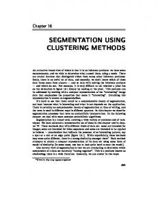
(a)
(b)
Figure 1.4: A fast object (object 1) and a slow object (object 2) move against a static background. (a) If the threshold τ is dependent upon velocity, then the slowly moving object is never detected because ∆x2 /∆t2 < τ . (b) In contrast, a fixed reference frame enables both objects to be detected independently of their speed, as soon as enough image evidence accumulates (time t1 for object 1 and t2 for object 2). able to distinguish between two common cases. First, the pixels in a region may not be moving coherently due to the presence of multiple objects occupying the region, in which case the group should be split. Secondly, the motion divergence may be due to unmodeled effects in the underlying motion model, in which case the reference frame should be updated. Based on the study of the previous work and the above discussion, several common themes emerge regarding limitations of the existing motion segmentation approaches. First, batch processing is quiet common, with many approaches operating either on two images at a time or on a spatio-temporal volume containing a fixed number of images. In the case of multiple frames, the motion of the object is often considered to be constant or slowly changing throughout the sequence of frames under consideration to simplify the integration of information over time. Secondly, the techniques are usually limited to a small time window in which the motion of all of the objects is expected to be well behaved. Additionally, it is generally the case that the focus of the research is not upon computationally efficient algorithms, leading in some cases to techniques that require orders of magnitude
9
more than is available in real-time applications. Finally, some of the techniques are limited to a small number of objects (two or three), due to either the computational burden or more fundamental aspects of the algorithm.
1.3 Thesis Outline The main goal of the work presented in this thesis is to propose an approach for motion segmentation that is able to handle long image sequences with an arbitrary number of objects, is automatic with a few user defined parameters, and is computationally efficient. A mixture model framework is employed for the purpose of segmentation, where it is assumed that the individual moving regions in an image sequence follow parametric motion models and the overall motion in the sequence is the resultant mixture of these individual models. To describe a mixture, it is necessary to specify the kind of motion each region undergoes (nature of the parameters of the model), a set of observable data elements, and a procedure to learn the parameters of each of the models which in turn guide the segmentation. The observed data in this work are the sparse motion trajectories that are obtained by detection and tracking of point features in a joint manner through the consecutive frames of the sequence. Each moving image region is composed of sparse points whose trajectories follow an affine motion model. To obtain a suitable segmentation, parameters of these affine motion models are learned using a novel procedure based on Expectation Maximization (EM). The long term handling of the feature groups is done by maintaining existing groups (splitting them if required), or addition of a new group altogether. One of the secondary goals of this work is to explore a special motion model tailored for handling articulated human motion. Since articulated motion cannot be completely described by any conventional motion model, special models are required for its description. Hence, the goal is to learn the various pose and viewpoint configuration of human gait and use them 10
for segmentation and pose estimation of articulated human motion. Another goal of the work presented in this thesis is to describe the use of mixture models for segmentation of natural images as well as a special application involving iris image segmentation. The thesis is organized in the following manner. Chapter 2 describes the various mixture models, notably the spatially variant mixture models in the context of image segmentation. A general description of the EM algorithm for parameter estimation is given. A greedy spatially variant mixture model, an extension of the existing spatially variant mixture model, is proposed that overcomes some of the limitations of the existing models with respect to the initialization and computational efficiency. Implementation of the various mixture models described in this chapter is shown for segmentation of natural images. Image segmentation, being a more intuitive and simpler to understand application of mixture models, is chosen here to demonstrate the effectiveness of the proposed greedy spatially variant mixture model. Another reason for demonstrating the mixture model algorithms using image segmentation is that many of the previous approaches describe mixture models in the context of image segmentation. Chapters 3 and 4 form the bulk of the proposed motion segmentation approach. Chapter 3 describes tracking of point features in image sequences. Topics covered in this chapter include the basics of motion estimation, detection and tracking of point features, and a joint feature tracking algorithm that, as the name suggests, tracks point features in a joint fashion instead of tracking them independently as is done by the conventional feature tracking algorithms. This joint feature tracking approach was presented at the IEEE Conference Computer Vision and Pattern Recognition (CVPR), 2008 [9]. In joint feature tracking, the neighboring feature points influence the trajectory of a feature and this property can be used to track features reliably in places with less or repetitive texture. The motion vectors obtained from point feature trajectories are used as the input data for the motion segmentation algorithm described in the next chapter. 11
Chapter 4 begins by describing how to adapt the greedy spatially variant mixture model introduced in Chapter 2 for motion segmentation. Specifically, an affine motion model and a neighborhood computing criterion in the case of sparse features is described. Following the description of the algorithm, experimental results are demonstrated on various sequences. The motion segmentation algorithm performs in real time on a standard computer, handles an arbitrary number of groups, and is demonstrated on several challenging sequences involving independently moving objects, occlusion, and parallax effects. The number of groups is determined automatically and dynamically as objects move relative to one another and as they enter and leave the scene. The primary parameter of the algorithm is a threshold that captures the amount of evidence (in terms of motion variation) needed to decide that features belong to different groups. A part of this algorithm was described in the paper published in IEEE Transactions of Systems, Man, and Cybernetics, 2008 [80]. Segmentation using articulated human motion models is described in Chapter 5. The idea is to learn articulated motion models corresponding to various pose and view angle configuration using 3D motion capture (mocap) data which is obtained from the trajectories of the markers attached to the various body parts. A single gait cycle is quantized into a fixed number of pose configurations as is the 360◦ of field of view. Motion vectors of the markers in 2D can now be obtained for each pose and view angle and their discriminative ability is captured by a spatially salient motion descriptor. These descriptors are used for segmentation of articulated human motion and pose estimation. The advantage of this approach is that it is purely motion based and hence can be applied to scenes where extractions of appearance information is difficult. Chapter 6 revisits the problem of image segmentation in the context of segmentation of iris images. This application differs from the generic image segmentation presented in Chapter 2 due to the fact that a lot of a priori information is available in the case of iris images as compared to generic natural images. The number of components as well as the 12
shape of the iris and pupil are known a priori, thus leads to a much simplified formulation of the segmentation problem. Texture and image intensity information is utilized along with the shape information for segmentation of iris regions. Results are demonstrated on non-ideal iris images that suffer from illumination effects, occlusion and in and out of plane rotation. The iris segmentation approach was presented at the CVPR Workshop on Biometrics, 2008 [81]. Conclusions, contributions of the thesis and some potential directions for future work are presented in Chapter 7.
13
Chapter 2 Mixture Models for Segmentation Mixture models, which are extensively used in segmentation, form an integral part of the motion segmentation algorithm that will be presented in Chapter 4. This chapter gives a general description of mixture models, their various formulations, the methods of learning the mixture parameters, and their use in segmentation. Beginning with the definition of a Finite Mixture Model (FMM) and the Expectation-Maximization (EM) algorithm for parameter estimation, this chapter goes on to describe the Spatially Variant Finite Mixture Models (SVFMMs) that can produce a smoother labeling compared with FMMs. Several limitations of SVFMMs are discussed which motivate a new approach based on iterative region growing that improves upon the existing SVFMM framework. Termed as Spatially Constrained Finite Mixture Model (SCFMM), the effectiveness of the new approach is demonstrated vis-` a-vis the existing mixture models in the context of image segmentation. The chief purpose of this chapter is to provide a theoretical backing to our region growing approach by connecting it with the spatially variant mixture models and the EM algorithm. The reader may wish to skip the mathematical details of the mixture models in this chapter on first reading, since our motion segmentation algorithm may be understood without these details. 14
Most previous work in mixture models and EM is aimed at image segmentation. In [21], the EM algorithm is used for learning component density parameters of an FMM for image segmentation was described . The SVFMMs were first proposed in [86] for image segmentation, and its various extensions were presented in subsequent works [76, 11, 33, 88] that introduce different prior models and different ways of solving for the parameter estimates. While many approaches rely on Expectation Maximization for maximizing the likelihood, an approach presented in [117] uses a combination of EM and graph cuts (originally proposed in [17]) for energy minimization.
2.1 Finite Mixture Models Clustering or labeling problems are common in computer vision where an observed data element has to be classified as belonging to one of K classes (also referred to as components, groups, or clusters), K being a positive integer. For example, the objective of image segmentation is to assign a label to each pixel from a set of finite labels based on some image property. In addition to assigning the labels, it is also necessary to estimate the overall properties of the pixels having the same labels (estimate the class parameters). Hence, if each class follows a particular probability density function, then any pixel in the image can be considered as a sample drawn from the mixture of the individual class densities. Finite mixture models (FMM) provide a suitable framework to formulate such labeling problems, where mathematical techniques are already established for estimating the labels and the class parameters [74]. A density function describing a finite mixture model with K components is given by: g(x(i) ) =
K X
πj φ(x(i) ; θj ),
j=1
15
(2.1)
where x(i) is the ith observation (a random variable or vector), φ(x(i) ; θj ) is the density function of the jth component with θj parameters, and πj is the corresponding mixing weight such that
PK
j=1
πj = 1, and πj ≥ 0, j = 1, . . . , K. The mixing weight for a component can
be considered as the prior probability of drawing a sample from that component. A Gaussian mixture model (GMM) is a special case of FMM where individual component densities are Gaussian, i.e., −(x(i)
1
exp φ(x(i) ; µj , σj ) = q 2πσj2
− µ j )2 , 2σj2
(2.2)
where µj and σj are the mean and the standard deviation of the jth Gaussian density (paD
E
rameters of the Gaussian density function, θj = µj , σj ). Figure 2.1 shows an example of a grayscale image whose intensities can be modeled as a mixture of four 1D Gaussian densities. The individual component densities observed in many of the computer vision problems such as segmentation are often approximated by Gaussian densities due to which GMMs are the commonly used mixture model. Learning the mixture constitutes estimating the parameters θ1 , . . . , θK and the mixing weights π1 , . . . , πK for the K components. There are two basic ways in which the parameters (and the mixing weights) can be estimated: maximum-likelihood (ML) or maximum a posteriori (MAP). These estimates can be found using algorithms such as Expectation-Maximization (EM) which is most commonly used to determine the ML or MAP estimates of the parameters of a mixture density.
16
Figure 2.1: An example of a Gaussian mixture model. LEFT: A grayscale image. RIGHT: Mixture of four Gaussian components from which the pixels of the image on the left are drawn as random samples.
2.2 Parameter Estimation Using Expectation Maximization (EM) Parameter estimation is based on the observed data. Assuming that the amount of observable data is finite and discrete, let x(i) denote the ith data sample from a total of N D
E
samples, and let X = x(1) , . . . , x(N) be the entire data set. For the sake of convenience, the parameters of individual component densities and their corresponding mixing weights for the mixture model given in equation (2.1) are represented in a combined fashion by Θ = hπ1 , θ1 , . . . , πK , θK i, such that Θj = hπj , θj i.
2.2.1 MAP Formulation MAP is also known as Bayesian formulation as it is based on Bayes’ rule. The parameters, that are to be estimated, are assumed to follow a known (a priori) distribution. From Bayes’ rule, the a posteriori probability density function of the parameters of the jth
17
component, Θj , given the ith data sample x(i) is g(Θj ; x(i) ) =
πj φ(x(i) ; θj )g(Θj ) , g(x(i) )
(2.3)
where φ(x(i) ; θj ) is the density function of the jth component, πj is the prior probability of that component, g(Θj ) is the prior density on the parameters of the jth component, and g(x(i) ) is a constant value that depends on the observed data. For the entire mixture (all K components) given a single data element it can be written as
(i)
g(Θ; x ) =
K X j=1
πj φ(x(i) ; θj )g(Θj ) . g(x(i) ) !
(2.4)
Assuming that the N data samples are independent, equation (2.4) can be modified to
(1)
(N)
g(Θ; X ) = g(Θ; x , . . . , x
(1)
(N)
) = g(Θ; x ), . . . , g(Θ; x
) =
N Y
g(Θ; x(i) ). (2.5)
i=1
From equations (2.4) and (2.5), the a posterior probability of the set of parameters given the entire data is g(Θ; X ) =
K N X Y
i=1 j=1
πj φ(x(i) ; θj )g(Θj ) . g(x(i) )
(2.6)
The MAP estimate of the parameter set can now be obtained by maximizing g(Θ; X ), i.e., ˆ MAP = arg max {g(Θ; X )} . Θ Θ
(2.7)
Usually, instead of maximizing the actual density term, its log is maximized in order to simplify the calculations. Also, since the denominator of equation 2.6 is a scaling factor, it can be conveniently ignored for maximization operation, leading to the MAP estimate
18
equation ˆ MAP = arg max Θ Θ
N X K X
log{πj φ(x(i) ; θj )g(Θj )} .
(2.8)
i=1 j=1
Differentiating the above equation, equating it to zero and solving it further yields MAP estimate of parameters.
2.2.2 ML Formulation There are many situations when the prior probability distribution of the parameters P(Θ) is unknown. A convenient way is to assume that Θ is uniformly distributed and is equally likely to take on all possible values in the parameter space. Hence, the prior probability density function g(Θj ) in equation (2.3) can be eliminated. Since the denominator g(x(i) ) in equation (2.6) can be ignored, maximizing the a posteriori probability density function is equivalent to maximizing the likelihood function. The likelihood function is given by L(Θ) =
N X K Y
πj φ(x(i) ; θj ).
(2.9)
i=1 j=1
Maximizing the likelihood function in equation (2.9) leads to the maximum likelihood (ML) estimate of the parameters N X K Y
ˆ ML = arg max Θ Θ
i=1 j=1
πj φ(x(i) ; θj ) .
(2.10)
As in the case of MAP estimation, log of the likelihood function can be maximized instead of the above equation so that ˆ ML = arg max log Θ Θ
N X K Y
i=1 j=1
πj φ(x(i) ; θj )
= arg max
19
Θ
N X K X
i=1 j=1
n
log πj φ(x(i) ; θj )
o
.
(2.11)
The following two sections describe an algorithm for ML estimation of the parameters of the mixture model.
2.2.3 Complete Data Log Likelihood Function Revisiting the initial labeling problem, it can be seen that the ML or MAP formulations presented above do not explicitly consider pixel labels. They only consider the observed data X , which is termed as incomplete data [86, 85]. Usually, the pixel labels are represented as hidden or missing variables on which the observed data is conditioned. Let c(i) be a K dimensional vector associated with the ith observed data element x(i) , such that its jth element is (i) cj
=
1
if x(i) ∈ jth component
.
(2.12)
0 otherwise
The vector c(i) is a K dimensional binary indicator vector. There are N such indicator vectors, one corresponding to each observed data element, and they are used to indicate which class the data elements belong to. It is assumed that x(i) belongs to only one class as seen from equation (2.12). Observed data X = {x(1) , . . . , x(N) } along with the corresponding binary indicator vectors C = {c(1) , . . . , c(N) }, are called complete data [14, 86] and can be represented as y(i) = {x(i) , c(i) } or for the entire set, Y = hX , Ci. Introduction of the indicator vectors to make the data “complete” allows for a tractable solution for the EM update equations (described in next section). The density function for the complete data likelihood is given by
g(Y; Θ) =
N Y K � Y
i=1 j=1
(i)
πj φ(x ; θj )
�c(i) j
.
(2.13)
Details of the derivation of the density function in (2.13) can be found in Appendix A.1. The likelihood function, defined in the previous section over incomplete data can be modi-
20
fied to represent complete data as
Lc (Θ) = log {g(X , C | Θ)} = log {g(Y | Θ)} .
(2.14)
This modified likelihood function representing the complete data is iteratively maximized using the EM algorithm to find the maximum-likelihood estimates of the parameters.
2.2.4
Expectation Maximization Algorithm The Expectation-Maximization (EM) algorithm consists of two steps. In the expec-
tation step or E step, the hidden variables are estimated using the current estimates of the parameters of the component densities. In the maximization or M step, the likelihood function is maximized. The algorithm requires an initial estimates of the parameters. Hence, ML estimates of the parameters are given by ˆ ML = arg max {E[log(g(X , C | Θ))]} , Θ
(2.15)
Θ
where E(.) is the conditional expectation function. The EM algorithm can now be described. From equations (2.13), (2.14), and (2.15) the E step can be written as
E [Lc (Θ)] =
N X K X i=1 j=1
�
(i)
�
�
�
E cj ; x(i) , Θ log πj φ(x(i) ; θj ) .
(2.16)
(i)
Since the elements cj of the binary indicator vectors can be assigned to either 1 or 0, �
(i)
(i)
�
(i)
E cj ; x(i) , Θ = P(cj = 1 | x(i) , Θ). Bayes’ rule is applied to P(cj = 1 | x(i) , Θ) to obtain
(i)
(i) P(cj
(i)
P(x(i) | cj = 1, Θ)P(cj = 1 | Θ) = 1 | x , Θ) = P(x(i) | Θ) (i)
21
(2.17)
E
(i) cj ;
�
πj φ(x(i) ; θj ) x , Θ = PK = wj (x(i) ; Θ) (i) j=1 πj φ(x ; θj ) �
(i)
(2.18)
This is nothing but a Bayes’ classifier. Hence, to assign the class labels to the corresponding data elements, maximum probability value obtained from the Bayes’ classifier can be used (see Figure 2.2). Explanation of EM algorithm involves the use of the likelihood funcˆ that would maximize tion of equation (2.16) and finding the estimate of the parameters Θ ˆ (t) be the estimated parameters at the tth this function as shown in equation (2.15). Let Θ iteration. The E step finds the expectation of the log-likelihood function and for the (t +1)th iteration given by N X K X
ˆ (t) ) = Q(Θ; Θ
�
�
ˆ (t) )log πj φ(x(i) ; θj ) , wj (x(i) ; Θ
i=1 j=1
(t) (t) πˆj φ(x(i) ; θˆj ) (t) ˆ where wj (x ; Θ ) = PK (t) (t) ˆj φ(x(i) ; θˆj ) j=1 π (i)
(2.19)
(2.20)
and π ˆj and θˆj are the estimates of πj and θj respectively obtained at the tth iteration. The maximization step now involves finding ˆ (t+1) = arg max Q(Θ; Θ ˆ (t) ). Θ Θ
(2.21)
Since the mixing weights and the density parameters are independent of each other, their expression can be determined separately. The update equation for the mixing weights is given by (t+1)
πj
=
N 1X ˆ (t) ). wj (x(i) ; Θ N i=1
(2.22)
For derivation of (2.22), please refer to Appendix A.2. Assuming that the individual component densities are Gaussian in nature as shown in equation (2.2), the objective is to find the expressions for the mean µj and the standard deviation σj . For finding the expression 22
Figure 2.2: Assigning labels to the data for an FMM. LEFT: Each data element is rep(i) resented by a set of weights wj corresponding to the components of the mixture model. CENTER : The mixing weights πj for each component are obtained by summing up and (i) normalizing the wj for all the data elements. RIGHT: The final label is assigned based on the component that has the maximum weight for a given data element. for the class mean and standard deviation the log-likelihood function from equation (2.16) is differentiated with respect to µj and σj and equated to zero. The final update equations for the mean and standard deviation are given by µ(t+1) j
PN
ˆ (t) )x(i) wj (x(i) ; Θ . (i) ˆ (t) i=1 wj (x ; Θ )
i=1 = P N
(2.23)
Similarly, the expression for the standard deviation update is given by:
(t+1) σj
=
v uP u N w (x(i) ; u i=1 j t P N i=1
ˆ (t) )(x(i) − µ(t+1) )2 Θ j . (i) (t) ˆ wj (x ; Θ )
(2.24)
The E and M steps continue until convergence i.e., until L(Θ(t+1) ) > L(Θt ). EM is guaranteed to converge to some local minimum [32]. Appendix A.2 provides the details of derivation of the expressions for the class mean and standard deviation.
23
2.2.5 Limitations of the Finite Mixture Models Even though FMMs provide an effective framework to mathematically formulate and solve a variety of clustering problems, some major limitations exist that limit their use in segmentation or labeling problems. 1. Direct estimation of data labels not possible: Classification of the data in a FMM is performed using the Bayes’ classifier described in equation (2.18) which determines the maximum a-posteriori probability of an element of the data belonging to a particular class based on the mixing weights (prior) and the component densities (likelihood). This is a soft classification, i.e., for each data element, there exists a set of probabilities belonging to each of the components and for classification, the maximum value amongst them is chosen. Hence, the FMMs do not allow for the direct estimation of the data labels, and an indirect approach has to be utilized. 2. Absence of spatial correlation between the observations: While arriving at a likelihood function to be maximized in equation (2.9), one of the key assumptions was that of the statistical independence of the observed data. This assumption, while simplifying the derivation to obtain and maximize the likelihood function, affects the ability of classification of the observed data in cases where spatial saliency of the data is important. For example, in the case of image segmentation, the nearby pixels are more likely to have the same grayscale intensity or color. FMMs cannot utilize such spatial information for classification, unless the spatial coordinates are part of the data vector. Even then, such a segmentation may have regions that are not spatially constrained (regions produced may be disconnected), and such an approach imposes elliptical model which does not accurately represent arbitrarily shaped regions. An improved model is required that can take into account the spatial information for classification in such a way that the labeling appears smooth. 24
2.3 Spatially Variant Finite Mixture Models An SVFMM can be considered as a more generalized form of an FMM. The main difference between the two models is that in the SVFMM, instead of the mixing weights, each data element has label probabilities. As previously defined, there are K components in a FMM and mixing weights corresponding to each component is represented by πj such that
PK
j=1
πj = 1 and πj > 0. In a SVFMM, the mixing weights become label probabilities,
i.e., a K dimensional weight vector for each observation, whose elements describe the probability of the observation belonging to the corresponding components. Let π (i) be the label (i)
probability vector corresponding to the ith data element, and πj be its jth component, then (i)
πj represents the probability of the ith data element belonging to the jth component. There are N number of such K dimensional weight vectors with the conditions that (i)
PK
j=1
(i)
πj = 1
and πj > 0, ∀ i = 1, . . . , N. The density function for the ith observation can be defined as (i)
g(x ; π
(1)
...π
(N)
, θ1 . . . θK ) =
K X
(i)
πj φ(x(i) ; θj ).
(2.25)
j=1
Considering the observed data to be statistically independent, the conditional density for the entire set of observations is given as
g(X ; π
(1)
...π
(N)
, θ1 . . . θK ) =
N X K Y
(i)
πj φ(x(i) ; θj ).
(2.26)
i=1 j=1
It can be seen from the above equation that there are some differences in the parameters on which the data is conditioned in the SVFMM as compared to the FMM. Here the set D
E
of parameters can be represented as Θ = π (1) . . . π(N) , θ1 , . . . , θK . Hence, the number of parameters to be estimated in the case of an SVFMM is comparable to the amount of observed data (N × K label probabilities and K component density parameter vectors) whereas in the case of FMM, this value is invariant of the amount of data (K mixing weights 25
and parameter vectors). EM algorithm can be used to find either the ML or MAP estimates of the parameters of an SVFMM.
2.3.1 ML-SVFMM ML estimation of parameters for an SVFMM is similar to that of an FMM except in one key area which will be described momentarily. An interesting property of the label (i)
probabilities πj
is that their ML estimates converge to either 0 or 1, thus enforcing a
binary labeling (for details, see [86]). The expressions for the label probabilities and the parameters of the component densities (assuming Gaussian) for the (t + 1)th iteration are given by (i)(t+1)
πj
where
�
(i) wj
� � 1 (i) (t) , = P � �(t) wj (i) K w j j=1
�(t)
�
� (i) (t)
πj
(2.27)
φ(x(i) ; (θj )(t) )
= P � �(t) , (i) K (i) ; (θ )(t) ) φ(x π j j j=1
� � 1 (i) (t) (i) x , w µ(t+1) = j j PK � (i) �(t) j=1 wj
(2.28)
(2.29)
N � �2 � � X 1 (i) (t) x(i) − µ(t+1) . wj (σj2 )(t+1) = P � �(t) j (i) N i=1 w j i=1
(2.30)
Equations (2.27) - (2.30) for the ML estimation of the SVFMM parameters are very similar to the corresponding equations of the FMMs with one essential difference. In the case of ML-SVFMM, the label probabilities of a data element for the next iteration are the �
� (i) (t+1)
weights computed in the current iteration: πj
�
� (i) (t)
= wj
. Unlike the FMMs, in
ML-SVFMM the pdfs over the data elements are not summed up and normalized to obtain one prior probability per component. Instead, each data element retains its pdf over the components which acts as a prior for the next iteration. Because of this difference, the
26
labeling becomes spatially variant. Since the label probabilities are directly estimated, SVFMM addresses the first concern regarding FMMs stated in section 2.2.5, but it does not address the limitation of spatial continuity of the labels (because there is no interaction between the neighboring labels) since in ML estimation the prior on the parameters is assumed to be uniform. To effectively utilize the SVFMM framework, a suitable prior for the label probabilities is required that enforces spatial continuity on the estimated labels. This is the motivation for performing MAP estimation.
2.3.2 MAP-SVFMM Maximum a posteriori estimation of parameters of an SVFMM can incorporate spatial information in the observed data. This is done by choosing a suitable prior probability density function for the parameters to be estimated. For a SVFMM, the set of parameters E
D
to be estimated is given by Θ = π (1) . . . π (N) , θ1 , . . . , θK , and therefore the prior density (i)
function is given by g(Θ) = g(π (1) . . . π (N) , θ1 , . . . , θK ). Since the label probabilities {πj }, and the component density parameters {θj } are independent, the prior density function can be written as g(Θ) = g(π (1) . . . π (N) )g(θ1 , . . . , θK ). The a posteriori density function is given by
g(π (1) . . . π (N) , θ1 , . . . , θK ; X ) ∝ g(X ; π (1) . . . π (N) , θ1 , . . . , θK )g(π (1) . . . π (N) , θ1 , . . . , θK ) (2.31) g(π (1) . . . π (N) , θ1 , . . . , θK ; X ) ∝ g(X ; π (1) . . . π (N) , θ1 , . . . , θK )g(π (1) . . . π (N) )g(θ1 , . . . , θK ) (2.32) While choosing a prior density for Θ, the component parameters can be assumed to follow a uniform distribution thus leaving only the label probabilities to be selected. It is usually the case that in typical labeling applications only local interactions of the data elements are important. By local interactions, it is meant that the label assigned to a data 27
element is only affected by the labels of its immediate neighbors. This leads toward a Markov Random Field (MRF) assumption on the label probabilities. Three key aspects of representing the local interactions in the observed data using MRF are: a method to impose spatial connectivity, a parameter that defines the local neighborhood and a function that defines the strength of the local interactions. These requirements are met by treating the problem as a graph with the vertices representing the data and the edges modeling the connections between the neighboring data elements. The size of the neighborhood is determined by the order of the clique. In an undirected graph, a clique of order n is the set of n vertices that are connected to each other. Gibbs density function is a commonly used function to represent the MRF based label prior density and is defined as g(π(1) . . . π (N) ) =
h i 1 exp −U(π (1) . . . π (N) ) , Zβ
(2.33)
where U(π (1) . . . π (N) ) = β
X
Vn (π (1) . . . π (N) )
(2.34)
n∈M
and β and Zβ are constants, Vn (.) is the clique potential function that determines the strength of interaction between the clique vertices and M represents the set of all possible cliques in the observed data. The parameter β regulates the overall effect of the prior probability term on the label assignment process, and a high value of β signifies the increased influence of neighboring label probability terms on the current data element, creating an effect similar to spatial smoothing. The clique potential function is chosen in such a way that it assigns higher label probability to a data element if its neighbors have been assigned the same labels. So in the local neighborhood N (i) of the ith data member, the clique potential function for the nth
28
Figure 2.3: Markov Random Field with 2nd order cliques for a 4-connected and 8-connected neighborhood. order clique is defined as
X
Vn (π (1) . . . π (N) ) =
n∈M
X
K � X
(i,m)∈N (i) j=1
π (i) − π(m)
�2
.
(2.35)
A commonly used clique order is two, which leads to the pairwise interaction of data elements. In the case of images, the local neighborhood is usually defined as 4-connected or 8-connected (see Figure 2.3). From equations (2.33), (2.35), an expression for the prior probability density is obtained that can be used in equation (2.32) to solve for the MAP estimation of the parameters. Details of the procedure adopted to arrive at the parameter estimates can be found in [86].
2.4 A Spatially Constrained Finite Mixture Model (SCFMM) The SVFMM based labeling is supposed to generate smooth labels, but there is still a possibility that spatially disjoint regions may be assigned the same labels. This property 29
is undesirable especially if a large number of small regions are segmented in the interior of a big region. In order to rectify this effect the segmentation has to be constrained to produce a labeling which follows the spatial continuity of the data elements. Additionally, two chief limitations of the EM algorithm for parameter estimation of the SVFMMs are related to its initialization and its computational cost. The number of components may not be known a priori in many cases. Consequently, the EM algorithm for solving for SVFMMs has to use a value of K predefined by the user or has to resort to using a separate initialization routine. Similarly, initialization of the component density parameters is not a trivial task given that they have a large impact on the segmentation outcome. For Gaussian component densities, if the initialization is not close to the actual mean, then the EM algorithm can get stuck into local minima and not converge to the desired location. More importantly, the variance initialization also has to be optimum; where a large value can lead the algorithm astray, or too small a value can make the algorithm susceptible to noise. Initialization also determines the amount of time it takes to reach convergence. Generally, algorithms that are based on spatial smoothing like MAP-SVFMM tend to be slow as they process the neighborhood of each pixel for multiple iterations. Due to these reasons, an approach is required that is fast and does not need explicit initialization in terms of number of components. The spatially constrained finite mixture model (SCFMM)1 is a variation of the SVFMM, where the emphasis is on assigning spatially connected labels which can be computed by a greedy EM algorithm. Although the term greedy EM was introduced in [106], our algorithm is agglomerative as opposed to the divisive nature of the previous algorithm. The algorithm can automatically determine the number of groups and is also computationally efficient as compared to the standard EM algorithm used for solving MAP-SVFMM. The greedy EM is inspired from the region growing algorithm. In region growing algo1
Our use of the term spatially constrained should not be confused with that of [76], where the term describes a variation of the SVFMM [86] that smooths the label probabilities across the pixels but does not constrain the connectivity of the segmented region.
30
rithm, starting from a seed location, the neighboring pixels are incrementally accumulated if they satisfy a particular condition. This condition is problem dependent and could be, for example, to include all pixels with grayscale values below a certain threshold. The region growing stops when no more pixels can be added to the already accumulated ones. Then another location is chosen and the growing procedure is repeated all over again. This region growing technique has some interesting properties. First, it does not need to know the total number of regions in the given data. In fact, the number of segmented regions is the output of the algorithm. The starting locations can be chosen at random or deterministically, and it is not totally unreasonable to assume that the segmentation output is somewhat independent of the choice of the seed points although this is not guaranteed. Another property is that the component parameters are initialized and learned on the fly as the processing proceeds. Also, region growing has strong spatial connotations. Since region growing is done locally, i.e., by accumulating immediate neighbors, there is no risk of labeling spatially disconnected regions with the same label. This property points toward the idea of the algorithm being spatially constrained. Finally, the algorithm can be implemented in a very efficient manner. One limitation of such a region growing approach is that being a local process, it can ignore the higher level information which can lead to generation of undesirable regions due to noise. The criterion for inclusion of neighboring pixels has to carefully selected, otherwise there is a risk of a region growing too big or too small (overor under-segmentation). To learn the parameters, the region growing algorithm can be run repeatedly for a single region until a stable set of pixels are obtained. The properties of the set can be updated at each iteration to refine the inclusion criterion. This is similar in spirit to the parameter estimation process in other mixture models using the EM algorithm, especially a greedy EM algorithm where the clusters are automatically determined at the end. Consider an example of iterative region growing. Starting from a random location in the image, 31
the region parameters can be initialized over a small neighborhood. At the end of the first iteration, the region parameters and a new mean location are obtained. This new location, now becomes the starting location and the region parameters become the initial estimates for the second iteration. Progressively, mean and variance values are refined, and the algorithm converges to a set of parameters (or a particular labeling) that do not change after subsequent growing iterations. The SCFMM and the greedy EM algorithm can now be formulated. Assuming that the observed image data is independent of each other given the parameters, the probability of describing the entire observed data given the set of parameters can be written as
P(X , C | Θ) = D
N X K Y
i=1 j=1
(i)
(i)
(i)
P(x(i) | cj , Θ)P(cj | Θ), (i)
E
(2.36)
where C = {c(1) , . . . , c(N) }; c(i) = c1 , . . . , cK , are the binary labels on the pixels similar (1)
(N)
to (2.12). For the jth component the data independence assumption means P(cj , . . . , cj Θ) =
QN
i=1
|
(i)
P(cj | Θ). A more realistic formulation that is in accordance with the proposed
SCFMM would take the spatial continuity of the regions in account. For the ith pixel, its (i)
label Cj depends on its parents i.e., the pixel that included the ith pixel in the group. This way, the pixels of region growing can be arranged in a chain starting from the seed location to the current pixel yielding (1)
(N)
P(cj , . . . , cj
| Θ) = =
N Y
i=1 N Y
i=1
(i−1)
on the account of cj
(i)
(i−1)
P(cj | cj (i)
, Θ)
(i−1)
P(cj | Θ)cj
,
(i)
also being a binary variable. Extending this result to 2D, let ǫj be
a binary variable for the jth component whose value is 1 if and only if there exists a path (according to a predefined neighborhood) from the ith pixel to the seed location such that 32
(l)
cj = 1 for all pixels x(l) along the path. As actual labels are unavailable, an estimate of (i)
(i)
(l)
ǫj given by ǫˆj is used, which is set to one if P(cj | Θ) > pτ for all the pixels along the path, where pτ is a predefined threshold. This leads to a greedy EM like algorithm with the following update equations
�
(i)
πj
�(t+1)
�
� (i) (t)
πj
(t)
�
� (i) (t)
φ(x(i) ; θj ) ǫˆj
= P � �(t) � �(t) (i) (t) (i) K φ(x(i) ; θl ) ˆǫl l=1 πl (i) ˆǫj
=
�
(l) min πj l
�
> pτ
N � � X 1 (i) (t) (i) x µ(t+1) = π � � j j PN (i) (t) i=1 π j i=1
�
σj2
�(t+1)
N � �2 � � X 1 (i) (t) = P � �(t) x(i) − µj(t+1) πj (i) N i=1 i=1 πj
(2.37)
(2.38) (2.39)
(2.40)
2.5 Application of Mixture Models for Image Segmentation The use of the various mixture models proposed in the previous sections for image segmentation is now demonstrated.
2.5.1 Implementation Details A general clustering problem using various mixture models described in the previous sections involves answering the following questions: • What is the nature of the data? • How many components are present in the mixture model? 33
• What are the mixing weights (or label probabilities) of the components? • What density functions do the components follow and what are the parameters? • What is the prior on the parameters? • How is the system solved to obtain the parameter estimates and classification labels? For the problem of image segmentation, the data to be clustered can be the pixel values or any other quantity derived from the image (such as texture). Furthermore, the observed image data is considered to be sampled from a mixture of probability density functions. The nature of such mixture models with regard to the kind of component densities and their parameters is assumed to be known beforehand. This helps in establishing the objective for any formal procedure used to obtain a solution, i.e., to estimate the parameters and the mixing weights. In this section, segmentation based on image color or grayscale intensities is described, and hence the data is either scalar (grayscale images) or a vector (3 × 1 color vector). Let I be the input image with N pixels, and let x(i) be its value at the ith pixel. The important thing to note here is that the pixel value x(i) is an observed quantity because an image is assumed to be corrupted by Gaussian noise of variance ση2 . The component densities are assumed to be Gaussian and the dimensionality of their corresponding parameters, the component means and the variances, depend on x(i) . The goal is to obtain a labeled image L, such that L(i) = j; j = 1, . . . , K. The key factor that is mostly implementation dependent is the number of components K or labels. This has to be supplied externally and all the parameter estimation expressions for a given mixture model depend on the value of K. The parameter estimates are obtained iteratively by the maximization of likelihood (or minimization of energy) using the EM algorithm. For the mixture models introduced in the previous sections, the algorithms EM-FMM, EM-ML-SVFMM and EM-MAP-SVFMM describe the parameter estimation and the labeling process. 34
Algorithms EM-FMM, EM-ML-SVFMM are shown in Figures 2.4, and 2.5, respectively and are relatively straightforward to understand and implement as compared to the EM-MAP-SVFMM. This is because assumption of uniform prior on the parameters which simplifies the likelihood function. It can be solved to obtain expressions for the values of mixing weights (or label probabilities) and means and the variances which are updated for every iteration until convergence is achieved. The MAP-SVFMM on the other hand assumes that the pixel label probabilities follow the MRF model. This leads to a likelihood function with additional terms. The label probabilities need to be estimated in a constrained manner, i.e., ensuring that for a pixel the probability values with respect to all labels should sum to unity. The net effect of this is that additional steps need to be performed for constrained optimization using techniques like gradient projection. This is shown in steps 2(b) i - vii of the algorithm MAP-SVFMM shown in Figure 2.6. The EM-MAP-SVFMM here is reproduced form [86] where is described in its entirety along with a detailed analysis. Two important aspects of the parameter estimation process using EM are initialization and convergence. EM requires a good initialization to arrive at desired results. Good initialization refers to starting close to the desired or expected parameter estimates. For a FMM or SVFMM with Gaussian component densities, four quantities need to be initialized, namely, the number of components, the mixing weights (FMM) or label probabilities (SVFMM), the component means, and the variances. Initialization is mostly problem dependent. As described earlier, the number of classes K is usually predefined. The mixing weights or the label probabilities are initialized to 1/K, which eliminates bias toward a particular labeling assignment in absence of any a priori information. Initialization of component densities depends on the data and the range of the data can be used to initialize class means. One way to initialize class means is to ensure that they are at equal distances in the data space. Variance of the components can then be some percent of the variance of the entire data. In the EM algorithm, the likelihood is maximized over a period of time, 35
due to which it takes a certain number of iterations to achieve convergence. The number of iterations varies depending upon the initialization of the parameters as well as the nature of the data. EM is guaranteed to converge at some local minimum. The implementation details of the greedy EM are shown in Figure 2.7. For the sake of implementation, some new terms are introduced. The N × 1 vector b is a binary vector that indicates whether a pixel is labeled. The functions N14 (.), N18 (.), N24 (.), and N28 (.) are the neighborhood computing functions. The subscript denotes the pixel distance and the superscript denotes the neighborhood connectedness. So, N18 (i, b) returns all the unlabeled pixels in the 8-connected neighborhood within 1 pixel distance of the ith pixel, while N28(i, b) returns the unlabeled pixels from a larger neighborhood that are used for initialization of mean and variance for the region to be grown. The function N18 (i, L) returns the labels of the neighbors of the ith pixel. xj denotes the centroid or spatial mean of the jth segment which is iteratively computed. Gj is the set of pixels that are assigned the jth label. As it can be seen, the algorithm does not require any preconditions on the number of components. The means and the variances of each of the potential segment are initialized around each new starting point as the algorithm proceeds. The two important parameters to be set are: i) pτ , the condition of inclusion of a pixel in the current region, and ii) nmin , the minimum number of pixels in a group for it to be declared valid. This limits over-segmentation in case of noise in the image.
2.5.2 Experimental Results Experimental results of the EM-FMM, EM-ML-SVFMM, EM-MAP-SVFMM, and greedyEM-SCFMM algorithms are demonstrated on various test images. Figure 2.8 shows a synthetic image with four different grayscale values 30, 100, 170 and 240. Zero mean Gaussian noise of standard deviation ση = 25 was added to generate the noisy synthetic
36
Algorithm: EM-FMM Input: Noise corrupted grayscale image I with N pixels Output: Labeled image L 1. Initialization: (a) Set a value for number of components, K (b) Set mixing weights, (πj )(0) = 1/K, ∀ j = 1 . . . K
(0)
and variance σj , (c) Set component density parameters, mean µ(0) j and ∀ j = 1 . . . K
(d) Set a value for maximum number of iterations, nitr 2. for t = 1:nitr (a) E STEP i. for i = 1 : N (a) Set x(i) = I(i) (b) for j = 1 : K (i)
• Compute φ(x ;
(t) µj(t) , σj )
=
(t)
1 √ (t) exp 2πσj (t)
−
(x(i) −µj )2 (t)
2(σj )2
(t)
(πj )(t) φ(x(i) ; µj ,σj )
(i) • Compute (wj )(t) = PK
(t) (t) (π )(t) φ(x(i) ; µj ,σj ) j=1 j
(i)
(i)
• Compute Wj = (wj )(t) x(i)
(b) M STEP
i. for j = 1 : K (a) Update mixing weights, (πj )(t+1) = (b) Update class mean,
µ(t+1) j
=
(c) Update class variance,
n
= (i)
(i) (t) i=1 (wj )
PN
PN (i) W PN i=1 (i)j (t) i=1
(t) σj
1 N
PN
(wj )
i=1
o
(i)
h
(t+1)
(wj )(t) x(i) −µj
PN
i=1
(i)
(wj )(t)
i2
3. Update label image, L(i) = arg maxj (wj )(t) , for i = 1, . . . , N Figure 2.4: EM algorithm for parameter estimation in an FMM.
37
!
Algorithm: EM-ML-SVFMM Input: Noise corrupted grayscale image I with N pixels Output: Labeled image L 1. Initialization: (a) Set a value for number of components, K �
� (i) (0)
(b) Set label probabilities, πj
= 1/K, ∀ j = 1 . . . K, and ∀ i = 1 . . . N (0)
(c) Set component density parameters, mean µ(0) j and variance σj , ∀ j = 1...K (d) Set a value for maximum number of iterations, nitr 2. for t = 1:nitr (a) E STEP i. for i = 1 : N (a) Set x(i) = I(i) (b) for j = 1 : K (i)
• Compute φ(x ;
(t) µj(t) , σj )
=
(t)
1 √ (t) exp 2πσj
(i)
(t)
−
(x(i) −µj )2 (t)
2(σj )2
!
(t)
(πj )(t) φ(x(i) ; µj ,σj )
(i) • Compute (wj )(t) = PK
(i)
j=1
(i)
(t)
(t)
(πj )(t) φ(x(i) ; µj ,σj )
(i)
• Compute Wj = (wj )(t) x(i)
(i)
(wj )(t)
(i) • Update label probabilities, (πj )(t+1) = PK
j=1
(i)
(wj )(t)
(b) M - STEP
i. for j = 1 : K (a) Update class mean,
µ(t+1) j
=
PN (i) W PN i=1 (i)j (t) i=1
(t+1)
(b) Update class variance, σj n
(i)
=
(wj )
PN
i=1
o
(i)
h
(t+1)
(wj )(t) x(i) −µj
PN
i=1
(i)
(wj )(t)
i2
3. Update label image, L(i) = arg maxj (πj )(t+1) , for i = 1, . . . , N Figure 2.5: EM algorithm for parameter estimation in an ML-SVFMM. The only difference (i) between this algorithm and the EM-FMM is the use of πj instead of πj . 38
Algorithm: EM-MAP-SVFMM Input: Noise corrupted grayscale image I with N pixels Output: Labeled image L 1. Initialization: same as in algorithms FMM and ML-SVFMM 2. for t = 1:nitr (a) E STEP i. for i = 1 : N (a) Set x(i) = I(i) (t)
(b) Compute φ(x(i) ; µj(t) , σj ) (i)
(c) Compute (wj )(t) (i)
(i)
(d) Compute Wj = (wj )(t) x(i) ii. for i = 1 : N � � � P P (i) (i) (a) s1 = Kj=1 (wj )(t) ln (πj )(t) − β m∈N (i) Vm (π (i) )(t) , π (m) � � � �(t) (t) P φ(x(i) ; θj ) ∂Vm ((π (i) )(t) ,π(m) ) (i) = K (b) qj (i) (i) (t) (t) − β m∈N (i) (i)
P
l=1 (πl
)
; θj )
φ(x
(i)
∂πj
(i)
(c) Evaluate condition ϕ(πj , qj ) = (d) Compute
(Rj,l )(t) =
�
= 0 and 1, if 0, otherwise
π (i) =(π (i) )(t)
(i) qj
(i)
(i)
(i)
0,
(i) πj
0
i. Compute initialization neighborhood nu = N28 (i, b) (k)
ii. πj+1 = 1, k = 1, . . . , | nu | iii. Compute region centroid xj+1 from nu iv. Repeat until xj+1 does not change (a) Compute the nearest pixel, i′ ∈ nu to xj+1 (k)
(b) Set πj+1 = 0, ∀ k 6= i′ (c) Repeat until no more points can be included (l) for each l such that πj+1 = 1 (k) if k ∈ N14 (l, b) && πj+1 == 0 && φ(x(k) ; θj ) > pτ (k) πj+1 = 1 Gj+1 = l (d) Compute µj+1 from Gj+1 2 (e) Compute σj+1 from Gj+1 (f) Compute xj+1 from Gj+1 (i)
v. Set b(i) = max{b(i) , πj+1 }, i = 1, . . . , N vi. Assign labels L(k) = j + 1, ∀ k ∈ Gj+1
vii. if
PN
i=1
(i)
πj+1 ≥ nmin , then j = j + 1
(d) compute ml = N18 (i, L)
(e) compute L(i) = arg minj {φ(x(i) , θj )}, j ∈ ml Figure 2.7: Greedy EM algorithm for parameter estimation in an SCFMM. 40
original
noisy
Figure 2.8: Image used for testing the segmentation output of the various mixture models. LEFT: A synthetic grayscale image composed of 4 different grayscale values. RIGHT: Image on the left corrupted by Gaussian noise with zero mean and a standard deviation of 25. image. The image is constructed in a manner such that spatial coherency of regions is emphasized. Figure 2.9 and 2.10 show the segmentation results of all four algorithms on the noisy synthetic image and the sky image respectively. The value of K was set to 4 and 3 in the synthetic and sky images, respectively, for the EM-FMM, EM-ML-SVFMM, and EM-MAP-SVFMM. The mean and the variance of the components were initialized using the grayscale histogram of the images. For the synthetic and the sky image, the class means were set to {31, 85, 170, 245} and {30, 80, 210} respectively. The class variance was set to 10% of the entire data range. The value of β for EM-MAP-SVFMM was set to 1.0. For the greedyEM-SCFMM algorithm, the value of pτ was 0.005 and nmin was 30 pixels. Segmentation results of greedyEM-SCFMM on various other natural images are shown in Figure 2.11. To quantitatively analyze the results, labeling energy is computed for each algorithm for the synthetic and sky images. Labeling energy measures how close the pixel value is to the class mean for that label as well as how smooth the labeling is with respect to the pixel neighbors. The former term is also known as the data energy while the later is
41
EM-FMM
EM-ML-SVFMM
EM-MAP-SVFMM
greedyEM-SCFMM
Figure 2.9: Output of the EM algorithms EM-FMM, EM-ML-SVFMM, EM-MAP-SVFMM and the greedyEM-SCFMM on the noisy synthetic image.
EM-FMM
EM-ML-SVFMM
EM-MAP-SVFMM
greedyEM-SCFMM
Figure 2.10: Output of the EM algorithms EM-FMM, EM-ML-SVFMM, EM-MAP-SVFMM and the greedyEM-SCFMM on the sky image. 42
input
segmentation
Figure 2.11: Segmentation results of greedyEM-SCFMM on some natural images. The images in the top two rows are segmented using grayscale intensities as the data while those on the bottom two rows use color. The images on the bottom three rows are from the Berkeley Segmentation dataset [73]. 43
also known as the smoothness energy. Formally, the labeling energy can be defined as
Elabel (L, I) = Edata (L, I) + Esmooth (L, I),
where �
� I(i) − µj 1 � − ln 2πσj2 − Edata (L, I) = 2 2σj2 i=1 N X
Esmooth (L, I) =
X
X
i=1N m∈N 4 (i) 1
�2
(2.41)
, withj = L(i), and o
n
exp − (I(i) − I(m))2 δ (L(i), L(m)) ,
(2.42) (2.43)
with δ(.) being the Kronecker delta function given by δ (L(i), L(m))
= 1 , if L(i) = L(m)
0,
.
(2.44)
otherwise
Here the idea is to assign lower penalty (higher energy reduction) if the neighboring pixels of different labels have large differences in their pixel values as compared to those pixels having separate labels but similar values. The reason for choosing this kind of energy function is twofold. First, since the likelihood functions of all the algorithms differ to some extent, this serves as a common energy function to quantify the performance. Second, all the algorithms can now be judged purely on the basis of the labeling output produced. Figure 2.12 shows the energy minimization for the four algorithms tested for the synthetic and the sky images. The greedyEM-SCFMM algorithm, in addition to producing more visually appealing results, also minimizes labeling energy better than the other three. The EM-FMM, EM-ML-SVFMM, and EM-MAP-SVFMM would perform much better with more finer tuning of the parameters. The greedyEM-SCFMM on the other hand does not rely on any explicit initialization. Since it is randomly initialized, plots in Figure 2.13 show the variation in the minimum energy and the number of labels generated for 10 random trials with different starting locations. The plots show the stability of the greedyEM-SCFMM
44
1.15
1.15
labeling energy
labeling energy
SCFMM MAP−SVFMM ML−SVFMM FMM 1.1
1.05
SCFMM MAP−SVFMM ML−SVFMM FMM
1.1
1.05
1
1
2
4
6
8
10
12
14
16
0.95
18
5
10
iterations
15
20
iterations
noisy synthetic image
sky image
Figure 2.12: Plots showing the minimization of labeling energy for the EM-FMM, EM-ML-SVFMM, EM-MAP-SVFMM and the greedyEM-SCFMM algorithms. 20
1.07
18 16
1.05
14
labels
labeling energy
1.06
1.04 1.03
12 10 8
1.02
6
1.01
4 2
1
1
2
3
4
5
6
7
8
9
10
trials
1
2
3
4
5
6
7
8
9
10
trials
Figure 2.13: LEFT: Plot of labeling energy and RIGHT: number of labels detected over 10 random trials of SCFMM on the noisy synthetic image. even though the nature of the algorithm is random. The number of labels varies due to merging of some of the neighboring regions of same intensity values.
2.6 Summary This chapter has described various kinds of mixture models and the EM algorithm used for estimating their parameters. Finite mixture models are not very well suited for
45
spatially salient labeling required in segmentation applications and hence, spatially variant finite mixture models are used for such applications. Concerns regarding the initialization and computational efficiency of the SVFMMs motivate the use of an improved framework for segmentation. Inspired from the region growing approach, this chapter has introduced a novel spatially constrained mixture model with a greedy-EM algorithm for parameter estimation that overcomes the above mentioned limitations of SVFMMs. The effectiveness of the proposed approach is demonstrated using segmentation of images based on color or grayscale values. Later we use the spatially constrained mixture model and the greedy-EM algorithm for motion segmentation. But first, a method to compute image motion has to be described. The next chapter focuses on sparse motion computation in image sequences by tracking feature points.
46
Chapter 3 Point Feature Tracking Image motion can be computed from the sparse feature trajectories obtained by tracking features between two frames. The image motion thus computed can be used for the purpose of motion segmentation. This chapter gives a general overview of the problem of feature tracking and explains how it can be used to compute image motion, with a special emphasis on the Lucas-Kanade method of feature tracking along with its advantages and limitations. The Lucas-Kanade algorithm treats each feature point independently while tracking, but a better assumption is that the motion of a point feature is dependent on its immediate neighbors. Based on this idea, a joint feature tracking algorithm [9] is described that is able to track features more reliably than the Lucas-Kanade algorithm in certain situations such as tracking in less textured regions.
3.1 Motion Estimation Basics Success of a motion segmentation algorithm depends on the accuracy of motion estimation in the given image sequence. Motion in image sequences is observed when a dynamic 3D scene is captured by a camera, i.e., projection of objects moving in a three
47
dimensional world on an image plane gives rise to a motion field. This is different from optical flow, which can be defined as the observed motion of intensity patterns on the image plane. Since changing brightness patterns can also be produced by phenomena that do not involve motion in three dimensions such as specular reflections, the motion field and the optical flow for an image sequence may not be the same. Nevertheless, optical flow is often used to estimate the motion field. One fundamental assumption regarding the nature of the scene is that the moving objects maintain constant intensity profile throughout their motion. This assumption is the famous brightness constancy assumption and forms the basis of all the approaches for estimating optical flow. Let I be an image and I(x(t), y(t), t) denote the intensity of a point projected onto the image at the location (x(t), y(t)) at time t. At a time t + ∆t, the projected point moves to a new location (x(t + ∆t), y(t + ∆t)). According to the brightness constancy assumption, the point has the same intensity at both locations, which means
I(x(t + ∆t), y(t + ∆t), t + ∆t) = I(x, y, t).
Expanding the above equation using Taylor series about the point (x(t), y(t)) and taking the limits, a familiar form of the optical flow equation is obtained which is given by
f (u, v; t) = Ix u + Iy v + It = 0,
(3.1)
where Ix and Iy represent the partial derivatives of the image in x and y directions respectively, It represents the temporal derivative of the image, and u and v are the horizontal and vertical components of the unknown pixel velocity respectively. This classic equation relates the spatial and the temporal derivatives of an image pixel to its velocity vectors. Given a pair of images and their spatial and temporal derivatives, the goal is to determine [u, v]T .
48
Since there is only one equation involving two unknowns, the system is underconstrained, and an unambiguous solution cannot be obtained. This is the well known aperture problem, and herein lies the biggest challenge in estimating the optical flow. The way to address the aperture problem is to add more constraints so as to obtain a required set of equations at least equal in number to the unknowns. Solving for [u, v]T requires an additional equation which can be obtained by considering motion of two pixels together instead of one. This results in two equations, and the system can be solved. In practice, multiple pixels are considered together to obtain a set of equations such that their solution minimizes some error function. Most optical flow approaches differ from each other in the way they bunch pixels together for the estimation of their combined velocity, or the kind of error function they minimize. The prominent optical flow approaches can be classified into one of the following categories: • Block matching based: finding optical flow vector for a window of pixels by finding its warp in the consecutive frame using techniques like normalized cross correlation, sum of absolute differences (SAD), or sum squared differences (SSD) [2]. • Differential: using the spatial and temporal derivatives of the image to estimate the pixel displacement. This can be achieved by computing local displacement of image patches (Lucas-Kanade [71]), or imposing a global smoothness function on the flow field (Horn-Schunck [49]), or a combination of both (Bruhn et al. [20], BirchfieldPundlik [9]). Lucas-Kanade appeals more to the idea of sparse optical flow while Horn-Schunck approach is more suited for computing dense flow. • Variational: involving use of additional terms based on the calculus of variations in the energy functional to be minimized to obtain optical flow. Such techniques have become popular recently because of their ability to model the discontinuities in the motion and produce highly accurate optical flow estimates (Cremers-Soatto [24], 49
Brox et al. [19]). The next section describes the Lucas-Kanade algorithm for computing optical flow and the relationship between optical flow and point feature tracking. The following description interchangeably uses the term pixel velocity and displacement while referring to optical flow. Velocity given by [u, v]T is equivalent to displacement in unit time interval.
3.2 Lucas-Kanade (LK) Method The basic assumption in the Lucas-Kanade (LK) method is that the pixels in a local neighborhood undergo a constant but unknown displacement u = [u v]T . This additional constraint is used to overcome the aperture problem as it yields one optical flow equation (see (3.1)) per pixel in the neighborhood. The constant displacement of neighboring pixels implies two basic assumptions, namely, the spatial coherence (neighboring pixels belong to the same 3D surface projected onto the image plane) and the temporal persistence (motion of the pixel neighborhood changes gradually over time). Let I and J be the two frames between which the flow has to be estimated and let x = [x y]T denote a pixel location. Optical flow equation (3.1) for a single pixel x can be rewritten as
[Ix (x) Iy (x)]
u v
= −It (x) = I(x) − J(x).
(3.2)
Considering that the n points x1 , . . . , xn in a local neighborhood have the same amount of displacement, all of the n pixels will then follow equation (3.2), leading to
Ix (x1 ) Iy (x1 ) .
.
Ix (xn ) Iy (xn )
50
u v
=
It (x1 ) .
It (xn )
(3.3)
Ix (x1 ) . Iy (x1 )
Ix (xn ) . Iy (xn )
n X j=1
Ix (x1 ) Iy (x1 ) .
.
Ix (xn ) Iy (xn )
Ix2 (xj ) Ix (xj )Iy (xj )
u
v
=
Ix (xj )Iy (xj ) u Iy2 (xj )
v
Ix (x1 ) . Iy (x1 )
Ix (xn ) . Iy (xn )
=
n X j=1
Ix (xj )It (xj ) Iy (xj )It (xj )
It (x1 ) .
It (xn )
(3.4)
(3.5)
Equation (3.5) consolidates the optical flow by summing the spatial and temporal derivatives over a neighborhood. Instead of performing a summation over a spatial window, a weighted window such as a Gaussian with its mean at the center pixel can also be used. Hence, a general case of Lucas-Kanade equation is given by
Kρ ∗
(Ix2 )
Kρ ∗ (Ix Iy )
Kρ ∗ (Ix Iy ) u Kρ ∗
(Iy2 )
v
=
Kρ ∗ (Ix It )
Kρ ∗ (Iy It )
,
(3.6)
where Kρ is a suitable convolution kernel whose size determines the number of neighboring pixels to be aggregated and assigns appropriate weights to the pixels inside the window. The size of Kρ has to be selected carefully because a small sized window may not be enough to overcome the aperture problem due to the presence of image noise. On the other hand, a very large window size may lead to the breakdown of spatial coherency assumption. Equation (3.6) can be written in a simplified form as
Zu = e.
(3.7)
It can be seen that Z looks like a covariance matrix with squares of gradients in the x and y directions along the diagonal, and it is symmetric, which is why it is called the gradient 51
Figure 3.1: Differential methods for tracking relate the spatial and temporal derivatives to the displacement of the signal. Displacement over time of a linear (left) and non-linear (right) 1D signal can be determined using differential methods. While the solution is obtained directly from the spatial and temporal derivatives in the case of the linear signal, this procedure is iteratively applied to the non-linear signal. covariance matrix or the Hessian. Displacement u of a local neighborhood of pixels can be directly determined by solving the equation (3.7) via least squares, i.e., by minimizing �
�
ELK (u) = Kρ ∗ f (u, t)2 ,
(3.8)
ˆ = Z −1 e. But this may not yield an accurate estior equivalently, solving for the estimate u mate because equation (3.5) is a linear approximation of a nonlinear function (the original optical flow equation is nonlinear if all the terms in the Taylor series are considered). To obtain an accurate estimate, iterative schemes such as Newton-Raphson are used (see Figure 3.1). Newton-Raphson is a popular technique of approximating the values of the roots of a real valued function given the initial estimate of the roots. Consider a 1D case, where if u(k) (pixel displacement in 1D) is the estimate of the root of function f (u, t) = Ix u + It = 0 (1D counterpart to the optic flow function) at the kth iteration, then its update value at (k + 1)th iteration is given by u(k) −
f (u(k) ) . f ′ (u(k) )
From inspection it can be seen that f (u(k) ) = Ix u(k) + It
and f ′(u(k) ) = Ix , which means u(k+1) = − IIxt . Every iteration yields a value of u that is added to the overall displacement and convergence is obtained when u does not change 52
Algorithm: Lucas-Kanade Input: two images I and J of a sequence Output: optical flow field 1. pre-compute the spatial derivatives Ix and Iy 2. initialize Kρ 3. for each point i (a) compute gradient covariance matrix, Zi (b) initialize ui = (0, 0) (c) repeat until convergence i. compute It from first image and shifted second image, It = I(xi )− J(xi + ui ) ii. compute ei iii. find the estimate of displacement, uˆi = Zi−1 ei iv. ui = ui + uˆi v. if k uˆi k < εLK (minimum displacement threshold), exit
Figure 3.2: The standard Lucas-Kanade algorithm. significantly between two iterations. Extending this idea to two dimensions, every iteration of the Newton-Raphson technique gives a displacement u(k) of the window. The window in the next frame is shifted by u and warped with the first image to obtain a new value of It ˆ = Z −1 e ( see Algorithm at each iteration and a new displacement estimate is found using u Lucas-Kanade for a complete description). Figure 3.3 shows the point feature tracking using Lucas-Kanade algorithm between two frames of a sequence. To efficiently compute the optical flow using LK, some implementation issues should be addressed. The computational cost of the algorithm depends on the nature of mathematical operations performed and the time it takes to converge. Since the same set of steps are applied to each point (or each pixel) for which the flow field is computed, reducing the computation time of one flow vector directly affects the overall computation cost. Look-
53
ing at the description of the Lucas-Kanade algorithm (Figure 3.2) it can be seen that the mathematical operations include computing Z −1 , spatial derivatives of the image I and warping of the window in image J to compute It . Of the above mentioned quantities, image derivatives can be computed beforehand along with their squares and products (hence, Z for each point can be computed beforehand). Solving for a system of equations shown in (3.7) yields u, but it is more efficient to use Gaussian elimination rather than actually computing Z −1 . The only computation that needs to be iteratively performed is the warping of the window in the second image and computation of e. Usually, the location of the shifted window is given by non-integers. Hence, methods like bilinear interpolation are utilized to compute the value of image intensity at sub-pixel precision. This improves the accuracy of estimation of u. Regarding the convergence, Newton-Raphson reaches an optimum solution within a few iterations if the initial estimate of the root is close enough. In this case it also depends on εLK , the threshold for minimum displacement obtained during one iteration. Many implementations of LK adopt a coarse-to-fine refinement strategy to accurately estimate optic flow [7, 15]. The idea here is to sub-sample the images progressively and build image pyramids such that the coarsest scale is at the top. Then u is computed starting from the coarsest level to the finest level. At every level, the u is scaled up according to the scale factor of that level and the warp is computed between corresponding levels of the two image pyramids. There are two main advantages of such an approach. First, it reduces the effect of temporal aliasing and the high frequency component introduced as a result in the image signal. Second, it can estimate large motions (where inter-frame displacement of the feature window is large). Since velocity is reduced at the coarsest level, estimates at the coarsest level can be scaled up and determined accurately at the finer levels. Computational cost in this kind of implementation is increased as compared to the standard case and is directly proportional to the number of levels of the pyramid used. A pyramidal 54
Figure 3.3: Sparse optical flow from point feature tracking. LEFT TO RIGHT: First and the second frame of the statue sequence, and the tracked points between the two frames along with their trajectories overlaid on the second frame. implementation of LK is O(nNm) as compared to O(Nm) of the single scale implementation, where N is the number of points, m is average number of Newton-Raphson iterations and n is the number of pyramid levels.
3.3 Detection of Point Features An important question that needs to be answered is whether it is feasible to compute the motion vectors of each pixel (dense optical flow field) using LK. Since LK is essentially a local method, it tracks small patches of images between two frames instead of single a pixel. But aggregating neighboring pixels for tracking in a small neighborhood does not guarantee that the aperture problem will not arise. For example, in Figure 3.4, the square object moves between two frames with certain displacement. Intuitively speaking, a window centered around the corner of the object can be matched unambiguously to the corner of the object in the next frame as it moves with a fixed velocity. Another window centered somewhere on the edge of the object in the first frame can be matched unambiguously only in one dimension but not in the other. A window centered inside the object suffers even worse fate as it cannot be matched to any location in both the dimensions (one way to alleviate this problem is to increase the size of the window, i.e., increase the aperture, but this decreases the accuracy of the motion model). Usually, the window size remains fixed while
55
Figure 3.4: The Aperture problem is persistent even when considering a pixel neighborhood for tracking. LEFT TO RIGHT: A moving square object, window centered on a corner of the square is reliably matched, window centered on the edge, and window inside the object which is textureless. In the latter two cases, the window cannot be matched unambiguously. processing a sequence. This means all the patches in the image will not have enough motion information to be tracked reliably (such as edges and regions of low intensity variation), making them unsuitable for LK based optical flow. From a mathematical perspective, u can be computed for a pixel window if the gradient covariance matrix Z at that location is invertible (of full rank) or, in other words, if it is well conditioned. Conditioning of Z is more of a practical aspect to be considered while computing the solution of u in presence of image noise as at certain locations, Z might be of full rank theoretically but sill numerically unstable. Being well conditioned means that there should not be a large difference between its two eigenvalues. Also, to account for noise, both the eigenvalues should be of sufficiently large value. From a physical perspective, eigenvalues of Z signify the variation of intensities in the x and y directions, and a large eigenvalue means high amount of variation in the corresponding direction. Therefore two large eigenvalues imply a high texture patch, two small eigenvalues imply a nearly uniform intensity patch with small change of intensity overall while one small and one large eigenvalue indicate an intensity edge (see Figure 3.5). In the latter two cases, the gradient covariance matrix Z is ill-conditioned, and consequently the system of equations described in (3.7) cannot be solved, which in turn means that the LK method cannot determine the motion of these patches. Since LK only works well in the regions of high intensity variation, optical flow 56
Figure 3.5: Good features have a high intensity variation in both directions while a line feature shows variation only in one direction. Untextured areas have a plane intensity profile. is computed only at locations where pixel windows can be reliably tracked. These points (rather the pixel windows at these points) are also known as point features, or corner features, or interest point operators. For the above property of LK, it is also termed as a method that can compute sparse optical flow. There are many ways to detect the point features in an image but one particular definition of point features is more suitable for them to be tracked well [92] and is given by the criterion :
min(emin , emax ) > εf ,
(3.9)
where (emin , emax ) are the eigenvalues of Z and εf is the user defined threshold on the minimum eigenvalue such that the point is a good feature. 57
Over the years, the standard LK has been extended and improved upon to adapt to various computer vision tasks. One area of improvement is the use of robust estimators to overcome the problem of non-Gaussian errors in the least square estimates [10]. A large body of work concentrates on using LK to track point features. Most notably, Shi-Tomasi [92] describe the use of affine motion model for minimizing the feature dissimilarity in two frames of a sequence. Recall that the standard LK formulation described in Section 3.2 assumes that the image motion is translational. As concluded by Shi-Tomasi, this assumption is good for motion between two consecutive frames of a sequence but often breaks down while tracking over long sequences due to the deformations of the feature window over time. An affine motion model is better suited for such an eventuality and can be used to reject the features that no longer bear similarity to the original ones. Multiple approaches have further extended LK for feature tracking by handling statistics based outlier rejection [97], motion parallel to camera axis (increasing or decreasing depth over time) [107], lighting or camera gain changes [59, 51], or tracking of large image patches [5].
3.4 Horn-Schunck: An Alternative to Lucas-Kanade Another notable approach for optical flow estimation is the Horn-Schunck algorithm (HS) [49]. It is more of a global approach as opposed to the local LK. The term global approach implies that the HS algorithm relies on regularization to compute global displacement functions for the pixels of an image. If u(x, y) and v(x, y) are the global displacement functions in the x and y directions respectively, then the cost function minimized by HS is given by
EHS (u, v) =
Z
Ω
(IX u + Iy v + It )2 + λ(k∇uk2 + k∇vk2 )dx
58
dy,
(3.10)
where λ is the regularization parameter and Ω is the image domain. The minimum of this functional is found by solving the corresponding Euler-Lagrange equations, leading to
where ∇2 u =
∂2u ∂x2
+
∂2u ∂y2
Ix2
Ix Iy
Ix Iy
Iy2
and ∇2 v =
u v
=
+
∂2v ∂y2
∂2v ∂x2
λ ∇2 u − Ix It 2
λ ∇ v − Iy It
,
(3.11)
are the Laplacian of u and v, respectively.
Solving this equation for u and v and using the approximation that ∇2 u ≈ k(¯ u − u), where u¯ is the average of the values of u among the neighbors of the pixel, and k is a constant scale factor, we get
u
v
¯u
Ix
Ix u¯ + Iy¯v + It = − . k λ +Ix2 + Iy2 Iy ¯v
(3.12)
Thus, the sparse linear system can be solved using the Jacobi method with iterations for pixel (i, j)T of the form: (k+1)
= u¯ij − γIx
(k+1)
= ¯vij − γIy ,
uij
vij
(k)
(3.13)
(k)
where (k)
(k)
Ix ¯uij + Iy¯vij + It . γ= k λ +Ix2 + Iy2
(3.14)
The displacement functions obtained as a result of the above minimization represent a smooth flow field. An advantage of this method is that the regions of low intensity variations can also yield smooth optical flow estimates. This way the approach can propagate the motion information over large distances in the image [41]. So places where LK approach cannot compute optical flow due to ill-conditioned Z matrix, HS method can use the pixel motion from nearby regions (which may or may not be in the immediate neighborhood of the pixel) to obtain an estimate. For this reason HS is well suited for obtaining
59
dense flow field estimates from the images. Though HS algorithm gives smooth flow field estimates, it has a tendency to ignore motion boundaries while regularization and special procedures are required to address the issue of smoothing over image boundaries. Also, HS is computationally expensive as compared to LK due to the fact that a large system of linear equations needs to be solved using methods such as Gauss-Seidel, or Successive over-relaxation (SOR). More recent techniques such as those described by Cremer-Soatto [24] and Brox et al. [19] have resorted to the use of variational approaches like level-sets to model motion boundaries while dense optical flow is accurately estimated inside the region defined by the level-set contour. The approach serves the dual purpose of estimating the optical flow while performing scene segmentation based on motion. There have been attempts to combine the global and local properties of HS and LK approaches respectively to improve the optical flow estimation. Bruhn et al. [20] proposed an algorithm that improves the dense optical flow estimates by incorporating local smoothness of LK. Since dense flow approaches suffer from noise issues, incorporating local smoothness reduces its vulnerability to noise. Joint tracking of features espouses an opposite goal: to incorporate the advantages of global methods to improve local methods. In this approach, point features are tracked jointly, i.e., trajectory of each feature point is influenced by its immediate neighbors. This smoothing effect is similar to the regularization of flow fields in HS and serves as an additional term along with the standard LK based feature dissimilarity in the minimization scheme. The resultant joint feature tracker is better equipped to track features reliably in relatively less textured regions or in areas of repetitive texture, as compared to the standard LK algorithm.
60
3.5 Joint Lucas-Kanade Algorithm Combination of Lucas-Kanade and Horn-Schunck energy functionals in (3.8) and (3.10) respectively results in an energy functional to be minimized for Joint Lucas-Kanade (JLK): EJLK =
N X
(ED (i) + λi ES (i)),
(3.15)
i=1
where N is the number of feature points, and the data and smoothness terms are given by �
ED (i) = Kρ ∗ (f (ui, vi ; I))2 ES (i) =
�
�
(3.16) �
(ui − uˆi )2 + (vi − ˆvi )2 .
(3.17)
In these equations, the energy of feature i is determined by how well its displacement (ui , vi )T matches the local image data, as well as how far the displacement deviates from the expected displacement (ˆ ui , ˆvi )T . Note that the expected displacement can be computed in any desired manner and is not necessarily required to be the average of the neighboring displacements. Differentiating EJLK with respect to the displacements (ui , vi )T , i = 1, . . . , N, and setting the derivatives to zero, yields a large 2N × 2N sparse matrix equation, whose (2i − 1)th and (2i)th rows are Zi ui = ei ,
(3.18)
where
Zi = ei
λi +Kρ ∗ (Ix Ix )
Kρ ∗ (Ix Iy )
Kρ ∗ (Ix Iy ) λi +Kρ ∗ (Iy Iy ) λi uˆi − Kρ ∗ (Ix It ) . = λi ˆvi − Kρ ∗ (Iy It )
61
This sparse system of equations can be solved using Jacobi iterations of the form (k)
(k+1) ui
=
Jxx uˆi + Jxyˆvi + Jxt − λi +Jxx + Jyy
=
(k) ˆvi
Jxy uˆi + Jyyˆvi + Jyt , − λi +Jxx + Jyy
(k)
(k+1) vi
(k)
(k) uˆi
(3.19)
(k)
(3.20)
where Jxx = Kρ ∗(Ix2 ), Jxy = Kρ ∗(Ix Iy ), Jxt = Kρ ∗(Ix It ), Jyy = Kρ ∗(Iy2 ), and Jyt = Kρ ∗(Iy It ). As before, convergence speed is greatly increased by performing Gauss-Seidel it(k)
erations so that uˆi
(k)
and ˆvi
are actually computed using a mixture of values from the
kth and (k + 1)th iterations (depending upon the order in which the values are updated), and by performing a weighted average of the most recent estimate and the new estimate (successive overrelaxation). With this modification, the update equations are given by (k+1)
ui
(k)
(k)
(k)
˜i = (1 − ω)ui + ω˜ ui , where u
is the estimate expressed on the right hand side
of Eqs. (3.19–3.20), and ω ∈ (0, 2) is the relaxation parameter. For fast convergence, ω is usually set to a value between 1.9 and 1.99. Note that for ω = 1 the approach reduces to Gauss-Seidel. Pyramidal implementation of the Joint Lucas-Kanade algorithm is shown in Figure 3.6. Both the standard Lucas-Kanade method and the proposed joint Lucas-Kanade method involve iteratively solving a sparse 2N × 2N linear system to find the minimum of a quadratic cost functional. In the former, the matrix is block-diagonal, leading to a simple and efficient implementation via a set of 2 × 2 linear systems, while in the latter, the off-diagonal terms require the approach presented in the previous section. Like standard Lucas-Kanade, JLK is O(Nnm), where N is the number of features, n is the number of pyramid levels, and m is the average number of iterations. However, because it considers all the features at a time, the JLK algorithm must precompute the Zi matrices for all the features.
62
Algorithm: Joint Lucas-Kanade 1. For each feature i, (a) Initialize ui ← (0, 0)T
(b) Initialize λi
2. For pyramid level n − 1 to 0 step −1, (a) For each feature i, compute Zi (b) Repeat until convergence: i. For each feature i, ˆi (a) Determine u (b) Compute the difference It between the first image and the shifted second image: It (x, y) = I1 (x, y) − I2 (x + ui , y + vi ) (c) Compute ei (d) Solve Zi u′i = ei for incremental motion u′i (e) Add incremental motion to overall estimate: ui ← ui + u′i
(c) Expand to the next level: ui ← kui , where k is the pyramid scale factor Figure 3.6: The joint Lucas-Kanade algorithm.
Several implementation issues remain. First, how should the regularization parameters λi be chosen? Since a large number of features can often be tracked accurately without any assistance from their neighbors, one could imagine weighting some features more than others, e.g., using one of the standard measures for detecting features in the first place [92]. For example, since large eigenvalues of the gradient covariance matrix indicate sufficient image intensity information for tracking, such features could receive smaller smoothing weights (regularization parameter values) than those with insufficient information. However, this scheme is frustrated by the fact that the eigenvalues do not take into account important issues such as occlusions, motion discontinuities, and lighting changes, making it difficult to determine beforehand which features will actually be tracked reliably. As a
63
result, we simply set all of the regularization parameters to a constant value in this work: λi = 50. Another issue is how to determine the expected values (ˆ ui , ˆvi )T of the displacements. Because the features are sparse, a significant difference in motion between neighboring features is not uncommon, even when the features are on the same rigid surface in the world. As a result, we cannot simply average the values of the neighbors as is commonly done [49, 20]. Instead, we predict the motion displacement of a pixel by fitting an affine motion model to the displacements of the surrounding features, which are inversely weighted according to their distance to the pixel. We use a Gaussian weighting function on the distance, with σ = 10 pixels. Finally, because the algorithm enforces smoothness, it is able to overcome the aperture problem by determining the motion of underconstrained pixels that lie along intensity edges. We modify the feature detection algorithm accordingly. To detect features, we use the two eigenvalues emin and emax , emin ≤ emax of the original Lucas-Kanade gradient covariance matrix Z. Rather than selecting the minimum eigenvalue emin , as is often done [92], we select features using max(emin , ηemax ), where η < 1 is a scaling factor. The rationale behind this choice is that along an intensity edge emax will be large while emin will be arbitrarily small. Instead of treating an edge like an untextured region, the proposed measure rewards the feature for the information that it does have. For pixels having two comparable eigenvalues, the proposed measure reduces to the more common minimum eigenvalue. In this work we set η = 0.1. In general, the joint tracking algorithm exhibits smoother flows and is thus better equipped to handle features without sufficient local information. In particular, repetitive textures that cause individual features to be distracted by similar nearby patterns using the traditional algorithm do not pose a problem in the proposed algorithm. An example showing this behavior is in the top row of Figure 3.7. The difference between the two 64
image
Standard Lucas-Kanade
Joint Lucas-Kanade
Figure 3.7: Comparison of joint Lucas-Kanade and standard Lucas-Kanade. Each row shows the input image, point features tracked using standard Lucas-Kanade, and joint Lucas-Kanade algorithms. TOP : An image showing repetitive texture. B OTTOM : A relatively untextured scene. The results of the two algorithms (motion vectors are scaled for display). The standard algorithm computes erroneous results for many features, while the joint algorithm computes accurate flow vectors. algorithms is even more pronounced when the scene does not contain much texture, as is often the case in indoor man-made environments. The bottom row of Figure 3.7 shows one such scene, along with the results computed by the two algorithms. In this sequence the camera is moving down and to the right with a slight counterclockwise rotation. The camera gain control causes a severe intensity change in the window of the door, causing those features to be lost. Notice that the joint algorithm is able to compute accurate flow vectors for features that do not contain sufficient local information to be accurately tracked independently.
3.6 Summary This chapter describes the detection and tracking of point features and their use for computing optical flow in image sequences. Lucas-Kanade is a popular method of 65
feature tracking and provides a fast and accurate way for computing sparse optical flow. One limitation of Lucas-Kanade is that it is essentially a local method and cannot reliably compute global dense flow fields like the Horn-Schunck method. This chapter further describes a joint feature tracking approach that combines the local and global properties of LK and HS respectively to track features more accurately and reliably. With the sparse point feature trajectories, motion segmentation can be performed by clustering the point features. The next chapter describes an algorithm that can efficiently group point features in long image sequences using a spatially constrained mixture model and a greedy EM algorithm.
66
Chapter 4 Motion Segmentation Using Point Features Motion and image segmentation differ from each other because of the differences in the data required for both purposes. Also, the addition of the temporal dimension to the problem in the case of motion segmentation introduces a host of issues regarding the maintenance of the segmentation over time. The mixture model framework described in Chapter 2 can be used to perform motion segmentation, although the nature of the problem necessitates modification of some key details of the SCFMM approach. This chapter describes a motion segmentation approach that models the sparse feature motion using a SCFMM and obtains feature labels using a greedy EM algorithm. The chapter begins with a description of how to adapt the SCFMM for motion segmentation followed by the description of the segmentation algorithm and its performance on some test sequences.
67
4.1 Mixture Models for Motion Segmentation Motion vectors corresponding to the sparse 2D points form the data in our motion segmentation approach. The motion model used in this work is an affine motion model. Since the nature of data is sparse, familiar 2D lattice structure of a typical image is not available. Hence, instead of a conventional spatial neighborhood (like 4-connected or 8connected), a different kind of neighborhood has to be established between points scattered in a 2D plane. These factors lead to changes in the way the component density functions are defined and the kind of parameters that need to be estimated. In this section, the affine motion model and the neighborhood computation in the case of sparse point features are explained. Throughout the discussion in this chapter, it is assumed that the point feature trajectories are already available for the given pair of frames of a sequence using the approach presented in Chapter 3.
4.1.1 Affine Motion Model Each point feature trajectory is assumed to belong to a model, i.e., the model parameters describe the motion of the features over time. Two frequently used models are: translation and affine. While translation is simpler to deal with, it may not be enough to describe some of the more complicated motions observed in natural scenes such as in-plane rotation, scale changes and shearing. These effects can be modeled using an affine motion model. For a point x = [x, y]T in a 2D plane, its coordinates xa = [xa , ya ]T after affine transformation are given by
xa ya
=
a11 a12 x a21 a22
68
y
+
tx ty
,
(4.1)
or ˜xa = A˜ x, where A is a 3 × 3 affine matrix given by
A=
a11 a12 tx a21 a22 ty 0
0
1
(4.2)
that incorporates the 3 × 1 translation vector in its 3rd column in homogeneous coordinates. x˜a and x˜ are the points x and xa expressed in homogeneous coordinates. In all, there are six degrees of freedom (or six parameters) in this transformation. The affine matrix can be decomposed using Singular Value Decomposition (SVD) to reveal that it is a combination of two in-plane rotations and scaling in the two orthonormal directions [47]. Geometric properties such as parallel lines, ratio of lengths of parallel lines, and ratio of areas are preserved in affine transform. Evidently, affine transform is defined over a plane (or a region) and a single point cannot determine the transform parameters. A minimum of three points are required, but in practice, a large set of correspondences are needed to effectively determine the affine parameters in the presence of noise. From a set of point correspondences, the affine parameters can be determined using techniques like least squares by minimizing the error function kA˜ x − x˜a k2 , which leads to the system of equations given by
(1)
x
0
(1)
y
0
x(N) y(N) 0
0
0 x(1)
0
0
1 0 a11
y(1) 0 1
0
1 0
x(N) y(N) 0 1
69
a12 a21 a22 tx ty
=
x(1) a y(1) a
x(N) a y(N) a
.
(4.3)
Solving the above system of equations yields a least-squares based affine parameter estimate which can be viewed as fitting a plane to a given set of points. The least squares procedure is sensitive to the outliers and hence care must be taken that all the point correspondences belong to the same 3D surface (planar if possible).
4.1.2 Neighborhood Computation A neighborhood criterion has to be defined for sparse points scattered in a 2D plane. The nature of data precludes defining the 4-connected or 8-connected neighborhoods as in the case of images. A spatial window could be used to collect a set of point features, but it is inefficient. It is difficult to define pairwise cliques in such a situation. Delaunay triangulation of feature points in the image is an effective way to solve this problem as it naturally provides the immediate neighbors of a point feature without any spatial constraints. Also, the nearest point to a given point is guaranteed to be included in the list of the neighboring points. Figure 4.1 (left) shows an example of 10 points connected by Delaunay triangulation (we use the procedure from [89]), and it can be seen that, for a given point, every point that shares an edge is considered its neighbor. Delaunay triangulation of the sparse point features for a frame of the statue sequence is also shown. For more details about the Delaunay triangulation technique and its computation, see Appendix B.1.
4.2 Grouping Features Using Two Frames This section presents the feature grouping between two frames using the Spatially Constrained Finite Mixture Model and a greedy EM algorithm. Let f (i) , i = 1, . . . , N be the (i)
sparse features tracked in a video sequence, and let ft (i)
represent the (x, y) coordinates of
(i)
the ith feature in image frame t. Let x(i) = hf1 , . . . , fT i be the trajectory of the ith feature, where T is the maximum frame number, and let X = hx(1) , . . . , x(N) i be all the trajectories 70
Figure 4.1: LEFT: Delaunay triangulation of planar points. RIGHT: Delaunay triangulation of point features in an image can be used for neighborhood assignment. collectively. The trajectories of neighboring features typically exhibit a strong correlation because they follow the motion of the same surface in the world. Let Θ = hθ1 , . . . , θK i be the motion models of the K components from which the feature trajectories arise. Our goal is to find the estimate of the parameters given by
Θ∗ = arg max P(X | Θ).
(4.4)
Θ
Assuming that the different trajectories are independent given Θ, we have
P(X | Θ) =
N X K Y
i=1 j=1
(i)
(i)
P(x(i) | cj , Θ)P(cj | Θ),
(4.5)
(i)
where cj is a binary indicator variable that indicates whether feature f (i) belongs to component j. (i)
Let φ(x(i) ; θj ) = P(x(i) | cj , Θ) measure how well the trajectory x(i) fits the jth (i)
model, and let πj
(i)
= P(cj
| Θ) be the weight indicating the probability that feature 71
f (i) belongs to component j given Θ, thus likelihood, we can rewrite the expression as
(i)
PK
j=1
Θ∗ = arg max Θ
N X
πj
= 1. Then, by converting to a log
log gK (x(i) ),
(4.6)
i=1
where gK (x(i) ) =
K X
(i)
πj φ(x(i) ; θj ).
(4.7)
j=1
As with existing motion segmentation algorithms, the core of our approach involves grouping features between a pair of (not necessarily consecutive) image frames. In this work we use an affine motion model, so that −
1
φ(x(i) ; θj ) = q exp 2πσf2
(i)
k Aj ft − fr(i) k2 j 2σf2
,
(4.8)
where Aj is the 3 × 3 matrix of affine parameters (homogeneous coordinates are used, with a slight abuse of notation), rj specifies the reference image frame of the jth group, and σf2 is the variance of the Gaussian distribution. The parameters of a group are θj = hAj , rj , µj i, (i)
where µj is the centroid. Learning the mixture involves estimating the weights πj and the parameters θj . To do this, we use the greedy EM algorithm introduced in Chapter 2, which incrementally adds components to determine K automatically. Since we process the sequence causally, in the following discussion T should be interpreted as the maximum frame number encountered so far. Bust first, formulation of the problem in terms of a SCFMM is presented next. Notice that Equation (4.5) assumes that the binary labels of the features are inde(1)
(n)
pendent given Θ, i.e., P(cj , . . . , cj
| Θ) =
QN
i=1
(i)
P(cj | Θ). A more realistic formulation
would take the spatial continuity of regions into account. For simplicity, assume that the features are ordered in a linear chain starting from the feature closest to the centroid of the 72
group. Then the requirement of spatial continuity yields: (1)
(n)
P(cj , . . . , cj
N Y
| Θ) =
i=1 N Y
=
i=1
(i−1)
where the last equality arises from cj
(i)
(i−1)
P(cj | cj (i)
, Θ)
(i−1)
P(cj | Θ)cj
,
(4.9)
being a binary variable. Extending this result to
(i)
2D, let ǫj be a binary indicator variable whose value is 1 if and only if there exists a path (according to a predefined neighborhood) from f (i) to the feature closest to the centroid (ℓ)
such that cj
= 1 for all features f (ℓ) along the path. Since we do not have access to the (i)
(ℓ)
actual labels, we instead use an estimate ǫˆj , which is set to 1 if and only if P(cj | Θ) > pτ for all the features on the path. This analysis leads to a SCFMM that is minimized using a greedy EM algorithm. For each component j, log-likelihood maximization is performed using the following iterative update equations: (i)
(i)
πj
(i) ǫˆj
(i)
πj φ(x(i) ; θj )ˆ ǫj ← PK (i) (i) (i) ǫj j=1 πj φ(x ; θj )ˆ ←
µj ←
�
�
(ℓ) > min πj ℓ PN (i) (i) i=1 πj f P (i) πj
(4.10)
pτ
(4.11) (4.12)
Aj ← arg min k W(Ft a − Frj ) k2 , a
(4.13)
(i)
where W is a diagonal weighting matrix with elements Wii = πj , Ft is a matrix containing the features at frame t, and a is a vectorization of the affine matrix. Figure 4.2 shows the greedy EM algorithm for feature grouping. Groups are added one at a time by region growing from a random ungrouped feature, and the region growing is performed iteratively for each group after adjusting the centroid using all the features 73
Figure 4.2: Formation of a feature group by region growing, using the motion between two frames of a sequence. L EFT: The initial group with the seed point f (represented as a star) and its immediately neighboring ungrouped features Nu (f ) in the Delaunay triangulation. C ENTER : The group after the first iteration, when S is empty. R IGHT: The final feature group after GroupFeatures has converged on a solution. Repeated iterations do not produce any changes in the feature group. gathered in the previous iteration. The function N (i; t) returns the indices of all the features that are immediate neighbors of feature f (i) in the Delaunay triangulation at frame t, and the binary vector b keeps track of which features have already been considered for grouping. The output of this procedure is the number of groups, along with the binary weights indicating the membership of the features in the groups. Figure 4.2 demonstrates the growing procedure for a single group. When no more features can be added to the group, the group is reset to the feature closest to the centroid of the group, and the process begins again. Convergence is usually obtained within two or three iterations. Once the first group has been found, the procedure is then repeated using another random ungrouped feature as the new seed point. Note that the algorithm automatically determines the number of groups using the single parameter pτ , along with the minimum size nmin of a group. The feature grouping algorithm learns the group parameters in the fly as it grows the group. This means the initialization is performed locally at the seed point. In the case of motion segmentation, it is observed that assignment of labels to the features is not totally invariant to the randomly chosen seed point if the motion of the various neighboring regions are not very different form each other. To solve this problem, we introduce 74
Algorithm: GroupFeatures Input: Features f (i) , i = 1, . . . , N and frames t and r (i) Output: K (number of groups), and πj , j = 1, . . . , K 1. Set K ← 0 (i)
2. Set πK+1 ← 0, i = 1, . . . , N 3. Set b(i) ← 0, i = 1, . . . , N 4. Repeat until a random feature cannot be found (a) Select a random f (ℓ) such that b(ℓ) = 0 (i)
(b) Set πK+1 ← 1, ∀ i ∈ {ℓ, N (ℓ; t)}
(c) Set rK+1 ← r, and compute AK+1 using (4.13)
(d) Repeat until µK+1 does not change i. Set µK+1 using (4.12) (i)
ii. Set πK+1 ← 0, ∀ i 6= ℓ, where f (ℓ) is the feature closest to µK+1 (i)
iii. Repeat as long as πK+1 changes for some i (ℓ)
(a) For each ℓ such that πK+1 = 1, (i) if i ∈ N (ℓ; t) and πK+1 = 0 (i) and φ(x(i) ; θj ) > pτ , then set πK+1 ← 1 (b) Compute AK+1 using (4.13) (i)
(e) Set b(i) ← max{b(i) , πK+1 }, i = 1, . . . , n (f) If
PN
i=1
(i)
πK+1 ≥ nmin , then K ← K + 1
Figure 4.3: Greedy EM algorithm for feature grouping.
75
a seed-point consistency check which is reminiscent of the left-right consistency check of stereo matching [43]. The grouping algorithm GroupFeatures is run multiple times, starting from different random seed points. A consistency matrix is maintained in which ciℓ is the number of results in which f (i) and f (ℓ) belong to the same group. A set of features is said to form a consistent group if the features always belong to the same group as each other, i.e., ciℓ = Ns for all features in the set, where Ns is the number of times that GroupFeatures is run. The collection of consistent groups larger than the minimum size nmin are retained, while the remaining features receive zero weight for all groups. This GroupConsistentFeatures (shown in Figure 4.6) algorithm is illustrated in Figure 4.4 for a simple example. The dependency of GroupFeatures on the random seed point, along with the results of GroupConsistentFeatures on an example pair of images, is displayed in Figure 4.5.
Figure 4.4: Formation of consistent feature groups using the consistency matrix. The first run of GroupFeatures groups a, b, and d together while placing c in a separate group. The second run, using a different random seed point, groups a and c together, and b and d together. Shown on the right are the three consistent groups: b and d together, a by itself, and c by itself. 76
Figure 4.5: The consistent groups (right) obtained by applying the GroupConsistentFeatures algorithm to the results of running the algorithm GroupFeatures with three different seed points (left three images). The bull’s eye indicates the first seed point of each run. Notice that although the original groups are highly sensitive to the seed point, the consistent groups effectively segment the four regions of the image: statue (black circles), wall (white squares), grass (black +’s), and trees (white triangles). The algorithm GroupConsistentFeatures can be considered as the parent algorithm that calls the GroupFeatures multiple times and outputs the number K of (i)
groups, the centroids µj and affine parameters Aj of the groups, and the weights πj of the (i)
(i)
features. The interdependency between ǫˆj and πj requires care, because any weight set to zero by (4.11) will remain zero due to its reuse in (4.10). Recognizing that the prior (i)
πj in (4.10) does not affect the shape of the distribution represented by the weights at the stationary point, we implement the algorithm by resetting to a uniform prior in each iteration. In other words, for each group j, we perform the following steps for all i = 1, . . . , N: (i)
1. Set πj ← 1 (i)
(i)
2. Set πj ← πj φ(x(i) ; θj ) (i)
3. Set ǫˆj using (4.11) by region growing from µj (i)
(i) (i)
4. Set πj ← πj ǫˆj
(i)
After all the groups have been considered, the weights are normalized according to πj ← (i)
πj /
PK
j=1
(i)
πj . Together, this procedure constitutes the E-step. The M-step involves sim-
ply applying (4.12) and (4.13). Concerning convergence, in our experience the procedure 77
Algorithm: GroupConsistentFeatures Input: Features f (i) , i = 1, . . . , N and frames t and r (i) Output: K (number of groups), and πj , j = 1, . . . , K 1. Set ciℓ ← 0 for every pair of features f (i) and f (ℓ) 2. For i ← 1 to Ns , (a) Run GroupFeatures (b) For each pair of features f (i) and f (ℓ) , increment ciℓ if f (i) and f (ℓ) belong to the same group 3. Set K ← 0 4. Repeat until all features have been considered, (i)
(a) Set πK+1 ← 0, i = 1, . . . , N
(b) Gather a maximal set F of consistent features such that ciℓ = Ns for all pairs of features in the set (c) If | F |> nmin, then (i)
i. Set πK+1 ← 1, ∀ i such that f (i) ∈ F ii. Set K ← K + 1 Figure 4.6: Algorithm for finding consistent feature groups.
settles onto a solution in few iterations, although proof of convergence is left for future work.
4.3 Maintaining Feature Groups Over Time The grouping procedure of the previous section operates on exactly two (not necessarily consecutive) image frames, assuming a fixed reference frame rj for each group. As such, it exhibits the same limitations of existing algorithms. If the time-difference between the two frames being compared is short, then slowly moving objects will not be detected. 78
On the other hand, if the time-difference is large, then the affine motion assumption is likely to fail, and fewer features will be successfully tracked between the two frames. In this section we embed the two-frame algorithm within a procedure for updating the groups over time in an incremental fashion so that the objects can be detected no matter their speed. Our goal is a method that adapts the time-difference and captures the dynamic behavior of features and objects as observed in long real-world image sequences. The incremental procedure involves three steps. First, the initialization algorithm GroupConsistentFeatures is applied to all the features that have not yet been grouped, in order to add new groups to the existing ones. Secondly, ungrouped features are assimilated into existing groups using the greedy EM procedure of the previous section to update their weights. Different groups may have different reference frames, so any new feature whose start frame (the frame in which the feature was first detected) is more recent than a reference frame are not considered for grouping. The last of the three steps is by far the most difficult. The inescapable question at this point is: How can one determine whether a group exhibits coherent motion in such a way that the result is achieved for any object speed? In other words, the coherency of motion is determined by comparing the feature coordinates in the current frame with those in the reference frame. If the reference frame is never updated, then the number of features successfully tracked between the two frames will decrease (eventually to zero), and the underlying motion model will become a poor fit to the real, noisy data (eventually causing incoherent motion even in a single object). On the other hand, if the reference frame is updated at a constant rate, as is commonly done, then the differential nature of motion is being ignored, and the result will depend upon object speed. EM cannot solve this dilemma. Maximizing (4.6) with respect to rj , j = 1, . . . , K would yield the trivial solution of setting the reference frame to the current frame, just as maximizing the equation with respect to K would yield the trivial solution of producing 79
exactly one group per feature. Just as EM requires K to be fixed, so it also requires rj to be fixed for all j. As a result, we are forced to turn to an ad hoc technique, in much the same way that others have resorted to suboptimal methods for determining the number of groups [106, 101]. To solve the dilemma, then, we turn to the chi-squared (χ2 ) test. This non-parametric statistical test compares observed data with an expected probability distribution in order to decide whether to reject the null hypothesis H0 that the data were drawn from the distribution. The test is asymmetric: Although a large χ2 value indicates that H0 should be rejected, a small value says nothing about whether H0 should be accepted, but only that insufficient evidence exists to reject it. The test is therefore a natural fit to the problem of motion segmentation, in which one can never conclude based on low-level image motion alone that features belong to the same object. Instead, either the features belong to different objects with high probability, or there is insufficient evidence in the data to conclude that they belong to different objects. To apply the χ2 test, we compute a distribution of the residues of all the features in a group, using the motion model of the group. The distribution is quantized into five bins, each of width 0.3σd , where σd is the standard deviation of the distribution. We reject the assumption that the motion of the group is coherent if χ2 =
Pn
i=1 (Oi
− Ei )2 /Ei > χ2α; k ,
where Oi is the observed frequency for bin i, Ei is the expected frequency for bin i, and χ2α; k is the critical threshold for a χ2 distribution with k degrees of freedom and significance level α. We use α = 99% and k = 3. Initially we planned to compute the observed distribution using the current and reference frames, and to use a zero-mean unit-variance Gaussian for the expected distribution; that is, a group would not be split if its residues follow a Gaussian distribution. However, we found this approach to fail due to the sparse distribution sampling (only five bins) and the variable inter-frame spacing, which together cause single-object distributions 80
Figure 4.7: Splitting an existing feature group. If the χ2 test fails to uphold the assumption of coherent motion within the group, then the algorithm GroupConsistentFeatures is applied to the features in the group to facilitate regrouping. This results either in multiple groups or the discarding of outlier features (feature number 6). to be non-Gaussian. Instead, we have adopted an approach in which the expected distribution is generated from the motion residues using the reference frame rj , and the observed distribution is generated using the frame round(t − βe (t − rj )), where 0 < βe < 1. This method allows the distribution to adapt to the changing characteristics of individual objects over time. The features in a group are dynamically adjusted over time as features are lost due to the feature tracking and as new features are added by assimilation. At each frame the χ2 test is applied to the features in the group. If the test fails, then the features are regrouped using the initialization procedure mentioned in the previous section. This computation results in either the group splitting into multiple groups due to the presence of multiple objects, or it causes the outlier features to be discarded from the group. Once a split has been attempted for a group, the reference frame is updated to the frame round(t − βr (t − rj )), where 0 < βr < 1. In our implementation we set βe = 0.1 and βr = 0.25. The procedure is illustrated in Figure 4.7.
81
Figure 4.8: Results of the algorithm on three image sequences: freethrow (top), car-map (middle), and mobile-calendar (bottom). The original image (left), the feature groups overlaid on the image (middle), and the feature groups detected on another image later in the sequence (right). Features belonging to different groups are indicated by markers of different shapes, and solid lines outline the convex hull of each group. The top row shows frames 9 and 14, the middle shows frames 11 and 20, and the bottom shows frames 14 and 69.
4.4 Experimental Results The algorithm was tested on a total of six grayscale image sequences. Motion segmentation results for three of these sequences are shown in Figure 4.8, with features assigned to the group with the highest weight.1 In the freethrow sequence, a basketball player moves down in the image as he prepares to shoot a freethrow, while the camera moves slightly down. Two groups are found by the algorithm, one for the player (indicated 1
Videos of the results can be found at http://www.ces.clemson.edu/˜stb/research/motion segmentation.
82
by black triangles) and one for the crowd in the background (indicated by white circles). In the car-map sequence, a car drives in a straight line behind a map while the camera remains stationary. The car (white circles), map (black x’s), ground (black triangles), and background (white squares) are detected. The car is occluded for a period of time behind the map then is detected again as it reappears on the other side. In the mobile-calendar sequence, a toy train pushes a ball to the left, and a calendar slides down in front of a textured background, while the camera zooms out and moves slightly left. All of the objects are detected, even though the ball (white +’s) and train (black circles) move faster than the calendar (black x’s) and background (white squares). It should be noted that the white borders around the feature groups are shown only for the sake of clarity and are not to be considered the object boundaries. The statue sequence, shown in Figure 4.9, is the most challenging. These images were captured by a hand-held camera moving in an uncontrolled fashion around a statue, while a bicyclist drove behind the statue and a pedestrian walked in front of the statue. The motion of the objects is not linear, and several objects appear and disappear over the course of the sequence. With just two frames the algorithm is able to separate the background (containing the wall and the trees) from the foreground (containing the grass and the statue). By frame 6, four groups are found: the statue (black circles), the grass (white asterisks), the trees (white triangles), and the stone wall (white squares). Although some of the trees are inadvertently grouped with the stone wall initially, over time they are correctly joined with the rest of the trees as more evidence becomes available. The bicyclist enters in frame 151, is detected in frame 185 (white x’s), becomes occluded by the statue in frame 312, emerges on the other side of the statue in frame 356, and is detected again in frame 444 (black stars). Although the algorithm currently does not attempt correspondence between occluded and disoccluded objects, a straightforward extension would maintain the identity of the bicyclist through the occlusion. The pedestrian enters the scene in frame 444 and 83
is segmented successfully (black +’s), although the non-rigid motion prevents the feature tracker from maintaining a large number of features throughout, and it prevents the affine motion model from well approximating the actual motion. The pedestrian occludes the statue from frames 486 to 501, after which the statue is regrouped into separate groups for top and bottom. Near the end of the sequence the lack of texture on the ground, combined with motion blur of the shaking camera, prevent the feature tracker from replenishing the features on the grass after the pedestrian passes. Results for the robot sequence are shown in Figure 4.10. In this sequence, two robots move in the same direction roughly parallel to the plane of the camera, although there is a significant pan of the camera toward the end of the sequence. The robots start from the same initial location and travel together at the same speed for several seconds, after which the robot farther from the camera accelerates and overtakes the other robot. As seen in the figure, the group belonging to the robots splits into two groups, one per robot, when their relative speeds change; while the background is maintained as a single group throughout. Figure 4.11 shows a highway scene captured from a low-angle camera. Fourteen vehicles enter and exit the scene during the 90 frames of the sequence. Of the ten vehicles in the three nearby lanes (approaching traffic), 80% of the vehicles were segmented from the background correctly. The two vehicles in the nearby lanes that were not detected were close to adjacent vehicles traveling at the same speed (see the car behind the truck in the middle image). In addition, the algorithm segmented four vehicles in the far lanes (receding traffic), even though their image size is small (on an average approximately 50 pixels). The background is split into two large regions in the middle image of the figure because the vehicle traffic removes the adjacency of the background features in that portion of the image. Also, the grass on the left side of the image is further split from the trees due to movement of the latter. 84
Figure 4.9: Results on the statue sequence, with the original image shown in the upper-left inset. In lexicographic order the image frames are 6, 64, 185, 395, 480, and 520. The algorithm forms new groups or splits existing groups due to the arrival or departure of entities in the scene.
Figure 4.10: Results on the robot sequence (frames 35, 120, and 100), with the original image shown in the bottom-right inset. The algorithm splits the group belonging to the robots into two separate groups as the farther robot accelerates.
85
Figure 4.11: Results on the highway sequence (frames 15, 39, and 61), with the original image shown in the top-left inset. The algorithm forms new groups or splits existing groups due to the arrival or departure of vehicles in the scene. Since the algorithm operates in an incremental fashion, creating and maintaining groups of features as more evidence becomes available, the number of groups is determined automatically and dynamically. Figure 4.12 displays the dynamic progress of the results on all of the six sequences (freethrow, mobile-calendar, car-map, statue, robot, and vehicle). In the first sequence the basketball player becomes separable from the background almost immediately. In the second sequence the faster train and ball become separable after only two frames, while six frames are needed to separate the calendar and background. In the third sequence the objects are detected one at a time, with all four objects segmented by frame 16. In the statue sequence the primary four areas of the scene are segmented after just a few frames, then the bicyclist and pedestrian are detected as they enter the scene and removed as they leave. In the robot sequence, the moving robots are separated from the background, and after a while, the faster robot is separated from the slower one. Finally, in the vehicle sequence, large number of vehicles appear and disappear throughout the length of the sequence. One of the advantages of this algorithm is its lack of parameters. The parameter τ , which was set to 1.5 for all the results in this section, governs the amount of image evidence needed before features are declared to be moving consistently with one another. �
2
τ It is used to compute pτ = √12σ2 exp − 2σ 2 f
f
�
86
for (4.11), where σf = 0.7. Significantly,
6 5 4 3 2
0
player and background 0
5
10
frame
15
5 4 3 2
0
biker
5
trees
pedestrian biker
4 3
biker occluded pedestrian lost
2 1 0
trees, wall, grass and statue 0
100
200
300
frame
statue
0
20
40
60
80
100
frame
120
140
8 7 6 5
grass and map
3 2 1 0
160
disoccluded car
4
background car 5
10
400
500
both robots separated from background
7 6
faster robot segmented
5 4 3 2 1 0
50
100
frames
robot
25
30
35
9 8
150
200
vehicles
7 6 5 4 3 2 1 0
0
20
car-map
9 8
15
frame
mobile-calendar number of feature groups
number of feature groups
freethrow 6
train and ball segmented
1
20
8 7
background and calendar separated
number of feature groups
1
6
number of feature groups
7
number of feature groups
number of feature groups
7
0
10
20
30
40
frame
50
60
70
80
vehicle
Figure 4.12: The algorithm automatically and dynamically determines the number of feature groups. Plotted are the number of groups versus image frame for each of the six sequences.
Figure 4.13: Insensitivity to parameters. Segmentation results shown for two different values of τ for frames 4, 8, 12 and 64 (from left to right) of the statue sequence. TOP : τ = 3.0, BOTTOM : τ = 0.7.
87
the results are insensitive to this parameter: If τ is increased, then the algorithm simply waits longer before declaring a group by accumulating the motion difference between the objects over time, while if τ is decreased then the groups are declared sooner. Figure 4.13 displays this insensitivity. Similar experiments reveal the insensitivity of the results to the other parameters, such as βe , βr , and nmin. Insensitivity to speed is shown in Figure 4.14. Qualitatively similar results are obtained by running the algorithm on the original statue sequence and on a sequence generated by replicating each frame in the sequence (thus effectively decreasing the relative speed of the objects by half). Although not shown due to lack of space, the same result occurs by further replication (i.e., reducing the speed by any positive factor). Similarly, nearly identical results are obtained by running the algorithm on every other image of the sequence (thus doubling the motions). All these results were obtained without changing any parameters of the algorithm. Quantitative results are shown in Figure 4.15 for these downsampled and upsampled statue sequences. Except for the end of the sequence, where the errors in the feature tracking cause mismatch in the groups detected, the maximum error in the number of groups found is one. These spikes, near frames 160 and 300, occur due to the late detection and early loss of the bicyclist, thus indicating a mere temporal misalignment error from which the algorithm recovers. The difference in the centroids of the groups is small, averaging 4 pixels over the entire sequence and never exceeding 6.5 pixels. Similarly, the average error in the areas of the groups, computed by the convex hull of the features in each group, is 12% and 15% for the upsampled and downsampled sequences, respectively. These errors are relatively small, keeping in mind that the sparse algorithm is not designed to recover accurate shape of the objects and thus is subject to artifacts of feature tracking and density. Moreover, the errors do not increase with further upsampling. Figure 4.16 displays the updating of the reference frame over time for two feature 88
Algorithm Xiao and Shah [113] Kumar et al. [62] Smith et al. [95] Rothganger et al. [84] Jojic and Frey [53] Cremers and Soatto [24] our algorithm
Run time (sec / frame) 520 500 180 30 1 40 0.16
Number of groups 4 6 3 3 3 4 6
Table 4.1: A comparison of the computational time of various motion segmentation algorithms. The rightmost column indicates the maximum number of groups found by each algorithm in the reported results.
Figure 4.14: The algorithm is insensitive to speed. TOP : Results on a modified statue sequence in which each frame occurs twice, thus reducing the motion by half. B OTTOM : Results on a modified statue sequence in which every other frame has been discarded, thus doubling the motion. Shown are frames 64, 185, 395 and 480 of the original sequence. groups in the statue sequence: the statue itself, and the trees behind the statue. Because the tree group is large and contains non-planar surfaces in the real world, it contains a fair number of outliers. These outliers cause the chi-square test for that group to fail often, thus necessitating the reference frame to be updated frequently. Other groups in the sequence, such as the grass and the wall, exhibit similar behavior. In contrast, the small and stable statue group requires only infrequent updating of the reference frame. Even though the statue is not planar, its extent allows the affine model to approximate its motion well.
89
3 2 1 0 −1 −2 −3 −4 −5
0
100
200
300
400
500
10
1
9
0.9
avg. % error in area
4
rms error for centroids (in pixels)
error in number of groups
5
8 7 6 5 4 3 2
0
100
200
frames
2 1 0 −1 −2 −3 −4 100
200
300
300
400
0.5 0.4 0.3 0.2
0
500
0
100
400
500
10
1
9
0.9
8 7 6 5 4 3 2
300
400
500
400
500
0.8 0.7 0.6 0.5 0.4 0.3 0.2 0.1
1 0
200
frames
avg. % error in area
3
rms error for centroids (in pixels)
error in number of groups
4
0
0.6
frames
5
−5
0.7
0.1
1 0
0.8
0
100
200
frames
300
400
500
0
0
100
200
300
frames
frames
Figure 4.15: Quantitative analysis of the insensitivity of the algorithm to speed for the upsampled (slower) sequence (TOP ROW) and the downsampled (faster) sequence (BOTTOM ROW). The plots compare the original and modified sequences using the number of groups detected (LEFT), the root-mean-square error of the centroids (CENTER), and the average percentage difference between the areas of the corresponding groups (RIGHT).
250
reference frame
reference frame
250
200
150
100
50 50
200
150
100
100
150
200
50 50
250
frame
100
150
200
250
frame
Figure 4.16: The reference frame versus time for two groups in the statue sequence. L EFT: the statue; R IGHT: the trees behind the statue.
90
Figure 4.17: Motion segmentation results using joint feature tracking algorithm presented in Chapter 3. TOP ROW: Input images of an indoor sequence (150 frames) with a camera mounted on a mobile platform. There are a large number of untextured regions and especially, on the ground. MIDDLE ROW: Motion segmentation using point feature trajectories obtained from KLT feature tracking [7]. BOTTOM ROW: Motion segmentation using point feature trajectories obtained from joint feature tracking. Notice that there are multiple groups when using KLT on the ground as the sequence progress, while this is not observed in the case when features are tracked using the joint feature tracking algorithm.
91
5 2
4 1
3
3
1 1 2 2
Figure 4.18: Segmentation results of [62] on portions of the statue, robot, and car-map sequences. The algorithm processed frames 161–196, 150–175, and 25–35, respectively. Shown are a sample image from each sequence (top) and the results for that image (bottom). Figure 4.17 shows the effect of joint feature tracking algorithm presented in Chapter 3 on the grouping of the features in an indoor sequence. The sequence is captured using a camera attached to a mobile platform and looking down toward the ground while moving forward. While motion segmentation using the feature trajectories obtained from the joint feature tracking algorithm does not outperform the segmentation using the conventional feature tracking for the six previously shown sequences, the sequence shown in Figure 4.17 is well suited for joint feature tracking since it has a large untextured areas and regions of repetitive texture. Since joint tracking performs better in such situations, the segmentation results using the corresponding feature trajectories are better as compared to those using the conventional tracking. In terms of computation, our algorithm is orders of magnitude faster than other recent techniques, as shown in Table 4.1. The algorithm requires only 160 ms per frame for a sequence of 320 × 240 images with 1000 features on a 2.8 GHz P4 computer using an unoptimized Visual C++ implementation using the KLT feature tracker [7] within the 92
Blepo library [8]. Most of this computation (140 ms) is used by the feature tracking, with only 20 ms needed by the segmentation algorithm. In [113], 95% of the computation is spent on the preprocessing stage to determine the number of groups along with their motion models, which is what our algorithm produces. Thus, our approach can be seen as a computationally-efficient front-end for initializing one of these more expensive dense segmentation methods in order to drastically reduce their computational load. It is difficult to compare the quality of our segmentation with those of other algorithms, because the goals are different. As an example, Figure 4.18 shows the groups found by the algorithm of Kumar et al. [62] by batch processing small clips from three of the sequences. Because the algorithm assumes that objects move parallel to the image plane, it performs well when that assumption holds, enabling a crisp delineation of the regions on these clips. However, even on the short clip of the statue sequence their algorithm fails to separate the trees on the left from the wall on the right, and it erroneously merges much of the grass with the tree/wall region. More importantly, the algorithm cannot process the entire video sequence, both because of its computational cost and because of the assumptions that it makes regarding the presence and motion of objects. In a similar manner, the algorithm does not perform as favorably on the other sequences (e.g., mobile-calendar, freethrow, and vehicles) because of the large rotations and the appearance/disappearance of objects. Although other algorithms exhibit strengths according to the goals for which they were designed, they perform less favorably on our sequences. For example, the technique of Jojic and Frey [53] requires a static background, so it is unable to properly segment these sequences in which the camera moves considerably. The hard limit of the Smith et al. algorithm [95] to a maximum of three regions would also prevent its obtaining a proper segmentation. Similarly, Cremers and Soatto [24] detect up to four synthetic regions using the intersection of two contours, an approach that is unlikely to generalize to the complexity 93
of sequences containing multiple independently moving objects. Moreover, their approach handles just two image frames and requires the contours to be initialized, which is not possible in the context of on-line automatic segmentation of live video. Similarly, the approach of Xiao and Shah [113] computes accurate dense motion layers, but it detects the number of layers initially and keeps this number constant throughout the sequence. Finally, Rothganger et al. [84] group sparse feature points by processing a small block of image frames in batch.
4.5 Summary This chapter has described a motion segmentation algorithm that clusters sparse feature point trajectories using a spatially constrained mixture model and a greedy EM algorithm. The algorithm detects a relatively large number of objects and automatically determines the number of objects in the scene along with their motion parameters. It adaptively updates the reference frame by distinguishing between multiple motions within a group and an obsolete reference frame. The algorithm operates in real time and accurately segments challenging sequences. In this chapter, it was assumed that the regions in the image sequences undergo affine motion. Next chapter deals with learning and the use of a more complex model for articulated human motion for segmentation and pose estimation.
94
Chapter 5 Motion Models of Articulated Bodies The algorithm presented in the previous chapter assumes affine motion for clustering features. While the assumption of affine motion of regions may hold for a large number of situations, it is not sufficient to capture the rich diversity of motions encountered in natural scenes. One common non-affine motion is articulated human motion. If motion model of a walking human were available, it could be plugged into the motion segmentation algorithm presented in the previous chapter to yield even better results. This chapter describes a motion based approach for learning the articulated human motion models for multiple pose and view angles. These models are then used to perform segmentation and pose estimation in sequences captured by still or moving camera that involve walking human targets with varying view angles, scale, and lighting conditions. In this work, we treat the learning and segmentation of the articulated motion as one module in the overall segmentation problem.
5.1 Motivation for Articulated Human Motion Analysis Detection of articulated human motion finds applications in a large number of areas such as pedestrian detection for surveillance, or traffic safety, gait/pose recognition for
95
human computer interaction, videoconferencing, computer graphics, or for medical purposes. Johansson’s pioneering work on moving light displays (MLDs) [52] has enabled researchers to study the mechanism and development of human visual system with a different perspective by decoupling the motion information from all other modalities of vision such as color and texture. One compelling conclusion that can be drawn from these studies is that motion alone captures a wealth of information about the scene and can lead toward successful detection of articulated motion. Figure 5.1 shows some examples of humans walking as seen from multiple angles along with their motion trajectories. Even though the appearance features (shape, color, texture) can be discriminative for detection of humans in the sequence, the motion vectors corresponding to the point features themselves can be used to detect humans. Motion of these points become even more compelling when viewed in a video, as human visual system fuses the information temporally to segment human motion from the rest of the scene. It is common knowledge that in spite of having a separate motion, each body part moves in a particular pattern. Our goal is to exploit the motion properties of the sparse points attached to a human body in a top-down approach for human motion analysis. More specifically, our attempt is to answer the question: If provided only with the motion tracks (sparse point trajectories) and no appearance information, how well can an algorithm detect, track, and estimate the pose of the human(s) in the videos? Even while considering only a restricted set of action categories such as walking alone, human motion analysis can still be a challenging problem due to various factors such as pose, scale, viewpoint, and scene illumination variations. A purely motion based approach can overcome some of the problems associated with the appearance based approaches. Daubney et al. [28] describe the use of motion information alone in a bottom-up manner for inferring correct human pose. While effective in many circumstances, use of motion introduces some of its own challenges. It is mostly due to multiple simultaneous 96
Figure 5.1: Various examples of human motion such as walking perpendicular, along the camera axis and at an angle. TOP ROW: Input images. BOTTOM ROW: Motion vectors corresponding to the tracked feature points. motions and self occlusions of the body parts during the motion of the target, making it difficult to establish long term trajectories of the various body parts. In this chapter, we focus on a top-down approach, where instead of learning the motion of individual joints and limbs, we learn the short-term motion pattern of the entire body in multiple pose and viewpoint configurations. Pose estimation can then be performed by a direct comparison of the learned motion patterns to those extracted from the candidate locations. The advantage of using such a top-down approach is that it greatly simplifies the learning step. At the same time, the learned motion patterns can be reliably used to estimate the pose and the viewpoint in the presence of noise. Using only the sparse motion trajectories and a single gait cycle of 3D motion capture data points of a walking person for training, we demonstrate detection and pose estimation of articulated motion on various sequences that involve viewpoint, scale, and illumination variations and camera motion. Previous work related to human motion detection and analysis can be loosely classified into three categories: pedestrian detection for surveillance, pose estimation, and action
97
recognition. The nature of algorithms dealing with the different categories varies significantly due to the differences in the input image sequences. Approaches dealing with pedestrian detection for surveillance treat the problem as appearance-based object detection followed by the tracking of the detected targets, which is performed by considering them as blobs or image patches. For example, [104, 79] learn the appearance of the humans using texture to perform pedestrian detection. Pedestrian detection from a mobile platform using both appearance and stereo vision is described in [44]. Detection of individual human body parts separately and then combining the results to detect pedestrians has been discussed in [111]. Detection of human activities in IR videos is presented in [119]. Periodic motion of silhouettes is used for pedestrian detection and tracking in [27]. Another direction of research has been human pose estimation for which the human motion is captured in greater detail as compared to pedestrian detection. Contrary to the pedestrian detection approaches, motion of the subjects cannot be viewed as a single moving blob. Instead, they are composed of disparate motion of multiple body parts. Pose estimation based on fitting human body model to the subject has been a popular approach over the past decade [1, 93, 100, 82]. Other notable approaches include graph based unsupervised pose estimation [96], detection of multiple body parts and their combination by belief propagation to estimate the 3D pose [65], and use of spatio-temporal features in a Hidden Markov Model (HMM) framework [18, 63]. A purely motion based approach is described in [28], where low level sparse feature trajectories are learned to estimate pose. A motion exemplar based algorithm for comparing sequences of images with the training sequences for pose estimation is described in [37]. Use of residual optical flow field for unsupervised detection of cyclic non-rigid human motion is described in [67]. The approach described in [36] learns the 2D motion models from the 3D training data and uses them in a Bayesian framework for detection and tracking of articulated motion. Human action recognition is an area of research that is related to the pose detec98
Figure 5.2: Overview of the proposed approach to extract human motion models. tion problem. In this case, the objective is to classify the detected human motion in one of several predefined categories. Evidently, the approaches dealing with this problem are heavily dependent on the training data used for learning the action categories. Commonly used cues for action recognition include spatio-temporal features [34], spatio-temporal features along with shape and color features [75], motion trajectories in a multi-view geometry framework [116], sequential ordering of spatio-temporal features [77], and motion history descriptors [12] among others.
5.2 Learning Models for Multiple Poses and Viewpoints An overview of the proposed approach is shown in Figure 5.2. Given an image sequence our goal is to segment, track, and determine the configuration of the walking human subject (pose and viewpoint) using only the sparse motion vectors corresponding to the feature points in the sequence. This chapter follows its own notation and all the quantities used are defined for this particular chapter. The point features are detected and tracked using the Lucas-Kanade algorithm. Since there is a significant amount of self
99
occlusion, many point features representing the target are lost. Therefore, we use only D
(t)
(t)
short term feature trajectories (between two consecutive frames). Let Vt = v1 , . . . , vK
E
be the velocities of the K feature points at frame t, t = 1, . . . , T, where T is the total number of frames. For convenience, assume that these K tracked features describe the target. Configuration of the subject in the current frame is denoted by ct = hmt , nt i, where mt and nt are the pose and view at the time t respectively. Even if the viewpoint nt is unknown, we assume that it stays the same throughout the sequence. The configuration in the current frame is dependent not only on the motion vectors in the current frame but also on the configuration at the previous time instants. For determining ct , the Bayesian formulation of the problem is given by
P(ct | Vt , c0:t−1 ) ∝ P(Vt | ct , c0:t−1 )P(ct | c0:t−1 ),
(5.1)
where P(Vt | ct , c0:t−1 ) is the likelihood of observing the particular set of motion vectors given the configuration at time t and t − 1 and P(ct | c0:t−1 ) is the prior for time instant t that depends on the configurations at the previous instances of time. Assuming a Markov processes, we can write the above equation as
P(ct | Vt , c0:t−1 ) ∝ P(Vt | ct , ct−1 )P(ct | ct−1 ).
(5.2)
The estimate of the configuration at a time t is c∗t , and our goal is to estimate configurations over the entire sequence, C = hc∗0 , . . . , c∗T i. The likelihood, P(Vt | ct , ct−1 ), is obtained from the training data and is described in next section while the configuration is estimated using the Hidden Markov Model (HMM) described in Section 5.3. Learning the motion patterns of the multiple pose and viewpoints involves first preparing the raw training data and obtaining a set of motion descriptors that describe each pose in each viewpoint.
100
1500
1000
z 500
0
45
90
135
180
−135
−90
−45
0 3000 0
2000
y
−1000
1000
−2000 0
−3000
x
3D points
1
2
3
angular viewpoints
5
4
6
7
8
Figure 5.3: Top: 3D Motion capture data and its projection on various plane to get multiple views in 2D. Bottom: Stick figure models for various walking poses for the profile view.
5.2.1 Training Data For training, we use the CMU Motion Capture (mocap) data1 that has human subjects performing various actions. This work is restricted only to the sequences where the subject is walking. In a typical motion capture sequence, using multiple cameras, the 3D locations of the markers associated with the joints and limbs are acquired for the entire sequence containing multiple gait phases. The sequence is cropped in parts such that one part consists of an entire sequence of gait phases. The obtained 3D points (marker locations) are projected onto multiple planes at various angles to the subject in each phase and corresponding motion vectors are obtained. Such a multi-view training approach was also adopted in [36]. The advantage of using the 3D sequence is that a single sequence provides a large amount of training data. All possible views and gait phases are quantized to some finite number of viewpoint and pose configurations. Let M be the number of quantized poses and N be the number of 1
http://mocap.cs.cmu.edu
101
T views. Let q(i) m = (qx , qy , qz ) , i = 1, . . . , l be the 3D point locations obtained from the
mocap data for the mth phase. Then the projection of the ith 3D point on planes correspond(i) (i) ing to n view angles is given by pmn = Tn q(i) m . Here pmn is the 2D point corresponding to
the phase m and the view n, and the transformation matrix for the nth view angle is given by Tn = Pn Rn , where Pn is the 2D projection matrix (2 × 3) and Rn is the 3D rotation matrix (3 × 3) along the z axis. We limit our view variations in x and y directions. Let D
(mn)
Pm,n = p1
(mn)
, . . . , pl
E
D
be the tuple of points representing the human figure in phase m (mn)
and view n and Vm,n = v1
(mn)
, . . . , vl
E
be their corresponding motion vectors. Note that
V denotes motion vectors obtained from the training data while V represents the motion vectors obtained from the test sequences. Figure 5.3 shows the multiple views and pose configurations obtained from the 3D marker data. In this work, we use 8 viewpoints and 8 pose configurations per view.
5.2.2 Motion Descriptor The training data obtained in terms of sparse motion vectors cannot be directly used for comparison. Often, some kind of dimensionality reduction technique is used to represent the variation in the pose or angle. PCA is a common technique that has been used in the past [36]. We choose to represent the motion vectors corresponding to each pose and view using a descriptor centered on the mean body position that encodes spatial relationships of low level motion (local or frame-to-frame motion) of various joints and limbs. The descriptor is designed in such a way that it suppresses noisy motion vectors and outliers. Noise is not a factor in training data but is present in a significant amount when dealing with real world image sequences. The basic requirements behind the motion descriptor is that it should enable discrimination of human and non-human motion and at the same time also discriminate between multiple poses and viewpoints. The upper
102
body tends to exhibit a consistent motion while the lower body may have multiple motions associated with it. We weight the motion vectors with 9 spatially separated Gaussians with different orientations and generate an 18 dimensional vector corresponding to the weighted magnitude and orientation of the motion vectors. Depending upon the pose and the strength of the motion vectors, different bins will have different values. Given the training data, Pm,n and Vm,n, the motion descriptor for pose m and view n is denoted by ψmn . The jth bin of the motion descriptor is given by
ψmn (j) =
l X
(i) 2 v(i) mn G(pmn , µxy (j), σxy (j)),
(5.3)
i=1
where G() is a 2D oriented Gaussian:
2 G(p(i) mn , µxy (j), σxy (j)) =
1 exp − 2 (j) 2πσxy
�
2 p(i) mn − µxy (j) 2 (j) 2σxy
�
,
(5.4)
2 with µxy (j) and σxy (j) being the mean and the variances that are precomputed with refer-
ence to the body center. Figure 5.4 shows the Gaussian weight maps and a representative diagram of ellipses approximating the Gaussian functions plotted on the profile view of the human subject. Figure 5.5 shows the discriminative ability of the motion descriptor. The left image shows the difference of a descriptor from the training data with all the other descriptors. The diagonal elements have zero value and the distance between two descriptors is less if they belong to adjacent pose or viewpoints. The figure on the right shows the plots of the descriptor bin values for two cases: 3 different viewpoints but the same pose, and 3 different poses but the same viewpoint. It can be seen that the first few bins have more or less the same values as they represent the upper body but the last few bins representing the lower body show a large degree of variation amongst themselves.
103
y
y
y
2500
y
2000
1500
x
45
y
90
x
y
135
x
180
x 1000
y
y
500
0
x
−45
−90
x
−135
x
0
x
−500 −3500
−3000
−2500
−2000
−1500
−1000
−500
Figure 5.4: L EFT: Gaussian weight maps of different parameters used for computing the motion descriptor. R IGHT: Spatial representation of the Gaussian maps with density functions are displayed as ellipses with precomputed means (shown by +) and variances with respect to the body center. The sparse points corresponding to the body parts are denoted by ×.
0.2
value
10
20
0 90 180
0.15 0.1 0.05 0
30
0
5
value
40
50
10
15
20
bins
0.2
1 2 3
0.15 0.1 0.05 0
60 10
20
30
40
50
0
5
10
15
20
bins
60
Figure 5.5: Discriminating ability of the motion descriptor. LEFT: A 64 × 64 matrix (8 poses and 8 viewpoints) that shows the distance of each motion descriptor from every other motion descriptor in the training set. RIGHT: Plots of descriptor bin values for same pose but different viewpoints (top) and different pose and the same viewpoint (bottom).
104
5.3 Pose and Viewpoint Estimation Hidden Markov Models (HMMs) are well suited for pose estimation over time. HMMs are statistical models consisting of a finite number of states which are not directly observable (hidden) and follow a Markov chain, i.e., the likelihood of the occurrence of a state at the next instant of time depends only on the current state and not on any of the states occurring at the previous instants of time. Even though the states themselves are not visible, some quantities may be known (or computed) such as the probability of observing a variable given the occurrence of a particular state (known as the observation probability), the probability of transitioning from one state to another (the state transition probability) and the probability of being in a state at the beginning (the prior). Once such a model is defined, using a series of observations, we can address some of the key problems such as computing the probability of obtaining a particular sequence of observations (analysis or evaluation problem), estimation of the state sequence for generating a given sequence of observations, or estimation of the parameters of the HMM (synthesis problem). Since human gait varies over time only in a particular fashion, it can be assumed to be a Markov process, i.e., pose at the next instant of time will conditionally depend on the pose at the current instant of time. Since the actual pose is unknown, observation probabilities can be computed from the image data using motion of the limbs. The state transition probabilities and the priors can be defined based on any pre-existing assumptions regarding the nature of the test sequences. The goal is to determine the hidden state sequence (pose estimates) based on a series of observations obtained from the image data. Let λ = (A, B, π) be the HMM, where A is the state transition probability, B is the observational probability, and π is the prior. Being consistent with our notation from Section 5.2, let the configuration ct represent the hidden state of the model at time t, and let Ot be the observation at time t, t = 1, . . . , T. There is a finite number of states, hence ct is
105
assigned values from a finite set of numbers, S = {h1, 1i , . . . , hM, Ni} corresponding to each pose and view angle. The state transition probability is A(i, j) = P(ct+1 = j | ct = i), i, j ∈ S, i.e., the probability of being in state j at time t + 1 given the current state being i. Observation probability is given by B(j, t) = P(Ot | ct = j) i.e., observing Ot at time t given the current state is j. Given the HMM λ = (A, B, π), and series of observations O = {O1 , . . . , OT }, our goal is to find the sequence of states C = {c1 , . . . , cT } such that the joint probability of the observation sequence and the state sequence given the model P(O, C | λ) is maximized. The probability of the configuration ct is given by equation (5.2). While the state transition probability is predefined, the observation probability is computed based on the closeness of the observed data to the state (configurations from the training data). If Vct → Vmn refers to the motion vectors of the mth pose and nth view of the training data, Vt represents the observed motion vectors at time t, and the corresponding motion descriptors are given by ψmn and ψt respectively, then the observation probability can be computed from the normalized Euclidean distance between ψmn and ψt . The state transition probabilities are set such that a state can transition to the next state or remain the same at the next time instant. The optimum state sequence C for the HMM can now be computed using the Viterbi algorithm.
5.4 Experimental Results We present results of our approach on a variety of sequences of walking humans under multiple pose, viewpoint, scale, and illumination variations. Segmentation of articulated bodies is performed by applying the motion descriptor to each pixel at multiple scales in the detection area, and a strength map is generated. The detection area is determined by the scale of the descriptor. In this work we use 3 different scales of humans. The maximum of the strength map gives a probable location and scale of the target. Unique nature 106
of the human motion as compared to the various other motions present in an outdoor or indoor sequences helps in segmentation. Figure 5.6 shows human detection based only on motion. This serves an an initial estimate of the position and the scale of the target. Point features are then tracked through the sequence and based on the tracked points attached to the segmented target, the location and the scale is updated. The entire process is completely automatic. Figure 5.7 shows the segmentation of the person walking in the statue sequence. Note the improvement with respect to the motion segmentation algorithm in chapter 4, where the person is lost in many frames because the affine motion model is a poor fit for describing such a complex motion. Figure 5.9 shows the pose estimation results for sequences captured from the right profile and the angular profile views. Each sequence covers an entire gait cycle. The stick figure models correspond to the nearest configuration found in the training data. The biggest challenge is to deal with noisy data. Point feature tracks are not very accurate in noisy sequences and a large number of point features belonging to the background may cause errors in the pose estimation. The sequences with humans walking toward or away from the camera are especially challenging since the motion of the target is small as compared to other cases. In addition, if there is a small amount of camera motion, such as in the sequence shown in the columns 1 and 2 row of Figure 5.10, then a small number of outliers in the background can cause significant errors in the pose estimate. The real utility of a purely motion based approach can be seen in the night-time sequence in the columns 3 and 4 of Figure 5.10, where a person walks wearing a special body suit fitted with reflectors that glows at night. This suit is used by psychologists to study the effectiveness of reflectors for pedestrian safety by exploiting the hardwired biomotion capabilities of the human visual system of automobile drivers. Even without any appearance information, the motion vectors are relatively straightforward to obtain in such situations and are highly effective within the current framework for estimating the pose. Figure 5.8 shows the estimated knee 107
Figure 5.6: Articulated motion detection for various viewpoints (left to right) right profile, left profile, angular and front.
Figure 5.7: Articulated motion segmentation results for 4 of the 100 frames of the statue sequence where the pedestrian walks in front of the statue. angles at every frame along with the ground truth (manually marked) on the right profile
angle (rad)
view sequence. ground truth estimated
2 0 −2
angle (rad)
2
4
6
8 10 frames
12
14
16
ground truth estimated
2 0 −2 2
4
6
8 10 frames
12
14
16
Figure 5.8: Plot of estimated and ground truth knee angles for the right profile view.
108
Figure 5.9: Input images and the corresponding pose estimation results for the right (columns 1 and 2) and the angular profile views(columns 3 and 4).
109
Figure 5.10: Input images and the corresponding pose estimation results for the front view (columns 1 and 2) and the right profile view for the night-time sequence (columns 3 and 4).
110
5.5 Summary In an attempt to learn complex motion models for segmentation, this chapter describes an approach for segmentation, tracking, and pose estimation of articulated human motion that is invariant of scale and viewpoint. The motion capture data in 3D helps in learning the various pose and viewpoint configurations. A novel motion descriptor is proposed that encodes the spatial interactions of the motion vectors corresponding to the different parts of the body. The segmentation, tracking and pose estimation results are shown for various challenging indoor and outdoor sequences involving walking human subjects. Integration of the human motion model into the motion segmentation algorithm presented in the previous chapter is left for future work. In the next chapter, we revisit the problem of image segmentation in the context of a specific application, namely, iris image segmentation.
111
Chapter 6 Iris Image Segmentation In the previous chapters we have focused primarily upon various aspects of motion segmentation using mixture models. As demonstrated in Chapter 2, mixture models can also be used for segmentation of a single image. In this chapter, we revisit the image segmentation problem but focus our efforts on a specific application, namely, segmentation of iris images. An image of an eye presents a unique challenge. In spite of a large amount of a priori information being available in terms of the number of segments (four segments: eyelash, iris, pupil and background) as well as the shape and the expected intensity distribution of the segments, it still is a challenging problem due to out-of-plane iris rotation, extensive iris occlusion by eyelashes and eyelids, and various illumination effects. What is essentially required is algorithm for labeling the image pixels, and for the reasons that will be explained momentarily, we use graph cuts algorithm for this purpose. The following sections describe the importance of iris segmentation, texture and intensity based segmentation using graph cuts, and refining of the segmented iris region using iris shape information. Experimental results are demonstrated on non-ideal iris images that suffer from occlusions, illumination effects and in and out-of-plane rotations.
112
6.1 Motivation for Iris Segmentation Automated person identification and verification systems based on human biometrics are becoming increasingly popular and have found wide ranging applications in defense, public and private sectors. Over the years, a large number of biometrics haven been explored such as fingerprints, hand geometry, palm prints, face, iris, retina, voice among others. Even though iris has emerged as a potent biometric for person identification and verification systems in the past few years, many of these advanced systems are still grappling with issues such as acquisition of good iris images and their preprocessing to improve the accuracy of the overall system. This paper presents an approach for preprocessing the iris images to remove eyelashes, eyebrows and specular reflections and accurately localizing the iris regions. Much of the popularity of the iris recognition systems stems form three broad reasons. First, iris is almost an ideal biometric i.e., it is highly unique for an individual and stable over one’s lifetime. Second, it is easily distinguishable, and fast and highly accurate algorithms exist to perform the matching ([29]). Third, since iris is an internal organ it is difficult to spoof. Also the iris recognition systems can achieve high false rejection rates which means they are very secure. Having said this, iris recognition systems are not totally devoid of errors. A typical iris recognition system consists of a sensor to acquire the iris image, a preprocessing step and iris encoding and matching algorithm. Each stage may contribute to the overall recognition errors but as pointed out earlier, the iris recognition algorithms themselves are highly accurate. This means, a large number of recognition errors are due to noisy iris images and errors in preprocessing steps. Some of the factors which make preprocessing step critical to the success of an iris recognition algorithm are occlusion of iris due to eyelashes and eyebrows, specular reflections, blurring, pupil dilation and other iris artifacts. A large number of iris recognition approaches rely on ideal iris images
113
Figure 6.1: An ideal iris image (left), and iris images of varying quality (right three columns), containing out of plane rotation, illumination effects, and occlusion. for successful recognition, i.e., low noise iris images in which the person is looking straight at the camera. Their performance degrades if the iris undergoes large occlusion, illumination change, or out-of-plane rotation. Iris recognition using such non-ideal iris images is still a challenging problem. Figure 6.1 shows an ideal and several non-ideal iris images. Iris segmentation is an important part of the larger recognition problem, because only once the iris has been localized can the unique signature be extracted. In previous work, geometric approaches have been common. For example, in his pioneering work on iris recognition, Daugman [29, 30] fits a circle to the iris and parabolic curves above and below the iris to account for eyelids and eyelashes. Similarly, geometric cues such as pupil location or eyelid location have been used for iris localization [39], while stretching and contraction properties of the pupil and iris have also been used [48]. Another important approach has been to detect the eyelashes in order to determine iris occlusion. To this end, Ma et al. [72] use Fourier transforms to determine whether the iris is being occluded by the eyelashes; the unique spectrum associated with eyelashes are used to reject images in which significant iris occlusion occurs. Other approaches for eyelash segmentation involve the use of image intensity differences between the eyelash and iris regions [61, 56], gray level co-occurrence matrices [4], and the use of multiple eyelash models [114]. These attempts at iris segmentation are limited to ideal iris images, assuming that the shape of the iris can be modeled as a circle. Such a simplifying assumption limits the range of input images that can be successfully used for recognition. By relying on geometry, these
114
Figure 6.2: Overview of the proposed iris segmentation approach. techniques are sensitive to noise in the image. Some more recent approaches to handle non-ideal iris images rely upon active contour models [31] or geodesic active contours [83] for iris segmentation. Building upon this work, we propose in this paper an algorithm for eyelash and iris segmentation that uses image intensity information directly instead of relying on intensity gradients. While it is true that finite mixture models along with the EM algorithm can be used for iris image segmentation based on the texture and intensity, we use graph cuts for segmentation due to their various advantages over EM. Graph cuts are faster and more efficient as compared to EM and they can produce spatially smooth segmentation. Since the problem of segmentation is constrained in the case of iris images as described before, graph cuts are suitable for assigning the pixel labels. Also, since there is no requirement for the real time performance we can afford the slightly higher computation cost of using graph cuts as compared to the greedy EM algorithm. An overview of our approach is presented in Figure 6.2. The first step is a simple preprocessing procedure applied to the input images to deal with specular reflections which 115
may cause errors in segmentation. In the second step we perform texture computation for eyelash segmentation by measuring the amount of intensity variations in the neighborhood of a pixel and generating a probability map in which each pixel is assigned a probability of belonging to a highly textured region. This pixel probability map is fed to an energy minimization procedure that uses graph cuts to produce a binary segmentation of the image separating the eyelash and non-eyelash pixels. A simple postprocessing step applies morphological operations to refine the eyelash segmentation results. The next step is to segment the non-eyelash pixels into remaining three categories (iris, pupil, and background) based on grayscale intensity. The expected values of these classes are obtained via histogramming. The iris refinement step involves fitting ellipses to the segmented iris regions for parameter estimation. The final step is to combine the iris region mask and the specular reflection mask to output usable iris regions. These steps are described in more detail in the following sections.
6.2 Segmentation of Eyelashes Specular reflections are a major cause of errors in iris recognition systems because of the fact that the affected iris pixels cannot be used for recognition . In this case, these bright spots (see Figure 6.3) are a cause of segmentation error as high texture values are assigned to the pixels surrounding these points which are in turn segmented as eyelashes. We adopt a straightforward preprocessing procedure to remove the specular reflections from the input iris images. Let R be the raw input image. The output of this preprocessing step is the preprocessed iris image I with the reflections removed and a binary mask MR corresponding to the pixels removed from R. We maintain a list of all the pixel locations in the input image with grayscale intensity higher that a preset threshold value along with their immediate neighbors. The values of the pixel locations in the list are set to zero, i.e., 116
Figure 6.3: Removing specular reflection in iris images. L EFT: Input image. R IGHT: Preprocessed image with specular reflections removed. these pixels are unpainted. The list is sorted according to the number of painted neighbors each pixel has. Starting from the first element in the list, grayscale values are linearly interpolated until all the unpainted pixels are assigned a valid gray value. Results of the specular reflection removal algorithm are shown in Figure 6.3. It should be noted that the painted pixels obtained by the above algorithm cannot be used for iris recognition and are discarded or masked while constructing the iris signatures.
6.2.1 Texture Computation Let I be an image with N pixels, and let Ix and Iy denote the derivatives of the image in the x and y directions, respectively. For each image pixel n, texture is computed using the gradient covariance matrix, which captures the intensity variation in the different directions [92]: G(n) =
X
n′ ∈N
g (n)
Ix2 (n′ ) ′
′
′
Ix (n )Iy (n )
′
Ix (n )Iy (n ) Iy2 (n′ )
,
(6.1)
where Ng (n) is the local neighborhood around the pixel. If both the eigenvalues of G(n) are large, then the pixel n has large intensity variations in orthogonal directions. This is usually known as a point feature and is indicative of a high amount of texture in its
117
immediate neighborhood. Letting e1 and e2 be the two eigenvalues of G(n), we detect points for which h(n) = min{e1 , e2 } > εf , where εf is a threshold. The value h(n) is indicative of the quality of the feature. Depending upon the value of εf , we can adjust the quality and hence the number of such points detected in any image. Let fi be the ith point feature detected in the image with corresponding weight h(fi ) > εf , i = 1, . . . , M. Here M ≪ N, i.e., the number of point features detected is much less than the number of image pixels. We need a dense map that assigns a probability value to each pixel in the input image. To accomplish this, we compute an oriented histogram of point features weighted by their values in a region around a pixel in an image. This spatial histogram is defined by two concentric circles of radii r1 and r2 centered around a pixel n. The inner and outer circular regions are represented by Hn and H n , respectively. These regions are divided into K bins, each spanning (360/K) degrees and carrying an equal weight of ωb . The bin values of this 2D oriented histogram are further multiplied by the weights associated with the circular region of which it is a part, i.e., bins in the inner circle are weighted by ωr1 while the outer ones are weighted by ωr2 . The feature point score at a pixel n is obtained from the normalized sum of all the bins at a point:
Pf (n) =
1 K
K X
k=1
ωb
X
ωr1 h(f ) +
f ∈Hn (k)
X
f ∈H n (k)
ωr2 h(f ) ,
(6.2)
where Hn (k) and H n (k) are the set of features contributing to the kth bins of the two histograms. The feature point score alone cannot give a substantive measure of texture in an image because the feature points represent locations where image intensity changes occur in both x and y directions. To effectively compute the texture around a point, we have to account for all the neighboring points with gradient changes in a single direction. To address this problem, we sum the gradient magnitudes in the neighborhood of a pixel in a 118
manner similar to the one described above in the case of finding the feature point score in Equation (6.2). The score due to gradients is given by
Pg (n) = where
1 K
K X
k=1
X
ωb
ωr1 g(j) +
j∈R(k)
g(j) =
X
j∈R(k)
ωr2 g(j) ,
(6.3)
q
Ix2 (j) + Iy2 (j)
is the gradient magnitude sum in the jth pixel in a histogram, and R(k) and R(k) are the image regions specified by the kth bins of the two histograms. The total score for a pixel is the sum of the feature point score and the gradient score: P(n) = Pf (n) + Pg (n).
(6.4)
We compute the total score for each pixel and normalize the values to obtain a probability map that assigns the probability of each pixel having high texture in its neighborhood. Figure 6.4 shows the various texture measures and the texture probability map obtained for an iris image.
6.2.2 Image Bipartitioning using Graph Cuts Once the texture probability map is obtained for an input image, it is desirable that the segmentation produces smooth regions as an output. This problem can be considered as a binary labeling problem. Our goal is to assign a label l ∈ {0, 1} to each pixel in the image based on the probability map P. Let ψ : x → l be a function that maps an image pixel x to a label l. If Dn (ln ) represents the energy associated with assigning label ln to the
119
Figure 6.4: Eyelash segmentation details. LEFT: Steps involved in the texture computation. RIGHT: Binary graph cuts on an image. For clarity, only a few nodes and corresponding links are shown. Thicker links denote greater affinity between the corresponding nodes or terminals (i.e., t-links between terminals and nodes and n-links between two nodes). nth pixel, then the energy term to be minimized is given by
E(ψ) = ES (ψ) + λ ED (ψ),
(6.5)
where
ES (ψ) =
N X
X
N X
Dn (ln ).
Sn,m (ln , lm )
(6.6)
n=1 m∈Ns (n)
ED (ψ) =
n=1
120
(6.7)
In these equations, Es (ψ) is the smoothness energy term that enforces spatial continuity in the regions, , N is the number of pixels in the image, Ns (n) is the neighborhood of the nth pixel, and λ is the regularization parameter. The data penalty term, derived from P, is given by: Dn (ln ) = exp{ρ(ln − P(n))}, where ρ= The smoothness term is given by:
1
if ln = 1
−1
.
if ln = 0
Sm,n (lm , ln ) = [1 − δ(m, n)] exp{− kI(m) − I(n)k2 }, where δ(m, n) = 1 when m = n, or 0 otherwise. I(m) and I(n) are image intensities of mth and nth pixels, respectively. The energy term in Equation (6.5) is minimized by a graph cut algorithm [16]. The image can be considered as a weighted graph G(V, E), where the vertices V are the pixels, and the edges E are the links between neighboring pixels. For a binary graph cut problem, two additional nodes known as source and sink terminals are added to the graph. The terminals correspond to the labels being assigned to the nodes, i.e., pixels of the image. In this case, the source terminal corresponds to the high-texture label, while the sink terminal is associated with the low-texture label. A cut C is a set of edges that separates the source and sink terminals such that no subsets of the edges themselves separate the two terminals. The sum of the weights of the edges in the cut is the capacity of the cut. The goal is to find the minimum cut, i.e., the cut for which the sum of the edge weights in the cut is minimum. Figure 6.4 is a representative diagram showing the process of partitioning the input image.
121
6000
8000
background
7000
5000
6000 4000
5000 4000
iris
3000
3000 2000
2000 1000
pupil
1000
0 0
50
100
150
200
0
250
0
50
100
150
200
250
300
Figure 6.5: Iris segmentation details. TOP : Grayscale histogram of a typical iris image and a smoothed version on the right with peak detection. B OTTOM : Iris image for which the histogram is computed and the corresponding segmentation.
6.3 Iris Segmentation Iris segmentation is based upon the same energy minimization approach described in the previous section, except that it involves more than two labels. In fact, for a typical image, four labels are considered: eyelash, pupil, iris, and background (i.e., the rest of the eye). Since the eyelash segmentation already provides us with a binary labeling that separates the eyelash pixels, our problem is reduced to that of assigning labels to the remaining pixels in the image. Although this is an NP-hard problem, the solution provided by the α-β swap graph-cut algorithm [17] is in practice a close approximation to the global minimum. The algorithm works by initially assigning random labels to the pixels. Then for all possible pairs of labels, the pixels assigned to those labels are allowed to swap their label in order to minimize the energy of Equation (6.5). The new labeling is retained only if the energy is minimized, and this procedure is repeated until the overall energy is not further 122
minimized. Convergence is usually obtained in a few (about 3–4) iterations. Grayscale intensities of the pixels are used to compute the data energy term of Equation (6.7). Figure 6.5 shows the grayscale histogram of a typical image of an eye. The three peaks in the histogram correspond to the grayscale intensities of the pupil, iris, and background. The desired grayscale values for the pupil, iris, and background regions are obtained via a simple histogram peak detecting algorithm, where we assume that the first local maximum corresponds to the pupil region, the second to the iris, and so on. Figure 6.5 shows the iris segmentation obtained using this approach. The quality of iris segmentation depends on the nature of the image and is highly susceptible to noise and illumination effects in the input images. To overcome these problems, we use a priori information regarding the eye geometry for refining the segmentation of the iris region. Specifically, we assume the iris can be approximated by an ellipse centered on the pupil and aligned with the image axes. Even if these assumptions are not valid for some images, they serve as a good starting point for estimating the iris region. The previous segmentation step provides us with a location of the pupil center. In our experiments, we observed that the pupil is accurately segmented in almost all cases even if the overall image quality is poor. However, in certain cases, other dark regions are mistakenly labeled as pupil. These mistakes are easily corrected by enforcing a maximum eccentricity on the dark region to distinguish the true pupil from these distracting pixels. In order to find the best fitting ellipse to the segmented iris region, points near the iris boundary must be reliably located considering the possibilities that the segmented iris region may not have a elliptical shape, and that the iris may be occluded partly by the eyelashes (on the top or bottom or both). In other words, even if we know the approximate location of the center of the iris (i.e., the pupil center), its exact extent in both the x and y directions cannot be naively ascertained using the segmented iris regions. For a reliable initial estimate of iris boundary points, we extend rays from the pupil center in all directions 123
(360◦ ) with one degree increments and find those locations where the lines transition from an iris region to the background region (see Figure 6.6). Because all these lines extending out from a center point may not lead to an iris boundary point, only a subset of the 360 points is obtained. To increase the number of points (and hence increase the reliability of the ellipse fitting procedure), we utilize the inherent symmetry of the iris region. For each ellipse point, a new point is generated about the vertical symmetry line passing through the center of the iris, if a point does not already exist for that direction. In addition, points whose distance from the pupil center exceeds 1.5 times the distance of the closest point to the pupil center are rejected. This yields a substantial set of points to which an ellipse is fit using the least squares method proposed by Fitzgibbon et.al. [40]. Figure 6.6 summarizes this process and shows the results of our ellipse fitting algorithm.
6.4 Experimental Results We tested our approach on various non-ideal iris images captured using a near infrared camera. Figure 6.7 shows the results of our approach on some sample images obtained from the West Virginia University (WVU) Non-Ideal Iris database, [25] (a sample of images can be found online1). It can be seen that each step in our approach aids the next one. For example, eyelash segmentation helps in iris segmentation by removing the eyelashes which may cause errors in iris segmentation. To perform eyelash segmentation we used 8-bin histograms for computing feature points and gradient scores (K = 8). The bin weight, ωb , is set at 0.125 while wr1 = 1, wr2 = 0.75, and εf = 50. It can be seen that despite using a simple texture measure, the algorithm is able to accurately segment regions. The iris segmentation step, in turn, helps the iris refinement step, and the preprocessing step to remove specular reflections is also helpful in iris segmentation and building a mask of 1
http://www.csee.wvu.edu/˜xinl/demo/nonideal iris.html
124
Figure 6.6: Refining the iris segmentation. TOP LEFT: Iris segmentation image with pupil center overlaid (green dot). The lines originating from the center point in 360◦ of the center point intersect with the iris boundary at points shown in red. For clarity only a subset of lines and corresponding points are shown. TOP RIGHT: Potential iris boundary points. Due to erroneous segmentation, the full set of points is not obtained. BOTTOM LEFT: Increasing the iris boundary points using the pupil center and the inherent symmetry in the iris regions. BOTTOM RIGHT: Ellipse fitting to the potential iris boundary points leads to an erroneous result (red ellipse), while fitting to the increased boundary points leads to the correct result (yellow ellipse). usable iris regions. To quantitatively evaluate our results we compared our iris localization results with direct ground truth. We used 60 iris images (40 with out-of-plane rotation) from the WVU Non-Ideal Iris image database for iris localization and verification. We manually marked the iris regions in the input images and obtained the ground truth parameters such as the location of the center of the iris and the x and y radius values. We also obtained a mask of the usable iris regions (without specular reflections) from the original image. The parameters of our estimated iris region were compared with ground truth in terms of the iris center
125
input
eyelash segmentation
iris segmentation
iris mask
ellipse
Figure 6.7: Experimental results of the proposed approach on a sample of iris images from the WVU Non-Ideal Iris image database. Iris Parameter Center (x) Center (y) Radius (x) Radius (y) Pixel labels
Average Error (in pixels) 1.9 2.7 3.4 3.9 5.9%
Standard Deviation (in pixels) 2.2 2.5 5.2 4.0 7.2%
Table 6.1: Comparison of estimated iris region parameters with the ground truth data for 60 images from the WVU Non-Ideal Iris database. location, x and y radius, and the number of pixels in agreement with the iris label. Table 6.1 shows that the average error in the estimation of iris region parameters as compared to the ground truth is small, indicating accurate segmentation and localization.
126
6.5 Summary This chapter describes an image segmentation application that deals with iris images. An approach to segment non-ideal iris images suffering from iris occlusions, out-ofplane rotations, and illumination effects is presented that outputs for regions: iris, pupil, background and eyelashes based on grayscale intensity and coarse texture. Graph cuts based energy minimization procedure is used for obtaining the labeling. The iris shape is used for further refinement of the segmented iris regions.
127
Chapter 7 Conclusion Motion segmentation plays an important role in the process of automated scene understanding. The ability to perform motion segmentation is key for the success of a large number of computer vision tasks. Various challenges for segmenting natural scenes using motion are accurate estimation of image motion, use of appropriate models for describing the observed motion, assigning labels to the data in the presence of noise, and handling long image sequences with an arbitrary number of moving regions undergoing occlusions, deformations, and so on.
7.1 Contributions This thesis has addressed some of the above concerns regarding motion segmentation using sparse point features. The main contributions of this thesis are listed below. 1. A motion segmentation algorithm [80] that is based on clustering of the point feature trajectories in natural indoor and outdoor image sequences. From the performance point of view, the algorithm • automatically determines the number of groups in the sequence, 128
• requires minimal initialization, • operates in real time, and • handles long sequences with dynamic scenes involving independently moving objects and a large amount of motion blur. From an algorithmic stand point the novelties of the approach include the following: • a spatially constrained finite mixture model that enforces spatially smooth labeling, • a greedy EM algorithm that efficiently estimates the parameter in an incremental fashion, and • procedures to maintain feature groups over time by adding new features to the existing groups, splitting the groups if necessary and adding new groups. 2. Use of SCFMM and greedy EM algorithm for segmentation of images. The image segmentation algorithm is able to work with minimal initialization and produces a smooth labeling while automatically estimating the number of segments, and minimizing the labeling energy more efficiently as compared to the MAP-SVFMM. 3. A joint feature tracking algorithm [9], which is an improvement over the conventional feature tracking algorithms that track point features independently. The idea is to aggregate global information to improve the tracking of sparse feature points. The joint feature tracking algorithm outperforms the Lucas-Kanade based feature trackers when tracking features in areas of low texture, repetitive texture, or tracking edges. Moreover, motion segmentation results using the joint tracking are more visually appealing as compared to those using traditional feature tracking for certain texture less scenes.
129
4. An approach to learn articulated human motion models and their use for segmentation and pose estimation of walking humans in various indoor and outdoor sequences. Main features of the algorithm are the use of 3D motion capture data for learning various pose and view angles of human walking action, a novel motion descriptor that accounts for the spatial interactions of various body movements through the gait cycle, and a HMM based pose estimation approach. Performance wise, the approach is purely based on motion and is able to handle changes in view angles, scale, and illumination conditions (day and night-time sequences). Also, it can segment human walking motion in sequences undergoing rapid camera movements, motion blur with dynamic background. 5. An iris segmentation algorithm in non-ideal images [81] that • uses graph cuts for texture and intensity based labeling of image pixels, • combines appearance and eye geometry for refining the segmentation, and • handles images with iris occlusion due to eyelashes, illumination effects, and out-of -plane rotations.
7.2 Future Work One way to improve the work presented in this thesis is to integrate the various ideas like joint tracking of feature points, motion segmentation, and handling of variety of complex motions observed in natural scenes. In joint feature tracking, the smoothing of motion displacements across motion discontinuities creates artifacts in the resulting flow fields. To solve this problem, robust penalty functions or segmentation algorithm similar to ours can be employed. While incorporation of motion segmentation may lead to improvement in joint tracking, motion segmentation itself may be benefited due to better feature 130
tracking. Moreover, a hierarchical representation of motion segmentation allows regions of the image that move differently but share a common relationship, such as articulated objects, to be accurately modeled. A natural application of the motion segmentation algorithm is to serve as a frontend for detecting dense object boundaries and motion discontinuities in live video, with the boundaries refined using dense pixel motion, texture, intensity gradients, and/or color. On the other end of the spectrum, non-textured regions, the sparse segmentation, and motion discontinuities and contours, would yield a novel representation of a video. Enhancements in feature tracking would further improve the segmentation algorithm to deal with non-rigid objects, periodic motion, and occlusion. Motion can be effectively utilized for biological motion analysis. Even though we have restricted ourselves to walking action in this work, the results indicate that the articulated motion models could be extended to describe and recognize various other actions. Having said this, our intention is not to totally discount the importance of appearance information but merely to explore an alternative direction of research. The future work also involves exploring robust ways of articulated motion segmentation such as modeling the background motion to deal with a dynamic background in a robust manner, allowing the subjects to change viewpoints as they are tracked, and combining the bottom-up and topdown approach for accurate pose estimation. Many improvements can be made to the iris segmentation approach at each stage of its operation. The texture measure used by the current algorithm can be modified by including gradient orientation cues to improve the accuracy of eyelash segmentation. The current iris segmentation is somewhat limited as it relies on histogram peaks of the images to assign labels; therefore, multi-modal distributions of intensities in any of the regions can lead to errors. This can be improved by using an approach that uses both intensity distributions and intensity edges to compute the objective function. Another important 131
improvement to be made is to reduce the overall computation time of the algorithm. Finally, the iris segmentation algorithm can be used for iris based recognition on various standard iris image databases to evaluate its performance.
7.3 Lessons Learned Segmentation is a challenging problem because of all the reasons mentioned at the various occasions throughout this thesis. The biggest reason why segmentation seems so challenging is probably related to how well the human visual system can perform it. This sets the standards vary high for automated systems. Though there are various theories regarding how the human visual system performs segmentation, one thing is clear: a large amount of contextual knowledge is used which is difficult to emulate for a machine. The key is to appropriately define the problem, constrain it with conditions and assumptions, and narrow down the scope so as to make it tractable. This phenomenon is observed in almost all vision based algorithms. In this thesis, there are many examples where it is manifested, like in the optical flow computation (brightness constancy, spatial and temporal coherency), or Markov Random Field based algorithms (only immediate neighbors in the data space influence the properties of a data element), or in motion models (the points in the entire moving region undergo a specific motion), to name a few. While such assumptions and constraints are key to solving the problem, care must be taken that these constrains do not take away much from the solution. What constitutes a fair assumption is problem dependent and must be addressed carefully. One way to constrain the segmentation problem is to decide which cue has to be used for the segmentation. Motion is a strong cue. In fact, even in the absence of other strong cues such as intensity or color, motion on its own is capable for providing a very good idea about the scene. To take the argument further, even the sparse point feature trajec132
tories can contribute toward scene understanding on their own. This is clearly demonstrated if we watch a video of sparse point features being tracked through a sequence but overlaid on a blank background. The motion in the scene can provide us with the big picture of the overall scene structure and various independently moving objects. The fact that point features themselves can capture a wealth of information was one of the prime motivators behind this work. An important debate that often surfaces in computer vision is the use of bottomup vs. top-down approaches. We had to face this dilemma while learning the articulated human motion models. Our approach is essentially a top-down approach as we learn the high-level interactions of the trajectories of the body parts. Bottom-up approaches have also been proposed that build a higher level representation by tracking individual body parts. A combination of bottom-up and top-down approaches would seem to be advantageous over the individual approaches. Finally, a note regarding the complexity of the algorithms used and their versatility of application. It is not necessarily true that a complex algorithm is always better. For example, the algorithms that can compute optical flow accurately on a small set of images are not necessarily at a point yet where they generalize well to arbitrary images. In contrast, a simple Lucas-Kanade based feature tracking algorithm shows surprising ability to work on wide variety of images. Moreover, a simple region growing based approach can compete with more computationally intensive approaches for segmentation.
133
Appendices
134
Appendix A EM Details A.1 Complete Data Log-Likelihood Function The density function for the ith element from the complete data is given by
g(y(i) ; Θ) = g(x(i) , c(i) ; Θ).
(A.1)
Since c(i) is a binary vector, i.e, the elements of c(i) are binary numbers, we can write (i)
(i)
(i)
g(x(i) , c1 = 1, c2 = 0, . . . , cK = 0; Θ) = g(x(i) ; Θ1 ), or (i)
(i)
g(x(i) , Θ1 ) = g(x(i) , c1 = 1; Θ) . . . g(x(i) , cK = 0; Θ)
(A.2)
(A.3)
Similarly, we can write expressions for g(x(i) , Θj ), j = 2, . . . , K. Hence, for a general case, (i)
(i)
g(x ; c , Θ) = =
�
(i)
g(x ; Θ1 )
K � Y
�c(i) 1
g(x(i) ; Θj )
j=1
135
�
(i)
. . . g(x ; ΘK )
�c(i) j
�c(i) K
=
K � Y
πj φ(x(i) ; θj )
j=1
�c(i) j
.
(A.4)
Assuming that the N data samples are independent,
g(Y; Θ) =
N Y K � Y
(i)
πj φ(x ; θj )
i=1 j=1
�c(i) j
.
(A.5)
A.2 Expectation Maximization Details To derive an expression for finding the mixing weights πj , it can be observed that the maximization in equation (2.21) has to be performed with the constraint that
PK
j=1
πj = 1.
For performing constrained maximization of a function, a popular technique of Lagrange multipliers is used [85]. Let h(s) be a function of any variable s. The goal is to maximize h(s) using a constraint: l(s) = d, where d is a constant. Lagrange function can be defined as Λ(s, λ) = h(s) − λ (l(s) − d) ,
(A.6)
λ is the Lagrange multiplier. Here, the goal is to find the stationary point of the Lagrange function defined above i.e., a point where the partial derivatives of the function with respect to s and λ are zero. This will lead to the necessary condition to find constrained maxima of h(s). In addition to this, h(s) must be differentiable at the stationary point to ensure that such a maximum actually exists. Going back to the problem of constrained maximization ˆ (t) ), the use of Lagrangian function from equation (A.6) gives of Q(Θ; Θ
ˆ (t) ) − λ Λ(Θ, λ) = Q(Θ; Θ
136
K X j=1
−1 .
(A.7)
To find the stationary point of this function, the partial derivatives of Λ(Θ, λ) with respect to πj and λ should be zero (note that effect of θj is ignored as it is not dependent on πj ). N ∂(Λ(Θ, λ)) 1 X ˆ (t) ) − λ = 0 wj (x(i) ; Θ = ∂πj πj i=1
(A.8)
K ∂(Λ(Θ, λ)) X πj − 1 = 0 = ∂λ j=1
(A.9)
Solving the above two equations, an expression for λ is obtained:
λ=
K N X X
ˆ (t) ). wj (x(i) ; Θ
(A.10)
i=1 j=1
But since
PK
j=1
ˆ (t) ) = 1, the above equation reduces to λ = N, which gives the wj (x(i) ; Θ
(t + 1)th estimate of πj as (t+1)
πj
=
N 1X ˆ (t) ). wj (x(i) ; Θ N i=1
(A.11)
For finding the expression for µj start with the complete data log likelihood function from equation (2.16) and differentiate with respect to µj and equate it to zero as shown below: N h n oi ∂Lc (Θ) X ˆ (t) ) ∂ log πj φ(x(i) ; µ , σj ) = 0 wj (x(i) ; Θ = j ∂µj ∂µj i=1
(A.12)
q ∂(log(πj φ(x(i) ; µj , σj ))) (x(i) − µj )2 ∂ 2 log(πj ) − log( 2πσj ) − = ∂µj ∂µj 2σj2
x(i) − µj = σj2
137
(A.13)
From equations (A.12) and (A.13),
x(i) − µj (i) ˆ (t) = 0, wj (x ; Θ ) 2 σ j i=1
N X
(A.14)
which gives the updated value of the mean as µ(t+1) j
PN
ˆ (t) )x(i) wj (x(i) ; Θ . (i) ˆ (t) i=1 wj (x ; Θ )
i=1 = P N
(A.15)
Similarly, for obtaining an expression for the standard deviation update start with: N h n oi ∂Lc (Θ) X ˆ (t) ) ∂ log πj φ(x(i) ; µ , σj ) = 0 wj (x(i) ; Θ = j ∂σj ∂σj i=1
�
x(i) − µ(t+1) ∂(log(πj φ(x(i) ; µj , σj ))) 1 j =− + 3 ∂σj σj σ
�2
(A.16)
(A.17)
From equations (A.16) and (A.17) �
x(i) − µ(t+1) j (i) ˆ (t) wj (x ; Θ ) 3 σ i=1
N X
�2
1 − = 0, σj
(A.18)
which gives the updated value of the standard deviation as
(t+1) σj
=
v uP u N w (x(i) ; u i=1 j t P N i=1
ˆ (t) )(x(i) − µ(t+1) )2 Θ j . (i) (t) ˆ wj (x ; Θ )
138
(A.19)
Appendix B Delaunay Triangulation B.1 Delaunay Triangulation Properties A planar graph is contained in a plane and drawn in such a manner that no edges intersect. Triangulation of a point set is a planar graph in which the points are joined by line segments such that every region to the interior to the convex hull of the points is a triangle. Delaunay triangulation is a special kind of triangulation where the circumcircle
Figure B.1: LEFT: Delaunay triangulation and Voronoi diagram of a point set. The points are indicated in blue whereas the Voronoi vertices are indicated in green. RIGHT: Circumcircle property and edge flipping. ∆ABD and ∆ABC do not form a Delaunay triangulation as the circumcenters of each of these circles contain external points. By deleting the edge BD and creating the segment AC the triangulation conforms to the Delaunay properties.
139
of a triangle formed by three points does not include any other point. Finding Delaunay triangulation of a given set of points leads to an efficient way of finding solutions to a large number of problems such as finding the nearest neighbor(s) of a point, neighbors of all the points, closest pair of points, euclidean minimum spanning tree and so on. For any given set of points in a plane, a unique Delaunay triangulation exists if no three points lie on a line and no four points lie on a circle. Such a point set is known to have points in a general position. 1. Empty Circumcircle: An important property that sets Delaunay triangulation apart from the rest is that the circumcircle of a triangle from the triangulation does not contain any other points (see Figure B.1). It should be noted that one edge can be shared by only two triangles while a vertex may be shared by a large number of triangles depending upon the location of other points in the plane. 2. Delaunay neighbors: For a point in the Delaunay triangulation, any point sharing an edge is a neighbor. For a planar point set, Delaunay triangulation effectively provides the list of neighboring points without any spatial constraints. 3. Closest points in a set: Of all the given points, two closest points (distance measured is a Euclidean distance) are neighbors in Delaunay triangulation. This can be analytically deduced from the circumcircle property. 4. Maximizing minimum angle: Delaunay triangulation maximizes the minimum angle of the triangles formed. This again is due to the circumcircle property. This property makes sure that the triangles formed by Delaunay triangulation are not usually skinny or thin i.e., obtuse. This of course depends on the way points are distributed in the plane. If a uniform distribution is assumed, then Delaunay triangulation is better off in terms of the nature of the triangles. Due to this property, Delaunay triangulation 140
is very useful in building meshes and for interpolation of points. 5. Relation to the Voronoi diagram: Voronoi diagram is a dual graph of Delaunay triangulation. The edges in the Voronoi diagram are perpendicular bisectors of the corresponding Delaunay triangle edges and three Voronoi edges intersect to form the circumcenter of the corresponding triangle (see Figure B.1). Hence Voronoi diagram can be obtained from the Delaunay triangulation and vise-versa. Both save the proximity information of the points in the plane and can be used as a solution of the problems involving nearest neighbors) of a point. 6. Relation to convex hulls: Delaunay triangulation and convex hull are related concepts and Delaunay triangulation of a set of points in d dimension can be obtained from the convex hull of the same points in (d + 1) dimension.
B.2 Computation of Delaunay Triangulation Many algorithms exist that compute Delaunay triangulation of points in a plane but they all depend on the examining the same basic empty circumcenter property of Delaunay triangles. Let A = (xA , yA ), B = (xB , yB ), C = (xC , yC ) are the three points in a plane and the triangle defined by these three points ∆ABC is a Delaunay trinagle if and only if its circumcircle does not contain any other point. We wish to test whether a point P = (xP , yP ) lies inside the circumcircle of ∆ABC. This can be found by computing the following
141
determinant
Det(∆ABC) =
xA yA
x2A
+
y2A
1
xB yB x2B + y2B 1 xC yC x2C + y2C 1 xP yP x2P + y2P 1
The point order of points A, B, C and P is counterclockwise. P lies inside the circumcircle if Det(∆ABC) > 0, and on the circumcircle if Det(∆ABC) = 0. One class of algorithms for computing Delaunay triangulation are based on the idea of adding points, one at a time, to the existing triangulation and updating it. Such algorithms are called incremental algorithms. A naive approach is to add a point to the existing triangulation, delete the affected triangles that do no conform and re-triangulate those points. This requires a search over all the possible circumcircles in the existing graph. As a result, this approach is not very efficient. It can be speedup by using the sweep line approach described in the previous section. The points in a plane are added as the sweep line moves across the plane. This limits the search spaceto the triangles near the sweep line. A further speedup can be obtained by building a tree like data structure such that the triangle being replaced is a parent and the triable that it replaces is its child. So if a new point is inserted then it is easy to figure out which triangles in the current triangulation are affected. Hence following four basic steps are repeated until no new points are added: 1. add a point to the existing triangulation 2. perform the circumcircle test to find which triangle the added point belongs 3. add three new edges starting from the added point toward the vertices of the surrounding triangle
142
4. rearrange the triangulation by performing required number of edge flips Another popular category of algorithms for obtaining Delaunay triangulation of a point set are termed as divide and conquer algorithms which are similar in spirit with the divide and conquer algorithms for finding convex hull of points. The idea is to recursively divide the point set into smaller groups and find the triangulation of these groups and then merge the groups to form progressively bigger triangulation at each step. Merging two sets is a tricky step especially if the sets are large. While merging two sets, triangulation of only a part of each set is affected. These algorithms are computationally efficient for a large point set but at the same time they are difficult to implement.
143
Appendix C Parameter Values Image Segmentation (Chapter 2) grouping threshold, pτ = 0.005 minimum number of pixels required for a valid segment, nmin = 30 pixels smoothing parameter for MAP SVFMM, β = 1.0
Joint Feature Tracking (Chapter 3) threshold on min. eigenvalues, η = 0.1 Gauss-Seidel damping factor, ω = 1 regularization parameter, λi = 50 neighborhood window, σJLK = 10 pixels
Motion Segmentation (Chapter 4) number of features, N = 1000 grouping threshold, τ = 1.5 minimum number of features required for a valid group, nmin = 0.001 × N 144
number of seed points, Ns = 7 χ2 parameters: α = 99%, k = 3 long term frame update: βe = 0.1, βr = 0.25 feature tracking parameters: minimum distance between features = 5 pixels feature window size = 5 × 5 minimum window displacement, εLK = 0.1 feature detection threshold, εf = 10
Motion Models of Articulated Bodies (Chapter 5) number of poses, M = 8 number of views, N = 8:, {0◦ , 45◦ , 90◦, 135◦ , 180◦, −135◦ , −90◦ , −45◦ } target aspect ratio (width × height) = 1 × 2 number of scales = 4 window width for each scale {25, 30, 35, 40}
145
Bibliography [1] A. Agarwal and B. Triggs. Tracking articulated motion using a mixture of autoregressive models. In Proceedings of the European Conference on Computer Vision, pages 54–65, 2004. [2] P. Anandan. A computational framework and an algorithm for the measurement of visual motion. International Journal of Computer Vision, 2(3):283–310, 1989. [3] S. Ayer and H. S. Sawhney. Layered representation of motion video using robust maximum-likelihood estimation of mixture models and MDL encoding. In Proceedings of the 5th International Conference on Computer Vision, pages 777–784, June 1995. [4] A. Bachoo and J. Tapamo. Texture detection for segmentation of iris images. Annual Research Conference of the South African Institute of Computer Information Technologies, pages 236–243, 2005. [5] S. Baker and I. Matthews. Lucas-Kanade 20 years on: A unifying framework. International Journal of Computer Vision, 56(3):221–255, 2004. [6] A. Barbu and S.-C. Zhu. On the relationship between image and motion segmentation. In Proceedings of the European Conference on Computer Vision, 2004. [7] S. Birchfield. KLT: An implementation of the Kanade-Lucas-Tomasi feature tracker, http://www.ces.clemson.edu/˜stb/klt/. [8] S. Birchfield. Blepo http://www.ces.clemson.edu/∼stb/blepo/.
computer
vision
library,
[9] S. T. Birchfield and S. J. Pundlik. Joint tracking of features and edges. In Proceedings of the IEEE Conference on Computer Vision and Pattern Recognition (CVPR), June 2008. [10] M. J. Black and P. Anandan. A robust estimation of multiple motions: Parametric and piece-wise smooth flow fields. Computer Vision and Image Understanding, 63:75–104, 1996.
146
[11] K. Blekas, A. Likas, N. Galatsanos, and I. Lagaris. A spatially constrained mixture model for image segmentation. IEEE Transcations on Neural Networks, 16(2):494– 498, 2005. [12] A. Bobick and J. Davis. The recognition of human movement using temporal templates. IEEE Transactions on Pattern Analysis and Machine Intelligence, 23(3):257– 267, Mar. 2001. [13] O. Boiman and M. Irani. Detecting irregularities in images and videos. International Journal of Computer Vision, 74(1):17–31, 2007. [14] S. Borman. The expectation maximization algorithm: A short tutorial, http://www.seanborman.com/publications/em-algorithm.pdf. 2004. [15] J.-Y. Bouguet. Pyramidal implementation of the Lucas Kanade feature tracker. OpenCV documentation, Intel Corporation, Microprocessor Research Labs, 1999. [16] Y. Boykov and V. Kolmogorov. An experimental comparison of min-cut/max-flow algorithms for energy minimization in vision. IEEE Transactions on Pattern Analysis and Machine Intelligence, 26(9):1124–1137, 2004. [17] Y. Boykov, O. Veksler, and R. Zabih. Fast approximate energy minimization via graph cuts. IEEE Transactions on Pattern Analysis and Machine Intelligence, 23(11):1222–1239, 2001. [18] C. Bregler. Learning and recognizing human dynamics in video sequences. In Proceedings of the IEEE Conference on Computer Vision and Pattern Recognition, pages 568–575, 1997. [19] T. Brox, A. Bruhn, and J. Weickert. Variational motion segmentation with level sets. In Proceedings of the European Conference on Computer Vision, pages I: 471–483, May 2006. [20] A. Bruhn, J. Weickert, and C. Schn¨orr. Lucas/Kanade meets Horn/Schunck: Combining local and global optic flow methods. International Journal of Computer Vision, 61(3):211–231, 2005. [21] C. Carson, S. Belongie, H. Greenspan, and J. Malik. Blobworld:image segmentation using expectation-maximization and its application to image querying. IEEE Transactions on Pattern Analysis and Machine Intelligence, 24(8):1026–1038, 2002. [22] V. Cheung, B. Frey, and N. Jojic. Video epitomes. In Proceedings of the IEEE Conference on Computer Vision and Pattern Recognition, pages I: 42–49, June 2005. [23] J. Costeira and T. Kanade. A multi-body factorization method for motion analysis. In Proceedings of the International Conference on Computer Vision, pages 1071–1076, 1995. 147
[24] D. Cremers and S. Soatto. Motion competition: a variational approach to piecewise parametric motion. International Journal of Computer Vision, 62(3):249–265, May 2005. [25] S. G. Crihalmeanu, A. A. Ross, S. A. Schuckers, and L. A. Hornak. A protocol for multibiometric data acquisition, storage and dissemination. Technical report, Lane Department of Computer Science and Electrical Engineering, West Virginia University, 2007. [26] A. Criminisi, G. Cross, A. Blake, and V. Kolmogorov. Bilayer segmentation of live video. In Proceedings of the IEEE Conference on Computer Vision and Pattern Recognition, pages I: 53–60, June 2006. [27] R. Cutler and L. Davis. Robust real-time periodic motion detection, analysis, and applications. IEEE Transactions on Pattern Analysis and Machine Intelligence, 22(8):781–796, Aug. 2000. [28] B. Daubney, D. Gibson, and N. Campbell. Human pose estimation using motion exemplars. In Proceedings of the IEEE Conference on Computer Vision and Pattern Recognition, pages 1–8, 2008. [29] J. Daugman. High confidence visual recognition of persons by a test of statistical independence. IEEE Transactions on Pattern Analysis and Machine Intelligence, 15(11):1148–1161, 1993. [30] J. Daugman. Statistical richness of visual phase information: update on recognizing persons by iris patterns. International Journal of Computer Vision, 45(1):23–38, 2001. [31] J. Daugman. New methods in iris recognition. IEEE Transactions on System, Man and Cybernetics-Part B: Cybernetics, 37(5):1167–1175, 2007. [32] A. P. Dempster, N. M. Laird, and D. B. Rubin. Maximum likelihood from incomplete data via the EM algorithm. Journal of the Royal Statistical Society, Series B (Methodological), 39(1):1–38, 1977. [33] A. Diplaros, N. Vlassis, and T. Gevers. A spatially constrained generative model and an EM algorithm for image segmentation. IEEE Transactions on Neural Networks, 18(3):798–808, May 2007. [34] P. Dollar, V. Rabaud, G. Cottrell, and S. Belongie. Behavior recognition via sparse spatio-temporal features. In IEEE Workshop on Visual Surveillance and Performance Evaluation of Tracking and Surveillance, pages 65–72, 2005. [35] R. Dupont, O. Juan, and R. Keriven. Robust segmentation of hidden layers in video sequences. In Proceedings of the IAPR International Conference on Pattern Recognition, volume 3, pages 75–78, 2006. 148
[36] R. Fablet and M. Black. Automatic detection and tracking of human motion with a view based representation. In Proceedings of the European Conference on Computer Vision, pages 476–491, 2002. [37] A. Fathi and G. Mori. Human pose estimation using motion exemplars. In Proceedings of the International Conference on Computer Vision, pages 1–8, 2007. [38] P. Favaro and S. Soatto. A variational approach to scene reconstruction and image segmentation from motion blur cues. In Proceedings of the IEEE Conference on Computer Vision and Pattern Recognition, pages I: 631–637, 2004. [39] X. Feng, C. Fang, X. Ding, and Y. Wu. Iris localization with dual coarse to fine strategy. In Proceedings of the IAPR International Conference on Pattern Recognition, pages 553–556, 2006. [40] A. W. Fitzgibbon, M. Pilu, and R. B. Fisher. Direct least-squares fitting of ellipses. IEEE Transactions on Pattern Analysis and Machine Intelligence, 21(5):476–480, May 1999. [41] D. J. Fleet and Y. Weiss. Optical flow estimation. In Handbook of Mathematical Models in Computer Vision, Springer, 2005. [42] D. Forsyth and J. Ponce. Computer Vision: A Modern Approach. Prentice-Hall, 2003. [43] P. Fua. Combining stereo and monocular information to compute dense depth maps that preserve depth discontinuities. In Proceedings of the 12th International Joint Conference on Artificial Intelligence, pages 1292–1298, 1991. [44] D. Gavrila and S. Munder. Multi-cue pedestrian detection and tracking from a moving vehicle. International Journal of Computer Vision, 73(1):41–59, 2007. [45] A. Gruber and Y. Weiss. Incorporating non-motion cues into 3D motion segmentation. In Proceedings of the European Conference on Computer Vision, pages III: 84–97, May 2006. [46] I. Haritaoglu, D. Harwood, and L. S. Davis. W4: Real-time surveillance of people and their activities. IEEE Transactions on Pattern Analysis and Machine Intelligence, 22(8):809–830, Aug. 2000. [47] R. Hartley and A. Zisserman. Multiple View Geometry in Computer Vision. Cambridge University Press, 2004. [48] Z. He, T. Tan, and Z. Sun. Iris localization via pulling and pushing. In Proceedings of the IAPR International Conference on Pattern Recognition, pages 366–369, 2006.
149
[49] B. K. P. Horn and B. G. Schunck. Determining optical flow. Artificial Intelligence, 17(185):185–203, 1981. [50] M. Irani and P. Anandan. A unified approach to moving object detection in 2D and 3D scenes. IEEE Transactions on Pattern Analysis and Machine Intelligence, 20(6):577–589, June 1998. [51] H. Jin, P. Favaro, and S. Soatto. Real-time feature tracking and outlier rejection with changes in illumination. In Proceedings of the International Conference on Computer Vision, 2001. [52] G. Johansson. Visual perception of biological motion and a model for its analysis. Perception and Psychophysics, 14:201–211, 1973. [53] N. Jojic and B. J. Frey. Learning flexible sprites in video layers. In Proceedings of the IEEE Conference on Computer Vision and Pattern Recognition, pages I:199– 206, 2001. [54] N. Jojic, J. Winn, and L. Zitnick. Escaping local minima through hierarchical model selection: Automatic object discovery, segmentation, and tracking in video. In Proceedings of the IEEE Conference on Computer Vision and Pattern Recognition, pages I: 117–124, June 2006. [55] B. Jung and G. S. Sukhatme. Detecting moving objects using a single camera on a mobile robot in an outdoor environment. In Proceedings of the 8th Conference on Intelligent Autonomous Systems, 2004. [56] B. Kang and K. Park. A robust eyelash detection based on iris focus assessment. Pattern Recognition Letters, 28:1630–1639, 2007. [57] N. K. Kanhere, S. J. Pundlik, and S. T. Birchfield. Vehicle segmentation and tracking from a low-angle off-axis camera. In Proceedings of the IEEE Conference on Computer Vision and Pattern Recognition (CVPR), pages 1152–1157, June 2005. [58] Q. Ke and T. Kanade. A subspace approach to layer extraction. In Proceedings of the IEEE Conference on Computer Vision and Pattern Recognition, pages I: 255–262, 2001. [59] S. J. Kim, J.-M. Frahm, and M. Pollefeys. Joint feature tracking and radiometric calibration from auto-exposure video. In Proceedings of the International Conference on Computer Vision, 2007. [60] I. Kokkinos and P. Maragos. An expectation maximization approach to the synergy between image segmentation and object categorization. In Proceedings of the International Conference on Computer Vision, pages I: 617–624, Oct. 2005.
150
[61] W. Kong and D. Zhang. Detecting the eyelash and reflection for accurate iris segmentation. International Journal of Pattern Recognition and Artificial Intelligence, pages 1025–1034, 2003. [62] M. P. Kumar, P. H. S. Torr, and A. Zisserman. Learning layered motion segmentations of video. In Proceedings of the International Conference on Computer Vision, pages I: 33–40, Oct. 2005. [63] X. Lan and D. Huttenlocher. A unified spatio-temporal articulated model for tracking. In Proceedings of the IEEE Conference on Computer Vision and Pattern Recognition, pages 722–729, 2004. [64] I. Laptev, S. J. Belongie, P. P´erez, and J. Wills. Periodic motion detection and segmentation via approximate sequence alignment. In Proceedings of the International Conference on Computer Vision, pages I: 816–823, Oct. 2005. [65] M. Lee and R. Nevatia. Human pose tracking using multiple level structured models. In Proceedings of the European Conference on Computer Vision, pages 368–381, 2006. [66] A. Levin and Y. Weiss. Learning to combine bottom-up and top-down segmentation. In Proceedings of the European Conference on Computer Vision, pages IV: 581–594, May 2006. [67] A. Lipton. Local applications of optic flow to analyse rigid versus non-rigid motion. In ICCV Workshop on Frame-Rate Applications, 1999. [68] C. Liu, A. Torralba, W. Freeman, F. Durand, and E. Adelson. Efficient object retrieval from videos. In SIGGRAPH, 2005. [69] C. Liu, A. Torralba, W. Freeman, F. Durand, and E. Adelson. Motion magnification. In SIGGRAPH, 2005. [70] D. G. Lowe. Distinctive image features from scale-invariant keypoints. International Journal of Computer Vision, 60(2):91–110, 2004. [71] B. D. Lucas and T. Kanade. An iterative image registration technique with an application to stereo vision. In Proceedings of the 7th International Joint Conference on Artificial Intelligence, pages 674–679, 1981. [72] L. Ma, T. Tan, Y. Wang, and D. Zhang. Personal identification based on iris texture analysis. IEEE Transactions on Pattern Analysis and Machine Intelligence, 25(12):1519–1533, 2003.
151
[73] D. Martin, C. Fowlkes, D. Tal, and J. Malik. A database of human segmented natural images and its application to evaluating segmentation algorithms and measuring ecological statistics. In Proc. 8th Int’l Conf. Computer Vision, volume 2, pages 416– 423, July 2001. [74] G. Mclachlan and D. Peel. Finite Mixture Models. Wiley-Interscience, 2000. [75] J. Niebles and L. Fei-Fei. A hierarchical model of shape and appearance for human action classification. In Proceedings of the IEEE Conference on Computer Vision and Pattern Recognition, pages 1–8, 2007. [76] C. Nikou, N. Galatsanos, and A. Likas. A class-adaptive spatially variant mixture model for image segmentation. IEEE Transactions on Image Processing, 16(4):1121–1130, 2007. [77] S. Nowozin, G. Bakir, and K. Tsuda. Discriminative subsequence mining for action classification. In Proceedings of the International Conference on Computer Vision, pages 1919–1923, 2007. [78] A. S. Ogale, C. Ferm¨uller, and Y. Aloimonos. Motion segmentation using occlusions. IEEE Transactions on Pattern Analysis and Machine Intelligence, 27(6):988– 992, June 2005. [79] C. Papageorgiou and T. Poggio. A trainable system for object detection. International Journal of Computer Vision, 38(1):15–33, 2000. [80] S. Pundlik and S. T. Birchfield. Real-time incremental segmentation and tracking of vehicles at low camera angles using stable features. IEEE Transactions on Systems, Man and Cybernetics, 2008. [81] S. Pundlik, D. Woodard, and S. Birchfield. Non-ideal iris segmentation using graph cuts. In Proceedings of the IEEE Computer Society Workshop on Biometrics (in association with CVPR), 2008. [82] D. Ramanan and D. Forsyth. Finding and tracking people from bottom-up. In Proceedings of the IEEE Conference on Computer Vision and Pattern Recognition, pages 467–474, 2003. [83] A. Ross and S. Shah. Segmenting non-ideal irises using geodesic active contours. In Proceedings of Biometrics Symposium, 2006. [84] F. Rothganger, S. Lazebnik, C. Schmid, and J. Ponce. Segmenting, modeling, and matching video clips containing multiple moving objects. In Proceedings of the IEEE Conference on Computer Vision and Pattern Recognition, pages 477–491, 2004.
152
[85] D. M. Rouse. Estimation of Finite Mixture Models. PhD thesis, Dept. of Electrical Engineering, North Carolina State University, 2005. [86] S. Sanjay-Gopal and T. Hebert. Bayesian pixel classification using spatially variant finite mixtures and generalized em algorithm. IEEE Transactions on Image Processing, 7(7):1014–1028, 1998. [87] H. S. Sawhney, Y. Guo, and R. Kumar. Independent motion detection in 3D scenes. IEEE Transactions on Pattern Analysis and Machine Intelligence, 22(10):1191– 1199, Oct. 2000. [88] G. Sfikas, C. Nikou, and N. Galatsanos. Edge preserving spatially variant mixtures for image segmentation. In Proceedings of the IEEE Conference on Computer Vision and Pattern Recognition, 2008. [89] J. R. Shewchuk. Triangle: Engineering a 2D Quality Mesh Generator and Delaunay Triangulator. In M. C. Lin and D. Manocha, editors, Applied Computational Geometry: Towards Geometric Engineering, volume 1148 of Lecture Notes in Computer Science, pages 203–222. Springer-Verlag, May 1996. From the First ACM Workshop on Applied Computational Geometry. [90] J. Shi and J. Malik. Motion segmentation and tracking using normalized cuts. In Proceedings of the 6th International Conference on Computer Vision, pages 1154– 1160, 1998. [91] J. Shi and J. Malik. Normalized cuts and image segmentation. IEEE Transactions on Pattern Analysis and Machine Intelligence, 22(8):888–905, Aug. 2000. [92] J. Shi and C. Tomasi. Good features to track. In Proceedings of the IEEE Conference on Computer Vision and Pattern Recognition, pages 593–600, 1994. [93] L. Sigal, S. Bhatia, S. Roth, M. Black, and M. Isard. Tracking loose limbed people. In Proceedings of the IEEE Conference on Computer Vision and Pattern Recognition, pages 421–428, 2004. [94] J. Sivic, F. Schaffalitzky, and A. Zisserman. Object level grouping for video shots. In Proceedings of the European Conference on Computer Vision, pages Vol II: 85–98, 2004. [95] P. Smith, T. Drummond, and R. Cipolla. Layered motion segmentation and depth ordering by tracking edges. IEEE Transactions on Pattern Analysis and Machine Intelligence, 26(4):479–494, Apr. 2004. [96] Y. Song, L. Goncalves, and P. Perona. Unsupervised learning of human motion. IEEE Transactions on Pattern Analysis and Machine Intelligence, 25(7):814–827, 2003. 153
[97] T. Tommasini, A. Fusiello, E. Trucco, and V. Roberto. Making good features track better. In Proceedings of the IEEE Conference on Computer Vision and Pattern Recognition, 1998. [98] M. Toussaint, V. Willert, J. Eggert, and E. K¨orner. Motion segmentation using inference in dynamic Bayesian networks. In Proceedings of the British Machine Vision Conference, pages 12–21, 2007. [99] Z. Tu, X. Chen, A. L. Yuille, and S.-C. Zhu. Image parsing: Unifying segmentation, detection, and recognition. International Journal of Computer Vision, 63(2):113– 140, 2005. [100] R. Urtasun, D. Fleet, A. Hertzman, and P. Fua. Priors for people from small training sets. In Proceedings of the International Conference on Computer Vision, pages 403–410, 2005. [101] J. J. Verbeek, N. Vlassis, and B. Kr¨ose. Efficient greedy learning of Gaussian mixture models. Neural Computation, 15(2):469–485, 2003. [102] R. Vidal and S. Sastry. Optimal segmentation of dynamic scenes from two perspective views. In Proceedings of the IEEE Conference on Computer Vision and Pattern Recognition, pages II: 281–286, 2003. [103] R. Vidal and D. Singaraju. A closed form solution to direct motion segmentation. In Proceedings of the IEEE Conference on Computer Vision and Pattern Recognition, 2005. [104] P. Viola, M. Jones, and D. Snow. Detecting pedestrians using patterns of motion and appearance. In Proceedings of the International Conference on Computer Vision, 2003. [105] P. A. Viola, M. J. Jones, and D. Snow. Detecting pedestrians using patterns of motion and appearance. International Journal of Computer Vision, 63(2):153–161, 2005. [106] N. Vlassis and A. Likas. A greedy EM algorithm for Gaussian mixture learning. Neural Processing Letters, 15(1):77–87, 2002. ˇ [107] S. Segvi´ c, A. Remazeilles, and F. Chaumette. Enhancing the point feature tracker by adaptive modelling of the feature support. In Proceedings of the European Conference on Computer Vision, pages 112–124, 2006. [108] J. Y. A. Wang and E. H. Adelson. Representing moving images with layers. IEEE Transactions on Image Processing, 3(5):625–638, Sept. 1994.
154
[109] Y. Weiss and E. H. Adelson. A unified mixture framework for motion segmentation: Incorporating spatial coherence and estimating the number of models. In Proceedings of the IEEE Conference on Computer Vision and Pattern Recognition, pages 321–326, 1996. [110] J. Wills, S. Agarwal, and S. Belongie. What went where. In Proceedings of the IEEE Conference on Computer Vision and Pattern Recognition, pages I: 37–44, 2003. [111] B. Wu and R. Nevatia. Detection and tracking of multiple partially occluded humans by Bayesian combination of edgelet based part detectors. International Journal of Computer Vision, 75(2):247–266, Nov. 2007. [112] J. Xiao and M. Shah. Accurate motion layer segmentation and matting. In Proceedings of the IEEE Conference on Computer Vision and Pattern Recognition, 2005. [113] J. Xiao and M. Shah. Motion layer extraction in the presence of occlusion using graph cuts. IEEE Transactions on Pattern Analysis and Machine Intelligence, 27(10):1644–1659, Oct. 2005. [114] G. Xu, Z. Zhang, and Y. Ma. Improving the performance of iris recognition systems using eyelids and eyelash detection and iris image enhancement. In Proceedings of 5th International Conference on Cognitive Informatics, 2006. [115] J. Yan and M. Pollefeys. A general framework for motion segmentation: Independent, articulated, rigid, non-rigid, degenerate and non-degenerate. In Proceedings of the European Conference on Computer Vision, May 2006. [116] A. Yilmaz and M. Shah. Recognizing human actions in videos acquired by uncalibrated moving cameras. In Proceedings of the International Conference on Computer Vision, pages 150–157, 2005. [117] R. Zabih and V. Kolmogorov. Spatially coherent clustering with graph cuts. In Proceedings of the IEEE Conference on Computer Vision and Pattern Recognition, 2004. [118] L. Zelnik-Manor, M. Machline, and M. Irani. Multi-body factorization with uncertainty: Revisiting motion consistency. International Journal of Computer Vision, 68(1):27–41, 2006. [119] L. Zhang, B. Wu, and R. Nevatia. Detection and tracking of multiple humans with extensive pose articulation. In Proceedings of the International Conference on Computer Vision, pages 1–8, 2007.
155