2007 TexAQS-II Modeling Project: Final Report - TCEQ

U

N

I

V

E

R

S

I

T

Y

of

H

O

U

S

T

O

N

2007 TexAQS-II Modeling Project: Final Report Grant No. 582-5-64594-FY07-02

Evaluation of Retrospective MM5 and CMAQ Simulations of TexAQS-II Period with CAMS Measurements Submitted to Texas Commission on Environmental Quality

Investigators: Daewon Byun (PI) Fong Ngan, XiangShang Li, Dae-Gyun Lee, Soontae Kim, Hyun-Cheol Kim

University of Houston (UH) Department of Geosciences Institute of Multi-Dimensional Air Quality Studies Houston, TX

February 2008

Evaluation of Retrospective MM5 and CMAQ Simulations of TexAQS-II Period with CAMS Measurements

Contact information: Dr. Daewon Byun (PI) Department of Geosciences University of Houston 4800 Calhoun Rd Houston, TX 77204-5007 Office Phone Fax Email

218A Old Science 713-743-0707 713-748-7906 [email protected]

ii

_____________________________________________________________________________________________

University of Houston

Institute for Multidimensional Air Quality Studies


PROJECT SUMMARY: Evaluation of Retrospective MM5 and CMAQ Simulations of TexAQS-II Period with CAMS Measurements This report summarizes the model evaluation of retrospective MM5 and CMAQ simulations of the Second Texas Air Quality Study (TexAQS-II) with CAMS measurements performed by University of Houston (UH) Institute for Multidimensional Air Quality Studies (IMAQS). The research aimed to develop a series of high quality MM5 and CMAQ simulations commensurate with the field measurements made during the 2006 TexAQS-II experiment. The emphasis of this research is to improve the MM5 meteorological simulations by utilizing the best set of input data. The primary target area of improvement is where most measurements took place, i.e., the HoustonGalveston Brazoria (HGB) area. This project has benefited from our previous air quality modeling studies by the University of Houston, such as the regional transport modeling (HARC projects 60, and 87) and 2006 East Texas air quality (ETAQ) forecasting (HARC project 45 and 45C). The improvement of the MM5 meteorological simulations was primarily achieved through enhanced data assimilation with newly available datasets such as the high resolution land use/land cover (LULC) dataset, and the addition of various data streams from the Meteorological Assimilation Data Ingest System (MADIS). The success of MM5 simulation, as shown by many studies, is critical to the air quality modeling. The errors from MM5 output are the leading source of errors in day-to-day air quality forecasting. Improvements to the MM5 simulation can be attained by utilizing an optimal set of MM5 science options and better input datasets. The MM5 science options for this study mostly came from Texas A&M University’s Nielsen-Gammon group. The set of science options was tested extensively by IMAQS in the past few years and was proved to be adequate. Additionally, satellite sea-surface temperature (SST), different emissions inventories, and chemistry BCs from Regional Air Quality Modeling System (RAQMS) were also tested under separate projects but those results are not reported here. We have conducted around 20 four dimensional data assimilation (FDDA) experiments using the ETA data assimilation system (EDAS) grid analysis and MADIS data to improve model performance. A new UH Real-Time Data Assimilation System (UH-RTDAS) was developed to facilitate the FDDA procedure. Through the experiments, we obtained a fairly optimized set of configurations for the FDDA process. Our modeling results show that the assimilated meteorological inputs generally improve meteorological and air quality simulations. Commensurate with the improvements in MM5 simulations, IMAQS prepared several new emission scenarios, to reflect the progresses on the emission side. Overall, the CMAQ re-simulations with the MM5/FDDA inputs better predict locations and magnitudes of peak ozone than those with the air quality forecasting (AQF) meteorology inputs. CMAQ simulations with AQF emissions and MM5/FDDA meteorological inputs compare well with observations although the regional averages show some overprediction of ozone during the morning hours. CMAQ simulations with the newer emissions tend to match better at low ozone days but underpredict the ozone peak during high ozone episodes. The FDDA experiments demonstrated that the recursive data assimilation in the two MM5 inner domains (12-km and 4-km), using maximally available observations in the 12-km domain, and a more frequent update cycle in the 4-km domain (1-hr vs. 3-hr) helped to rectify the inaccurate flow field in our original forecast runs. The experiments also showed that the FDDA needs to be carefully implemented to avoid the “bogus” thunderstorms that were highly disruptive to the flow field. Additionally, the experiments exposed the limitation of FDDA’s capability in the case of problematic synoptic boundary conditions. Bounded by the conservation laws, FDDA can do little to fix the flow when the synoptic flow from the EDAS analysis deviate significantly from reality. We also find that the EDAS analysis is not necessarily consistently better than the forecast ETA grid iii

_____________________________________________________________________________________________




input. The model sometimes does better without the data assimilation using EDAS due to the flawed synoptic inputs. As a result, our resimulations occasionally do not improve, or even lag behind our original forecast runs. Therefore, further improvements may be achieved by switching to a newer analysis product such as the North American Regional Reanalysis (NARR). Overall the assimilated meteorological inputs improved our air quality simulations. The CMAQ re-simulations with the assimilated meteorology inputs improved prediction of locations and magnitudes of peak ozone than those in the original AQF runs. CMAQ simulations with the AQF emissions and TMNS11n2 meteorological inputs compare well with observations although the regional averages show some overprediction of ozone during the morning hours. There were some instances when incorrect simulation of clouds and precipitation fields resulted in serious discrepancies in the simulated ozone and other instances when significant ozone biases were caused by the incorrect transport of ozone and its precursors were transported from boundaries under southerly or south-easterly flow conditions, especially after the passage of cold fronts over the HGB region.

iv

_____________________________________________________________________________________________




Contents: Cover Page ................................................................................................................................................................. i Contact Information ................................................................................................................................................ ii Project Summary ..................................................................................................................................................... iii 1. Introduction.......................................................................................................................................................... 1 2. Modeling Protocols.............................................................................................................................................. 3 2.1 Domain Setup ..............................................................................................................................3 2.2 MM5/SMOKE/CMAQ Configurations .......................................................................................3 2.2.1 MM5 Configurations............................................................................................................................ 3 2.2.2 SMOKE/Emission Scenarios ............................................................................................................ 4 2.2.3 CMAQ Configurations ........................................................................................................................ 4 3. Meteorological and Ozone Conditions for the Simulation Period............................................................... 5 3.1 Weather Pattern Analysis.............................................................................................................5 3.2 Surface Meteorological and Ozone Characteristics of Clusters ..................................................5 3.3 Surface Meteorological and Ozone Characteristics during 08/1/2006 – 09/30/2006 ..................7 4. Data Assimilation................................................................................................................................................. 9 4.1 Development of UH Real Time Data Assimilation System (UH-RTDAS) ................................9 4.2 Testing Various Nudging Settings.............................................................................................11 4.3 An Example Demonstrating the Advantage of Improved Data Assimilation ...........................12 5. Modeling Results for 08/14/2006 - 10/05/2006: Meteorology................................................................. 14 6. Modeling Results for 08/14/2006 - 10/05/2006: Chemistry ..................................................................... 19 7. Concluding Remarks ......................................................................................................................................... 24 8. References ........................................................................................................................................................... 25

v

_____________________________________________________________________________________________




1. Introduction The Houston-Galveston-Brazoria (HGB) area in Texas is a major U.S. metropolitan area located in a subtropical region with extended hot and humid summer. It is also an area with significant presence of petro-chemical facilities and power plants. The substantial amount of emissions from industrial and mobile sources in the area, combined with the favourable ozonemaking weather conditions, make HGB one of the heavy ozone-polluted metropolitans in the U.S. In the summer of 2000, Texas Air Quality Study (TexAQS 2000) was conducted to identify and assess the air quality issue in Southeast Texas (SETX). While it produced several new understanding of the causes of high ozone events in the area, the TexAQS 2000 still left many unresolved issues such as uncertainties in local emission source strength, meteorological conditions, and photochemical processes that contribute to the formation and transport of the regional ozone. In summer 2006, the Second Texas Air Quality Study (TexAQS-II) was conducted with the objective of filling the knowledge gap left by the TexAQS 2000 and to verify effectiveness of emission control measures implemented since. Some of the activities for the TexAQS-II experiment started in 2005, but the intensive observation period (IOP) occurred during the period of July to October 2006. Accurate meteorological and photochemical modeling efforts are essential to support the efforts for establishing the State Implementation Plan (SIP) by Texas Commission on Environmental Quality (TCEQ). Institute for Multidimensional Air Quality Studies (IMAQS) of University of Houston was tasked to provide TCEQ and TexAQS-II science teams a set of meteorological and photochemical simulations to support the experiment and related 8-hour ozone assessment. During the TexAQS-II period, IMAQS operated air quality forecasting (AQF) systems to support the field research campaign. Since the simulations run in the forecast mode are usually not as accurate as those run in analysis mode, newer set of analysis-mode simulations are necessary. Based on the modeling experiences accumulated during the past few years, we have instituted major improvements, mostly in meteorological simulations and emission scenarios, to achieve better modeling results. More specifically, new meteorological and emission input datasets were prepared and utilized in our MM5/SMOKE/CMAQ air quality modeling system. The new datasets for MM5 includes a high resolution Land Use/Land Cover (LU/LC) dataset, and multiple meteorological observation datasets from Meteorological Assimilation Data Ingest System (MADIS1). The LU/LC dataset is obtained from the University of Texas at Austin Center for Space Research (UT-CSR). The new emission scenarios were developed internally at IMAQS by projecting TCEQ emission inventories for 2000 and 2007. The new meteorological observation datasets from MADIS were used to improve the data assimilation process inside MM5. To make the best use of the plethora of observations, IMAQS implemented a new recursive data assimilation system, UH Real-Time Data Assimilation System (UH-RTDAS), based on our previous regional data assimilation system (UH-RDAS). Equipped with the UH-RTDAS, IMAQS performed extensive modelling experiments to identify an optimal set of MM5 four-dimensional data assimilation (FDDA) configurations that provide the most performance boost to the AQF system. The tested nudging parameters include datasets, domains, horizontal influence radius (R), update cycle, simulation hours, and the meteorological variables used for nudging such as horizontal wind components (U and V), air temperature (T), and relative humidity (RH). In the end, we identified the simulation case with the optimal set of nudging configurations as “TMNS11n2”. The specific configurations for the TMNS11n2 are: the same physics options as described in our first interim report "Modeling 1

http://madis.noaa.gov/

1

_____________________________________________________________________________________________




Protocols"; EDAS initialization; full MM5 runs on three domains (36/12/4 km); EDAS grid plus (MADIS/CAMS) observation nudging with U, V, T, and RH at 12-km domain; EDAS grid plus (MADIS /CAMS) surface nudging with horizontal wind (U and V components) at 4-km domain; EDAS grid plus upper air observation nudging with U, V, T, and RH at 4-km domain; and boundary layer height correction (change the MM5 minimum boundary layer height to a fixed number in MCIP). The update frequency of assimilation at the 12-km domain is 3 hourly while the frequency at the 4-km domain is hourly. During the nudging experiments, we have encountered two unexpected difficulties. The first one is that sometimes “bogus” thunderstorms appeared after nudging was performed. The bogus thunderstorms were quite disruptive to the wind field and subsequently, messed up the air quality simulations. We ameliorated the problem by turning off the T and RH nudging at the 4-km domain. The second difficulty came from the occasional inaccurate boundary conditions from the 12-km domain, especially the winds. While nudging can do little to correct the problematic boundary winds, we found that adding a 36-km domain MM5 run can produce a more realistic winds at 12-km domain, hence improve the boundary winds for the 4-km domain. In October and November 2007, IMAQS performed the full set of MM5 and CMAQ simulations using the TMNS11 configurations for the selected TexAQS-II period: 08/14/2006 to 10/05/2006. The period was identified jointly by TCEQ, UH and TAMU as an ideal modeling period that coincides with various field measurements conducted at that time. For the CMAQ simulations, IMAQS prepared two new emission scenarios. Compared to the standard (“old”) emission scenario in AQF, in case c90, VOC emissions were reduced from 2000 level to 2007, and mobile emissions were reduced from 2003 to 2005 level. Case c91 is identical to c90 except for the difference in biogenic emissions. In c91, the biogenic emissions were generated based on the high resolution LULC data from UT-CSR. This report compares the results of the retrospective MM5 and CMAQ simulations with the AQF emissions to the CAMS surface measurements for the TexAQS-II Period.

2

_____________________________________________________________________________________________




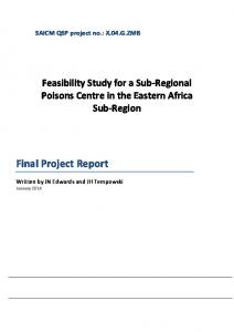
2. Modeling Protocols Most of the modeling protocols used for retrospective TexAQS-II simulations is identical to those in our AQF system. Details can be found in the interim report I “Modeling Protocols for TexAQS-II Resimulations”. Here we only highlight a few important changes made to the AQF model settings. 2.1 Domain Setup The new simulations use an extended 12-km domain “E12” for the East Texas regional domain, which covers the whole Texas and a few neighbouring states, and a 4-km standard domain “D04” covering SETX. The MM5 domains are illustrated in Figure 2.1. Corresponding CMAQ domain can be found online (http://imaqs.uh.edu/ModelSetup.html) or in the HARC-45C report Appendix A. The larger 12km domain allows our new UH-RTDAS assimilation system to ingest more observations into the MM5 runs, which should lead to better boundary conditions for the innermost domain.

Fig 2.1 MM5 domains for TexAQS-II resimulations

2.2 MM5/SMOKE/CMAQ Configurations 2.2.1 MM5 Configurations For the new simulations, we incorporated the high resolution (30 m), 26 category LULC data from UT-CSR into MM5. Our initial MM5 sensitivity test runs with year 2000 episodes showed improvements in the Ship Channel and Galveston Bay area, where the new UT-CSR LULC data differ significantly from the old USGS data. 3

_____________________________________________________________________________________________




For MM5 physical options, we generally follow the recommendations by John NielsonGammon’s group at TAMU. The options are close to the ones we adopted for project HARC-45C. • Initialization – EDAS, also ETA when EDAS is not available • Subgrid cloud convection – Grell at 36/12 km domain, no scheme at 4 km domain • Radiation scheme – RRTM • PBL scheme – UH modified MRF • LSM scheme – UH modified NOAH LSM 2.2.2 SMOKE/Emission Scenarios For the IMAQS F1 forecast system, we utilized Texas Emissions Inventory (TEI) 2 for base year 2000 to prepare the emissions inputs. The TEI inventory may overestimate emissions of ozone precursors for the 2005 episodes because several emissions control measures have been implemented since 2000. Thus, we generated an alternative emission scenario for IMAQS F2 forecast system. The emissions inventory was projected to year 2005 utilizing growth and control factors 3 . Model-ready emissions for the SAPRC99 mechanism were prepared with the Texas Emissions Inventory Processing System (TEIPS), based on SMOKE 2.1 (Sparse Matrix Operator Kernel Emissions) and EPS components to process Texas-specific emission inventories (Kim and Byun, 2003; Byun et al., 2005). The National Emissions Inventory for 1999 (NEI99) from U.S. EPA was used as a supplementary emissions without any projections to 2005 to fill in the emissions data for regions and emission species not included in the TEI. Very similar biogenic emissions inputs, estimated by the selective utilization of GloBEIS3 and BEIS3, were used in both F1 and F2 systems. One of the main reasons of using the hybrid method was to utilize the Texas-specific land use/land cover (LULC) data from TCEQ, which was more suitable for GloBEIS3 (Guenther et al., 1993; Yarwood, 2002) than the EPA’s national county-based Biogenic Emission Land-cover Database version 3. On the other hand, meteorological data such as temperature and PAR (Photosynthetically Active Radiation) were used to adjust the biogenic emissions depending on meteorological conditions forecasted by F1 and F2 meteorology, respectively. More detailed descriptions on the AQF emissions can be found from the HARC project H60 final report (Byun et al., 2006) 2.2.3 CMAQ Configurations The key CMAQ settings are listed below. In this study downscaled BCs from GEOS-CHEM were used. The BCs are quasi-dynamic – different only month by month. In a more recent study, we used the dynamic RAQMS to derive the BCs, which vary day by day. • • • • •

2 3

Chemical mechanism – CB4_aq_ae3 Boundary conditions – downscaled linkage from GEOS-CHEM Advection scheme – PPM Horizontal diffusion – multiscale Cloud scheme – RADM

ftp://ftp.tceq.state.tx.us/pub/OEPAA/TAD/Modeling/HGMCR/EI/ http://www.tceq.state.tx.us/assets/public/implementation/air/sip/sipdocs/2005-09-BPA/ado_BPA_D.pdf

4

_____________________________________________________________________________________________




3. Meteorological and Ozone Conditions for the Simulation Period An important step for air quality modeling is to understand what meteorological conditions impact lead to air quality events. The modelling period selected for the intensive TexAQS-II covers 53 days from August 14-October 5. To categorize the relation of daily weather and air quality conditions, we have performed a “weather cluster” analysis. Here we describe results of a more recent and improved categorization attempt than those provided in the earlier interim report of this project. 3.1 Weather Pattern Analysis In 2006 and 2007, IMAQS has refined the weather pattern analysis method for the SETX domain. The objective is to understand the characteristic behaviour of photochemical air pollution events under different weather patterns. The procedure is composed of a Principle Component Analysis (PCA) and a Cluster Analysis. The PCA analysis was applied to the 850 hpa wind field (U and V components) of the MM5 12-km domain at 12 UTC. Eight principal components (PCs), which explain over 80% of original variances, were retained using the in-house developed FORTRAN codes. The Cluster Analysis was then applied to the 8 PCs with the Statistical Analysis System (SAS 9.1.3) software following a two-stage (average linkage then convergent K-means) approach explained by Eder et al (1994). The combined PCA/Cluster Analysis is widely adopted for objective weather classification (2002). The procedure yields 6 clusters (named as C1, C2 to C6) excluding the weather affected by hurricanes. They are: • C1 is associated with a high pressure system that is located over the eastern states (Mississippi, Alabama etc) extending to North Atlantic Ocean. Houston is affected by southeasterly, warm and humid winds from the Gulf. • C2 occurs when Houston is located at the southern edge of a high pressure system that is centered at the north-eastern US continent. The dominant wind in Houston is easterly and wind speed is moderate. • C3 is associated with a weak synoptic pressure gradient over the domain that leads to a stagnant wind condition in Houston. In general, a weak high pressure system is over the land and a low pressure system is located in the Gulf of Mexico. Wind at the 850 hpa level is weak and variable. • C4 is associated with the cold air mass form the north-western part of the analysis domain. Houston is subject to cold and dry northerly winds. • C5 is associated with a high pressure system centered at the Gulf of Mexico. Houston is getting mild southwesterly flow. • C6 is a rare weather pattern in which Houston is placed in between a low pressure in the northwest and a high pressure system in the east, resulting in very strong southerly to southwesterly flow. Cold front is expected passing by in the following day. There were only 2 days classified into this cluster, in the summer 2005 and 2006 (May to September). 3.2 Surface Meteorological and Ozone Characteristics of Clusters The frequency of the 6 clusters in the summer 2005 and 2006 is shown in Figure 3.1. Clearly, C1 and C3 are the most dominant (popular) clusters, which account over 50% of the occurrence. 5

_____________________________________________________________________________________________




Figure 3.1 Frequency of each weather pattern cluster in summer 2005 and 2006 The dewpoint depression (T-TD) and wind speed diurnal cycle of the 6 clusters in the summer 2005 and 2006 are shown in Figure 3.2. From 3.2a, it is easy to see that the 3 “dry” clusters are C2, C3 and C4 and the 3 “wet” clusters are C1, C5 and C6. Figure 3.2b shows that the 6 weather patterns can be divided into two groups according to wind speed; C2, C3 and C4 are associate with lower wind speeds while C1 C5 and C6 with higher wind speed. The ozone diurnal cycles for the 6 clusters are presented in Figure 3.3a. Not surprisingly, the C2, C3, and C4 groups show higher ozone than the C1, C5, and C6 groups because the former groups are associated with lower winds and drier air. Strong southerly maritime air flow in the summer is associated with low ozone days in SETX. The frequency of the high ozone events for each cluster is shown in Figure 3.3b. It is clearly seen that C2, C3, and C4 are responsible for the bulk of ozone exceedances in the two summers analyzed. Note that C3 stagnant wind pattern contributes to the most ozone exceedances with the highest chance to have an exceedance. Among the CAMS sites in the whole SETX region, the site C53 (Bayland Park) has the highest ozone exceedances.

Fig 3.2a Dewpoint depression cycle of the 6 clusters Fig 3.2b Wind speed cycle of the 6 clusters Figure 3.2 Meteorological characteristics for the 6 weather patterns

6

_____________________________________________________________________________________________




Fig 3.3b Frequency of high ozone events for the 6 clusters Figure 3.3 Ozone characteristics for the 6 weather patterns

Fig 3.3a Ozone diurnal cycle of the 6 clusters

3.3 Surface Meteorological and Ozone Characteristics during 08/1/2006 – 09/30/2006 During the TexAQS II 08/1/2006 – 09/30/2006 period, all the high ozone events happened under C2, C3 and C4 (Figure 3.2). The other clusters, C1, C5 and C6 exhibit southerly to southwesterly synoptic flow on 850 hpa map, which prevented development of high ozone. Also, precipitation events occurred mostly under the C1, C5 and C6 patterns (Figure 3.2). Interestingly, non-high ozone days under the C2 and C3 patterns are associated with precipitation events. Although it must be confirmed through a detailed analysis for each day, it is suspected that the local stagnant and convergent conditions that lead to high ozone events are also conducive to the development of thunderstorms. Once thunderstorms develop, there will be little chance for ozone concentrations continue to increase. During the first half of the period (August 2006), frontal activities did not move southward far enough to reach Houston and the cool air masses stayed in the north. The C1, C2 and C5, weather patterns were prevalent with a few stagnant days (C3) in between during this period. When a high pressure system moves eastward in the north, Houston is generally subject to weak easterly flow and the weather pattern becomes C2. When a subtropical high sits in the Gulf, which occasionally extended out from the Atlantic Ocean, Houston is subject to southerly flows with high humidity. C1 and C5 are typical weather patterns in HGB when the subtropical highs are present. At the end of August, cold air gradually gained strength and moved down to HGB. Northerly flows started to appear in the 850 hpa upper weather chart. Typically, a southwesterly flow (C5) showed up on the day before the frontal passage in HGB. The days when Houston was affected by the cold air outbreak were classified as C4, as represented by the northerly winds at the 850 hpa level. On the day after the frontal passage, the flow pattern became stagnant, which is identified as C3. This synoptic cycle stays approximately 1 week and we have seen four such cycles in September 2006.

7

_____________________________________________________________________________________________




Figure 3.4 Cluster of each day during TexAQS II period (August – September, 2006) in bars. Red bars indicate high ozone events and blue diamonds indicate rainy days. The high ozone events during the period are mostly related to the frontal passages, especially during the second half of the simulation period. The high ozone events occurred under C4 when front weakened, or C3 when the warm marine air started to come back. The only ozone episode (08/04 is not a day in our simulation) not related to the frontal passage occurred during 08/16 to 08/18, which was caused by the easterly flows under C2.

8

_____________________________________________________________________________________________




4. Data Assimilation The four-dimensional data assimilation (FDDA) technique has been widely used in mesoscale modeling to limit large-scale model error growth (amplitude and phase errors). The nudging scheme, based on the Newtonian relaxation, is the most popular implementation of FDDA in MM5. It provides a continuous assimilation where artificial tendency terms are added to one or more of the prognostic equations to "nudge" the model state toward to the observed state. There are two nudging techniques - one is nudging to a grid analysis or "grid nudging", another is nudging to individual observations or "observation nudging". The National Centers for Environmental Prediction (NCEP) generates several large-scale data assimilation analysis products including EDAS every day. Therefore, almost all the MM5 nudging in USA is done with grid nudging using one of the NCEP analyses. The current MM5's nudging implementation is based on Stauffer and Seaman (1990, 1991 and 1994). While FDDA is originally intended to curb model's synoptic-scale errors, the ever-increasing observations available make it possible to apply it to a fine-scale grid (Xu et al. 2002). The application of FDDA in a fine-scale grid may have the same effect as in a synoptic-scale improving the meteorological characterization. Because air quality simulation is significantly affected by the quality of meteorological inputs that describe the local scale circulations, it may potentially improve the air quality predictions. 4.1 Development of UH Real Time Data Assimilation System (UH-RTDAS) In 2003 IMAQS developed UH-RDAS, which applies FDDA in 4-km and 12-km domains. Since the 40-km resolution EDAS analysis contains little local information, several observational datasets are ingested to the EDAS analysis to create grid analysis suited for local scale nudging. The ingestion of observation data is done in MM5's Little-R module where objective analysis is carried out. Previous studies by IMAQS have shown that fine-scale FDDA is effective in producing more realistic local circulations (Byun et al 2004). The observational datasets used in UH-RDAS include surface hourly observations from the ASOS stations and TCEQ CAMS, upper air data from NOAA radiosonde measurements and NOAA profiler networks (NPN). Dataspider programs have been written to automatically download and archive the four near real-time observation datasets. Since the data are downloaded the same day and refreshed the next day, there are still considerable missing data points in the archives. In early 2007 IMAQS discovered MADIS which has much better datasets than those used in the old UH-RDAS. Therefore it is natural for IMAQS to migrate all the observed datasets to MADIS-based. Some most important datasets in MADIS are listed below (brown datasets are used in the new data assimilation system): • •

Surface datasets (METAR, Mesonet, Buoy, COOP etc.) Upper air NOAA profiler network (NPN) ACARS (Aircraft sounding) Radiosonde data (RAWINSONDE) Satellite wind (HDW, every 3 hr) Satellite sounding (POES) Satellite radiance (SATRAD) 9

_____________________________________________________________________________________________




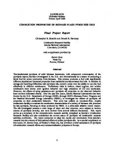
The migration to MADIS brought about several benefits. The first is that MADIS includes more data streams. Secondly, all MADIS data have been rigorously quality-checked and share a uniform data format. Thirdly, MADIS data have far fewer missing data points than our real-time archives. Figure 4.1 shows the MADIS and CAMS surface stations in E12. To take the full advantage of MADIS data a repetitive (multi-stage) nudging procedure was developed based on UH-RDAS. The new nudging system, UH-RTDAS, applies MADIS-FDDA twice in two domains. First for the 12-km domain, the objectively analyzed meteorological fields are generated in LITTLE_R by blending the MADIS and CAMS observations to the EDAS grid analysis. The output from LITTLE_R, which are organized at standard pressure levels, are then interpolated to the user-defined vertical grid in INTERPF. The results are improved IC/BC for MM5 simulation for the extended 12-km domain (E12). In addition, the surface reanalysis gridded data (for surface nudging) is generated by LITTLE_R. The 3-dimensional grid nudging is performed during the MM5 run with the data from objective analysis. Once the simulation for the 12-km resolution domain is done, the results are used to generate IC for finer 4-km domain (D04) by NESTDOWN. Similar to the E12 data assimilation, 3D grid nudging is carried out in the D04 simulation. The objective of the recursive nudging procedure is to maximize the FDDA's error correcting capabilities. The work flow of the procedure is depicted in Figure 4.2.

Figure 4.1 Surface observations in the extended E12 domain. Blue dots indicate MADIS surface stations while pink dots represent CAMS sites. Typically there are about 960 MADIS surface observations available each hour at E12 during the TexAQS-II period. Upper air (Radiosonde and NPN) and stations are not shown.

10

_____________________________________________________________________________________________




Figure 4.2 Flow chart of UH-RTDAS 4.2 Testing Various Nudging Settings UH-RTDAS is a powerful tool that could substantially improve our retrospective simulations. The next step is to find the appropriate settings for the assimilation system. These settings include: • Horizontal influence radius R – how far should an observation point influence? • Datasets – which datasets provide the most performance gain? • Domains – is bigger domain at 12-km resolution better? • Update cycle – 1-hr or 3-hourly? EDAS updated 3 hourly while observations are hourly • Simulation hours – how long should the simulation run? • Meteorological variables for nudging – using all U, V, T, and RH or selected variables? The guideline for choosing the nudging parameters is to add as much as information to the modeling system. Therefore we favour to use more datasets, more frequent update with all meteorological variables. The testing of nudging settings is divided into two phases. In Phase I, we tested influence of applying different datasets, domains, radius, and simulation hours using the day 08/31/2006. We found that using more observed datasets generally boosted performance albeit that sometimes the difference was small even with the addition of new datasets. While a bigger 12-km domain (E12) does not show visible advantage over the standard 12-km domain (D12), still we think E12 is the better choice and may benefit a different run. We used the horizontal influence radius R the same as the default setup. The 3-hourly update cycle for the 12-km domain is fine while hourly update in the 4-km domain appears to be better. For the duration of simulation hours, we find that the results for 54 hour (6 hours spin-up + 2 days) run and 30 (6 hours spin-up + 1 day) run are quite similar. The details about the Phase I simulation can be found in the interim report II - “Phase I: Testing Various Nudging Settings – Datasets, Domains, Radius, and Simulation Hours”. In Phase II, we applied the best nudging settings in Phase I (case “MNS1”) to an 8-day period (08/14/2006 to 08/21/2006) simulation. We performed MM5/CMAQ simulations for the 8 11

_____________________________________________________________________________________________




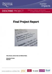
days and evaluated the results in the 4-km domain. To our surprise, the CMAQ results are not as good as expected. Although the MNS1 wind field statistics such as correlation and IOA are better than AQF in all 8 days, the ozone statistics showed that AQF has better ozone simulations on August 14-15 and August 19. Further examination revealed that nudging caused unrealistic thunderstorms that are not present in the AQF case in these three days. The thunderstorms are easily identifiable as “star-bursting” patterns in spatial wind vector plots. The presence of the bogus thunderstorms can seriously distort the regional flow and degrade the performance of CMAQ runs. The reason that the distortion is not reflected in the statistics (e.g., correlation or IOA) is that the thunderstorms typically occur in areas with few or no observations. Since the statistics are calculated by comparing model/observation pairs at observation sites, the statistics alone do not reflect the flows in other areas. Because what nudging does is to relax model state at grid cells around observation sites and “nudge” it toward observation, the statistics of nudged parameters almost always improve. On the other hand, the chemistry fields are sensitive to the overall flow field and their statistics are more reliable indicators. The discovery, along with suggestions from outside IMAQS, led us to nudge only wind components (U, V) in the 4-km domain. Besides the thunderstorm issue, we also found that the lateral boundary winds in MNS1 sometimes are worse than AQF’s. This led us to add the 36-km domain MM5 run on top of the 12-km and 4-km domain runs in MNS1. Additionally we discovered an issue in the EPA’s standard MCIP release, such that the minimum boundary layer height is being set to the lowest model layer height. For HGB, the night-time boundary layer height is usually much higher than the lowest model layer height. For this we modified MCIP to set the minimum boundary layer height to a fixed value (mostly 50 m, except for urban, which is set at 300 m). At the end of Phase II, we identified the case “TMNS11n2” as the best. For detailed configurations of TMNS11n2, please see “Introduction” section of this report. For more details about the Phase II simulation, please see our interim report III - “Phase II: Thunderstorm Issues, Nudging with Selected Weather Parameters”. 4.3 An Example Demonstrating the Advantage of Improved Data Assimilation Here, to demonstrate that the assimilated meteorological data improved air quality simulation, we provide an example comparing two sets of CMAQ simulations, AQFn (“n” denotes boundary layer height corrected) and TMNS11n2 (shown as TMNS11n in the plots below). Both sets of CMAQ runs use the same IMAQS-F2 emission (section 2.2.2). The episode simulated is 08/17/2006, classified as weather pattern C2 in IMAQS’s weather pattern analysis (section 3.3). On August 17, the clouds are scattered (closer to clear sky than broken clouds) and the day is dry. In early morning, winds were converging from north, west and east near the Houston Ship Channel (SC) area then moved south. Pollutants were also carried south-SSE. Starting from 9 CST, winds were light near the Ship Channel and ozone started to rise around and at South of the Ship Channel (Pasadena, Clear Lake, and Seabrook). At 11 CST, ozone reached 92 ppb in Baytown. Gradually, winds turned to easterly bringing ozone plume to the west. Ozone reached 147 ppb at 13 CST at Deer Park. In the afternoon, winds were generally north-easterly to easterly in the whole region, continuously moving the plume west and a bit south. By 17 CST, high ozone located near the intersection of High Way 288 and Beltway 8. Figure 4.3 shows the spatial wind plots at 15 CST on August 17, 2006. Most notable is that the winds in TMNS11n2 were weaker than those in AQFn and matched better with observations. The wind patterns at southwest Houston, Fort Bend County, and Brazoria County are different between the two cases. Winds in AQFn are consistently northeasterly while winds in TMNS11n2 show two separate regimes. In TMNS11n2, there is a convergence zone around the south/southwest Beltway 8 area, as shown in the observations. The location and strength of the convergence zone are quite important in determining formation of high ozone in the region. Clearly, 12

_____________________________________________________________________________________________




the data assimilation successfully nudged winds in TMNS11n2 representing the observed wind patterns that led to the high ozone event on this day.

Figure 4.3 Spatial wind plots for AQFn and TMNS11n2 at 2006.08.17:15 CST. It shows that TMNS11n2 captures ozone spatial pattern better. Red arrows are observations. Figure 4.4 shows the spatial ozone plot at 15 CST. Observed ozone reached its peak of 158 ppb at C558 (Houston Tom Bass). The TMNS11n2 case reproduced observed ozone distribution better than the AQFn case. The high ozone area in the AQFn case was located far too southwest and the intensity was less than observed. This is in agreement with its wind pattern – the northeast wind in AQFn was too strong in the day and pushed the high ozone area further to Fort Bend and Brazoria. On the other hand, in TMNS11n2, the convergence zone located at south/southeast Beltway 8 was able to produce a more realistic spatial ozone picture albeit the northwesterly in TMNS11n2 was still a bit too strong and pushed the high ozone area to the west a little too far.

Figure 4.4 Spatial ozone plots for AQFn and TMNS11n at 2006.08.17:15 CST. It shows that TMNS11n captures ozone spatial pattern better. Circles are observations.

13

_____________________________________________________________________________________________




5. Modeling Results for 08/14/2006 - 10/05/2006: Meteorology For the evaluation of simulated meteorology over the selected TexAQS-II period (08/14/2006 - 10/05/2006), we choose two case of model simulations: AQF (which is the original forecast run) and TMNS11n2. AQFn case (meteorology and chemistry) was run only for the first 8 days, therefore not suitable for the comparison here. As a common practice, we focus our analyses in the 4-km SETX domain which has the most available observations. • • • • •

The observation data and images we collected for the evaluation include: Surface observations – CAMS, MADIS sfc (including ASOS, buoy, coop etc); for precipitation, we found hourly data from CAMS and ASOS sites. Upper air observations – RAOBS, NPN/MAP, ACARS Satellite images – GOES-12 imagery, Visible Channel 30 (per TCEQ), showing water vapour. Radar images – hourly Doppler imagery, showing precipitation

Due to the long simulation period, we present model results in two set of hourly time series plots. The first set covers 08/14/2006 - 09/13/2006 and the second set cover 09/14/2006 – 10/05/2006. For time series plots, the regional averages are displayed. The regional average is calculated using all available CAMS sites, but it is not the true spatial average. When needed, time series for the following five selected CAMS sites are presented: • C8 – Aldine; subject to high ozone when S/SE flows carry SC plumes to the site • C552 – Baytown; subject to high ozone during stagnant conditions • C34 – Galveston; an effective proxy of background ozone • C81 – TCEQ regional office; close to UH, SC plumes were brought westward to the site during easterly flow conditions • C53 – Bayland park; the site with the most ozone exceedance The regional average plots for temperature, relative humidity, U-wind, V-wind and wind speed are shown in Figures 5.1 through 5.5.

(a)

14

_____________________________________________________________________________________________




(b) Figure 5.1 Time series plot of regional average temperature; (a) - 08/14/2006 - 09/13/2006, (b) 09/14/2006 - 10/05/2006

(a)

(b) Figure 5.2 Time series plot of regional relative humidity; (a) - 08/14/2006 - 09/13/2006, (b) 09/14/2006 - 10/05/2006

(a) 15

_____________________________________________________________________________________________




(b) Figure 5.3 Time series plot of regional U-wind; (a) - 08/14/2006 - 09/13/2006, (b) - 09/14/2006 10/05/2006

(a)

(b) Figure 5.4 Time series plot of regional V-wind; (a) - 08/14/2006 - 09/13/2006, (b) - 09/14/2006 10/05/2006

(a) 16

_____________________________________________________________________________________________




(b) Figure 5.5 Time series plot of regional wind speed; (a) - 08/14/2006 - 09/13/2006, (b) 09/14/2006 - 10/05/2006 Highlights from the surface temperature time series (Figure 5.1) ¾ Surface (1.5 m) temperature are very well simulated overall ¾ For a few days, e.g., 08/23, 08/26, 09/09, model overpredicted the low ozone values in the daytime due to the MM5’s failure simulating the precipitation events in HGB. This is a wellknown issue for meteorological models, which often show difficulties in simulating precipitation events and associated clouds at specific locations. ¾ Model tends to slightly overpredict night-time temperature lows, which is likely to be associated to the night-time wind overprediction and too thick layer used to represent surface variations. ¾ TMNS11n2 outperformed AQF in some days while AQF did better in a few other days. However, the difference in performance is not quite significant from the regional average plot. It should be noted that there is no surface RH and temperature nudging in the 4-km domain analyzed here. Highlights from the surface relative humidity time series (Figure 5.2) ¾ Relative humidity are well simulated. ¾ Observed RH values are slightly higher at night, which is not a surprise. This is because model’s lowest layer height is 34 m, higher than the 1.5 m observation height. Surface temperature is typically lower than higher level due to the night-time surface radiation cooling, especially during the nights with clear sky. ¾ In a few nights, such as 08/29 to 08/30, model overpredicted the humidity probably due to the cold front moving across the region. The model often shows westerly flows during the night while observation has mostly northerly flows. This explains the drier air in the observation since air mass dominated the region is the cooler air from the north. ¾ In some other nights, notably the 09/19 to 09/20 and 09/25 to 09/27 nights, model underpredicted the RH, which is probably due to the model temperature overprediction. These are the days when cold fronts swept down the region, accompanied by dry and cold air mass. Highlights from surface wind time series (Figures 5.3 - 5.5) ¾ Model surface wind pattern compares well with observation, especially for the V-wind component. 17

_____________________________________________________________________________________________




¾ AQF has higher wind speed than observation with a higher day-time peak and a higher night-time low in most of the days (Figure 5.5). It is also interesting to see the delayed daytime peak hour in the model. ¾ Although TMNS11n2 slightly overpredicted wind speed, it shows a dramatic improvement over AQF. The night-time low follows observation much better. ¾ Model showed much higher skill in simulating V-wind than U-wind. The simulated U-wind magnitude tended to be slightly higher than observation while the situation is much milder in V-wind magnitude. ¾ There is a much larger bias in AQF’s negative U-wind component (i.e., stronger easterly) in many days. The strong easterly is likely a result of improper synoptic winds provided by the NCEP analysis data used. The bias was reduced significantly in TMNS11n2 due to the data assimilation. ¾ For V-wind component, the bias is less than the U-component. The bias is mostly related with the nocturnal wind speed. Model generally has higher southerly under weather pattern C1 and C5, as well as stronger northerly as fronts pass the region (weather pattern C4). ¾ The stronger model winds at night suggest that the frictional effects are not well represented in the model. Either the model layer was too thick or model’s roughness length for the HGB may not reflect the expansive urban surface structures properly.

18

_____________________________________________________________________________________________




6. Modeling Results for 08/14/2006 - 10/05/2006: Chemistry The regional average plots for model simulated CO, NO, NO2 and ozone are shown in Figures 6.1 through 6.4. Highlights from CO time series (Figure 6.1) Since there are fewer CAMS taking CO measurements and there are known issues in CO measurements such as the “jumping” and “persisting” due to instrumental response or other problems, one need to use more caution when interpreting the CO analyses. ¾ Overall, model simulated CO reasonably well although model had much more pronounced daytime peaks than observation. The TMNS11n2 performed better than AQF with less high biases of morning peaks in most of the days. ¾ As expected from the analysis of meteorological time series, we see problems in simulating CO on 08/23 and 08/26, and 09/05, 09/09, and 09/11 stemming from the poor simulation of precipitation events. It seems that large morning bias for 8/27 – 8/28 are due to misrepresentation of morning planetary boundary layer (PBL) growth and overnight cloudiness, and 9/14 may be due to wind pattern errors. ¾ Still, there are other mismatches, which are difficult to identify the causes, such as the nights of 09/01-09/02 and 09/12-09/13.

(a)

(b) Figure 6.1 Time series plot of regional average CO; (a) 08/14- 09/13/2006, (b) 09/14- 10/05/2006

Highlights from NO and NO2 time series (Figures 6.2 and 6.3) 19

_____________________________________________________________________________________________




¾ There is a general underprediction of NO during the night and early morning hours. It corresponds with the model NO2 overprediction. The biases are expected because of the thicknesses of model layers are not fine enough to resolve the rapid titration reaction of O3 with emitted NO forming NO2 at night. ¾ Model NO2 prediction shows much larger biases than NO prediction during most of the diurnal cycle.

(a)

(b) Figure 6.2 Time series plot of regional average NO; (a) 08/14- 09/13/2006, (b) 09/14- 10/05/2006

20

_____________________________________________________________________________________________




(a)

(b) Figure 6.3 Time series plot of regional average NO2; (a) 08/14- 09/13/2006, (b) 09/14- 10/05/2006

(a)

(b) Figure 6.4 Time series plot of regional average O3; (a) 08/14- 09/13/2006, (b) 09/14- 10/05/2006

21

_____________________________________________________________________________________________




Highlights from ozone time series (Figure 6.4) ¾ Model generally captured the daily ozone cycle well, although there were some night-time overprediction which we observed from our past simulations. ¾ One problem with the ozone simulation during the period occurred on 08/23. Both model runs significantly overpredicted the daytime peak. There are likely two causes for the overprediction. The first is that model had fewer clouds (and accompanying precipitation) than observation – the satellite images showed that there were large stretch of clouds coming from the east and southeast. This effect lingered for the following two days (8/24 – 8/25) showing serious high biases in the predicted ozone. ¾ Another problem shows during the southerly wind days (i.e., positive V-wind component days, such as 8/26 - 8/28), the model overpredicted ozone by around 10 to15 ppb. Figure 6.6 shows the ozone time series plot at Galveston – observed ozone was quite low during the period while model ozone is rather high which indicated that Galveston was dominated by marine air mass. This suggests that the model boundary ozone concentrations, which were provided through downscaling of year 2002 monthly average GEOS-Chem model output using 36-km and 12-km nested CMAQ simulations, are set too high to represent the air from the Gulf of Mexico. Overprediction of ozone during 9/9 – 9/12 are also attributed to both the missing precipitation and some weaker southerly flows in the MM5 simulations compared to the observations. ¾ There is a distinct large overprediction of ozone on 09/15 by the CMAQ simulation with the assimilated meteorology. Inspection of regional flow patterns and 12-km domain simulation shows that the bias on 09/15 is caused by the transport of very high simulated ozone plume originated from the New Orleans area moved over the Gulf. CAMS and surface measurements do not support such high ozone in the coastal area. ¾ About 10-15 ppb ozone biases are shown for 09/16 – 09/17 and 09/21 – 09/23 periods, both under the persistent southerly flow conditions, are again due to the high background ozone in the Gulf. ¾ Significant overprediction of regional average ozone concentrations on 9/30 – 10/01 is probably caused by the much less cloud cover simulated by MM5. Inspection of satellite picture (not shown) indicates that extensive low-level clouds covered the HGB area, where the advancing cold and dry continental air collided with humid Gulf air mass. ¾ Though both AQF and TMNS11n2 overpredicted after cold front passed, TMNS11n2 displayed less overprediction than AQF. This is possibly due to the improved wind simulation in TMNS11n2 that carried in less enhanced ozone from the Gulf.

22

_____________________________________________________________________________________________




(a)

(b) Figure 6.5 Ozone time series plot at Baytown C552: (a) 08/14/2006 - 09/13/2006, (b) 09/1410/05/2006

(a)

(b) Figure 6.6 Ozone time series plot at Galveston C34: (a) 08/14/2006 - 09/13/2006, (b) , (b) 09/1410/05/2006

23

_____________________________________________________________________________________________




7. Concluding Remarks The research conducted in this project aimed to develop a series of high quality MM5 and CMAQ simulations commensurate with the CAMS measurements during the TexAQS-II period. To achieve better meteorological simulations we primarily relied on enhanced data assimilation with newly available datasets such as the high resolution land use/land cover (LULC) dataset, and the addition of various data streams from MADIS. Additionally, we implemented a few changes in the MCIP code to obtain a better meteorological representation in the lowest model layer. Although our new MM5 simulations performed reasonably well in predicting day-to-day meteorology, occasionally they were negatively impacted by the inaccurate synoptic conditions coming from EDAS. For example, during 08/23 to 08/26, there were strong northeasterly flows in the model due to the overly intensified low pressure systems in the Gulf of Mexico which lead to the ozone overprediction in CMAQ simulations. Our performance evaluation showed the new meteorological data and the new FDDA system (UH-RTDAS) generally improved the MM5 simulations. Sometimes the improved FDDA dramatically enhanced the local flow field which led to much more realistic chemistry simulations. However, it appeared that the inaccurate synoptic conditions exerted a larger impact than the data assimilation system; hence the success of FDDA relied on a good set of synoptic conditions. Therefore, we plan to switch to a newer analysis product such as the North American Regional Reanalysis (NARR) in our next round of simulations. Our modelled air temperatures agreed well with observations except for a few days when model had difficulties in simulating precipitation events and associated clouds at specific locations. Time series plots for the wind components and speed showed that the meteorological model simulated synoptic changes well, especially the V-wind component. Sometimes there were serious overprediction of easterlies and slight overprediction of northerlies in our original AQF case, and the overprediction moderated in the new TMNS11n2 case. The new case also brought down the night-time wind in the AQF case. Overall the assimilated meteorological inputs improved our air quality simulations. The CMAQ re-simulations with the TMNS11n2 meteorology inputs predict locations and magnitudes of peak ozone better than those in the original AQF runs. The spatial and scatter plots all show that TMNS11n2 meteorology outperforms AQF. CMAQ simulations with the AQF emissions and TMNS11n2 meteorological inputs compare well with observations although the regional averages show some overprediction of ozone during the morning hours. Similar to the synoptic meteorology conditions, the problematic chemistry boundary conditions can bring notable bias to the inner domain. There were some instances when incorrect simulation of clouds and precipitation fields resulted in serious discrepancies in the simulated ozone and other instances when significant ozone biases were caused by the incorrect transport of ozone and its precursors were transported from boundaries under southerly or south-easterly flow conditions, especially after the passage of cold front over the HGB region.

24

_____________________________________________________________________________________________




8. References Byun, D. W., S. B. Kim, N. K. Moon, F. Ngan, Y. Li and T. Ng, 2004: Real-Time Trajectory Analysis Operation and Tool Development. HARC Project No: H19.2003. Byun, D.W., S. Kim, F.Y. Cheng, B. Czader, I.-B. Oh, M. Jang, C.-K. Song, H.-C. Kim, P. Percell, F. Ngan, V. Coarfa, and D. Cohan, 2006: HARC Project H60 Final Report. Regional Air Pollution Transport Modeling: Application of CMAQ/HDDM Simulations on Ozone Concentrations over Dallas and Houston Areas, IMAQS, University of Houston, Houston, Texas. (http://files.harc.edu/Projects/AirQuality/Projects/H060/H60UHFinalReport.pdf) Eder, B. K., J. M. Davis and P. Bloomfield, 1994: An Automated Classification Scheme Designed to Better Elucidate the Dependence of Ozone on Meteorology. J. Appl. Meteor., 33, 1182-1199. Jolliffe, I., 2002: Principal component analysis. Springer. Second edition. Guenther, A. B., P. R. Zimmerman, P. C. Harley, R. K. Monson, and R. Fall, 1993: Isoprene and monoterpene emission rate variability: model evaluations and sensitivity analyses. J. Geophys. Res., 98D, 12609-12617. Stauffer, D.R., and N.L. Seaman, 1990: Use of Four-Dimensional Data Assimilation in a Limited-Area Mesoscale Model. Part I: Experiments with Synoptic-Scale Data. Mon. Wea. Rev., 118, 1250–1277. Stauffer, D.R., N.L. Seaman, and F.S. Binkowski, 1991: Use of Four-Dimensional Data Assimilation in a Limited-Area Mesoscale Model Part II: Effects of Data Assimilation within the Planetary Boundary Layer. Mon. Wea. Rev., 119, 734–754. Stauffer, D.R., and N.L. Seaman, 1994: Multiscale Four-Dimensional Data Assimilation. J. Appl. Meteor., 33, 416–434. Xu, M., Y. Liu, C. Davis and T. Warner, 2002: Sensitivity study on nudging parameters for a mesoscale FDDA system. 15th Conference on Numerical Weather Prediction, 12-16 August, 2002, San Antonio, Taxes. 4B4. Yarwood, G., Wilson, G., and S. Shepard, 2002: User’s Guide to the Global Biosphere Emissions and Interactions System (GloBEIS) Version 3; ENVIRON International Corporation.

25

_____________________________________________________________________________________________



2007 TexAQS-II Modeling Project: Final Report - TCEQ

2007 TexAQS-II Modeling Project: Final Report - TCEQ

Suggest Documents

2007 TexAQS-II Modeling Project: Final Report - TCEQ

Offshore Oil and Gas Platform Report FINAL REPORT - TCEQ

FINAL REPORT January 2007

project final report - MIROR Project

ucmexus final project report ucmexus final project report - University of ...

Final Report O3SAF-VS, 2007

Final Project Report

Masters Project Final Report

Final GIS Project Report

PROJECT FINAL REPORT

Final Report - FAROS Project

Final project report

Final Project Report

Final Project Report

project final report - TECA

Final Project Report

Project Final Report

NDOT 2007-12 Final Report

Final Project Report

project final report - CORDIS

Final Project Report

Final Project Report

project final report - bambi

FINAL PROJECT REPORT