Xerox Palo Alto Research Center, 3333 Coyote Hill Road .... and 4 then give âcoroutinesâ for the inductive step; each of these lemmas calls the other on a ..... later. Assume the triangle is ace and its inbound side is horizontal base ae. If cae. 9 ...
International Journal of Computational Geometry & Applications, Vol. 2, No. 3 (1992) 241–255 c World Scientific Publishing Company °
POLYNOMIAL-SIZE NONOBTUSE TRIANGULATION OF POLYGONS
MARSHALL BERN Xerox Palo Alto Research Center, 3333 Coyote Hill Road Palo Alto, California 94304, U.S.A.
and DAVID EPPSTEIN Department of Information and Computer Science, University of California Irvine, California 92717, U.S.A.
Received 11 May 1991 Revised 6 June 1992 ABSTRACT We describe methods for triangulating polygonal regions of the plane so that no triangle has a large angle. Our main result is that a polygon with n sides can be triangulated with O(n2 ) nonobtuse triangles. We also show that any triangulation (without Steiner points) of a simple polygon has a refinement with O(n4 ) nonobtuse triangles. Finally we show that a triangulation whose dual is a path has a refinement with only O(n2 ) nonobtuse triangles. Keywords: Computational geometry, mesh generation, triangulation, angle condition.
1. Introduction One of the classical motivations for problems in computational geometry has been automatic mesh generation for finite element methods. In particular, mesh generation has motivated a number of triangulation algorithms, such as finding a triangulation that minimizes the maximum angle.1 A triangulation algorithm takes a geometric input, typically a point set or polygonal region, and produces an output that is a triangulation of the input. For a point set, this usually means partitioning the region bounded by its convex hull into triangles, such that the vertices of the triangles are exactly the input vertices. Triangulating a polygonal region usually means partitioning the region into triangles such that the vertices of the triangles are exactly the vertices of the region’s boundary. In both cases, the output must be a simplicial complex, that is, triangles intersect only at shared vertices or edges. Mesh generation applications, however, invariably place further requirements on the triangulation, stemming from numerical analysis. Very flat and very sharp angles are undesirable.2,3 To satisfy angle bounds, it may be necessary to augment 1
the input by adding new vertices, called Steiner points. Because the complexity of the finite element computation depends on the size of the mesh, the number of Steiner points should be kept small. Until recently, computational geometers neglected the more realistic Steiner versions of triangulation problems, and concentrated on problems that do not allow extra vertices. An upper bound of 90◦ has special importance in mesh generation. A triangulation of a point set with maximum angle 90◦ is necessarily the Delaunay triangulation. In finite element methods for solving certain partial differential equations, a nonobtuse mesh leads to a matrix with nice numerical propertices, such as all off-diagonal elements being nonpositive.4 For a more geometric motivation, notice that each (closed) triangle in a triangulation contains the center of its circumscribing circle exactly when all angles measure at most 90◦ . The “perpendicular planar dual” of such a triangulation can be formed by simply joining perpendicular bisectors of edges. Practitioners often use a mesh and its dual—sometimes with bent edges in the dual—to discretize vector fields.4 In general, a straight-line embedding of the planar dual of a triangular mesh can be formed by placing dual vertices at the meeting point of angle bisectors5 ; however, a perpendicular planar dual is more accurate and simplifies the calculation of flow or forces across element boundaries. 1.1. Summary of Results In this paper we consider the problem of triangulating a polygonal region so that all angles measure at most 90◦ . We give the first algorithm that produces such a nonobtuse triangulation with size (number of triangles) bounded by a polynomial in n, the number of sides of the input polygon. The only previous provably-correct algorithms, due to Baker et al.,4 have no size guarantees. Indeed, the size of the triangulations produced by the algorithms of Baker et al. depend on the geometry of the input, and hence can be arbitrarily large, even when n is fixed. Our main result is that an arbitrary polygon can be triangulated with O(n2 ) nonobtuse triangles. The polygon need not be simple; it may contain polygonal holes. We also consider the problem of refining a given triangulation of a polygon (without Steiner points) into a nonobtuse triangulation. We achieve O(n4 ) triangles for arbitrary simple polygons, and O(n2 ) for the special case of a polygon with a “path triangulation”, that is, a triangulation whose dual is a path. All our algorithms can be made to run in time O(n log n + k), where k is the size of the output. Our angle bound is the best possible for polynomial-size triangulations. Our work with John R. Gilbert6 shows that any smaller fixed bound on the largest angle would require the number of triangles to depend not only on the size of the input, but also on its aspect ratio. Consider for example an input that is an extremely long, thin rectangle R. A triangle with a maximum angle of, say, 89◦ must have longest side no longer than a constant multiple of R’s smaller dimension, and hence a large number of these triangles would be needed to cover R.
2
1.2. Related Work The original computational geometry result motivated by mesh generation is that the Delaunay triangulation of a point set maximizes the minimum angle.7,8,9 (It is a curiously similar fact that, for points in convex position, the farthest-point Delaunay triangulation minimizes the minimum angle.10 ) For polygons the minimum angle is maximized by the constrained Delaunay triangulation.11,12 It is also known how to compute the triangulations that minimize the maximum angle,1 maximize the minimum triangle height,13 and minimize the maximum triangle “eccentricity”13 for both point sets and polygons. Theoretical work on Steiner triangulation problems is less common. In an earlier paper,6 we developed algorithms based on quadtrees for a number of Steiner triangulation problems. In a certain strong sense, we solved the problems of Steinertriangulating point sets and polygonal regions with no small angles (when the minimum angle bound is sufficiently small, for example no more than 18.4◦ ). For each input our algorithms produce an output that has size within a constant factor of the optimal size. The number of triangles required necessarily depends not only on the size of the input, but also on its aspect ratio. We also showed how to triangulate point sets with no large angles. If the angle bound is less than 90◦ , the solution is essentially identical to that for no small angles; but if the only requirement is that there be no obtuse angles, the point set can be triangulated with only linearly many Steiner points. Gerver14 showed how to compute a nonpolynomial-size triangulation of a polygon with no angles larger than 72◦ , assuming all interior angles of the input measure at least 36◦ . As mentioned above, Baker et al.4 gave a nonpolynomial algorithm for nonobtuse triangulation, thereby showing that every polygon has such a triangulation. They gave a simple algorithm for nonobtuse triangulation of a polygon whose vertices have integer coordinates. This algorithm imposes a unit grid on the polygon, so it typically uses an exponential (in the size of the encoding of the input) number of triangles. They went on to give a somewhat more complicated algorithm for the general problem. This second algorithm also avoids angles smaller than 14◦ , and is thus inherently nonpolynomial as well. Our earlier result that point sets can be triangulated with O(n) nonobtuse triangles led us to suspect that polygons too could be triangulated with a polynomial number of nonobtuse triangles. Subsequent to the work reported here, Eppstein devised an algorithm that triangulates a convex polygon with O(n1.85 ) nonobtuse triangles (included in Ref. 18). 2. Obtuse with subdivided legs In this section, we develop the main subroutine of our nonobtuse triangulation algorithm. In the next section, we shall present the full algorithm. Throughout this paper, we use hypotenuse to mean the longest side of a triangle and legs to mean the other two sides. A subdivision point is a vertex of a polygon at which the angle measures 180◦ . A nonobtuse (nonacute) angle is one measuring at most
3
(respectively, at least) 90◦ . The measure of angle 6 abc is denoted |6 abc|. Suppose we are given a triangle ace with hypotenuse ae as its horizontal base, with |6 ace| ≥ 90◦ , and with subdivided legs. In this section we show how to triangulate this input into nonobtuse triangles, without adding any new subdivision points to the legs. Our overall stategy is to replace the legs by ones sloped slightly closer to the horizontal, while keeping the base fixed. The region between the old legs and the new legs is triangulated in such a way as to reduce the total number of subdivision points by one. The remaining subdivision points propagate towards the polygon boundary.
Figure 1. Base cases.
We have two different reduction methods, called apex merger and side merger . Roughly speaking, an apex merger combines the first subdivision point on one leg with apex c; a side merger combines two closely-spaced subdivision points. The reduction methods given here have been simplified somewhat from the reduction methods given in the conference version of this paper.15 Our first two lemmas and Figure 1 give the basis of an induction. Lemmas 3 and 4 then give “coroutines” for the inductive step; each of these lemmas calls the other on a triangle with at most n − 1 subdivision points. Lemma 1. If ace is a right triangle with one subdivision point on a leg, ace can be triangulated into three right triangles, with one subdivision point on base ae. Proof. Simply add the edge from the subdivision point to the opposite vertex of ace; then drop the altitude from the subdivision point perpendicular to base ae. 2 Lemma 2. If triangle ace is obtuse with no subdivision points, then it can be triangulated into two nonobtuse triangles, adding one subdivision to base ae. Proof. Simply drop the altitude from c to ae. 2 Lemma 3. Assume nonacute triangle ace has n ≥ 1 subdivision points, all on one leg. Using O(n) nonobtuse triangles, either we can reduce the untriangulated portion of ace to a nonacute triangle ac0 e with n − 1 subdivision points, or we can completely triangulate ace adding at most n + 1 subdivision points to base ae. Proof. Without loss of generality, assume ac is the subdivided leg, and let b be the subdivision point closest to c. If |6 ace| = 90◦ , we simply add edge be and reduce to the case of an obtuse triangle with n − 1 subdivision points. So assume |6 ace| > 90◦ , and consider extending a perpendicular to ac at b and a perpendicular to ce at c. Assume these meet at point c0 inside the (closed) triangle ace. Now imagine adding edges that project the subdivision points along ac onto 4
c b
c b c’ c’
a
e
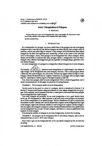
Figure 2. (a) Apex merger.
a
e
(b) Side merger.
ac0 , alternately projecting perpendicularly away from ac and perpendicularly onto ac0 . The first subdivision point b projects away (to point c’), the next one down from b projects onto, and so forth. See Figure 2(a). Now if 6 bac0 is sufficiently small (relative to the spacing of subdivision points), then none of these projection edges cross each other, and triangle abc0 will be divided into some number of quadrilaterals and one right triangle. Each quadrilateral has the nice property that it can be divided into two right triangles with a diagonal. This move, in which we reduce the number of subdivision points by combining the apex and an adjacent subdivision point using the meeting point of perpendiculars, is called an apex merger . So assume that the perpendiculars to ac at b and to ce at c do not meet at a point c0 with sufficiently small 6 bac0 . Instead define c0 to be the last point (i.e., furthest from b) in triangle ace along the perpendicular to ac at b, such that the projection edges from ac do not cross. (Two line segments cross if they intersect at a point that is interior to each segment.) Notice that |6 c0 ce| > 90◦ since the apex merger did not succeed. One possibility is that c0 lies on base ae. (This case occurs whenever n ≤ 2 and the apex merger fails.) We add the projection edges from ac to ac0 , along with c0 c, and drop an altitude from c to c0 e. Quadrilaterals are triangulated as before into two right triangles. Now there is no untriangulated portion of ace, and the number of Steiner points on base ae is at most n + 1. Look at Figure 2(b) and imagine c0 lying on base ae. The other possibility is that c0 lies interior to ace. Now by our choice of c0 some adjacent pair of projection edges meet along ac0 , as shown in Figure 2(b). Along with the projection edges and quadrilateral diagonals, we add cc0 , c0 e, and an altitude from c to c0 e. Triangle ac0 e has at most n−1 subdivision points, although one of them has now moved to the right leg (necessitating Lemma 4 below). This reduction step is called a side merger . 2 Notice that the algorithm given in the proof of Lemma 3 either reduces the number of subdivision points by one without adding anything to base ae, or it completely triangulates ace. The same will be true of our method for the case of subdivisions on both legs. Therefore, we assert that the algorithm given by Lemmas 1–4 adds at most n + 1 points to the base, and at most n if ace is right. Because each merger uses O(n) triangles and removes one subdivision point, the total number of triangles will be O(n(n − n0 + 2)), where n0 is the number of subdivisions added to the base. We use these bounds recursively in the proof of the next lemma.
5
c
c b
d
b
c’
a
d c’
e
a
e
Figure 3. In both apex (a) and side (b) mergers, c0 de is triangulated recursively.
Lemma 4. Assume triangle ace has n ≥ 2 subdivision points, with at least one on each leg. Using O(n(n − n0 + 2)) triangles, either we can reduce the untriangulated portion of ace to a nonacute triangle ac0 e with n0 ≤ n − 1 subdivision points, or we can completely triangulate ace adding n0 ≤ n + 1 subdivisions to the base. Proof. Let b and d be the closest subdivision points to c on ac and ce, respectively. Let nr represent the number of subdivision points on the right leg ce. We first try the apex merger of c with b. Assume that the perpendiculars to ac at b and to ce at c meet at point c0 in ace, such that 6 cac0 is small enough that no projection edges cross, as shown in Figure 3(a). In this case, we add edges c0 d and c0 e. Triangle c0 de has nr − 1 subdivisions, all one leg, so we can triangulate it recursively, outputting at most nr subdivisions on base c0 e. Thus we have reduced the problem to triangulating ac0 e, an obtuse triangle with one fewer subdivisions. So assume the apex merger of c and b is not possible, and let c0 be the last point in triangle ace along the perpendicular to ac at b such that no pair of adjacent projection edges from ab onto ac0 cross. Since the apex merger failed, 6 c0 cd is obtuse. Now if c0 lies on base ae, then we add edges bc0 , c0 c, and c0 d; drop an altitude from c to c0 d; and triangulate the quadrilaterals along ab. These steps add n − nr subdivision points to base ae and reduce the problem to triangulating c0 de, an obtuse triangle with nr subdivisions (on two legs). Triangle c0 de is triangulated recursively, adding at most nr + 1 subdivision points to ae, for a total of at most n + 1. Because each merger removes a subdivision point at the cost of O(n) new triangles, the total number of triangles used will be O(n(n − n0 + 2)), where n0 is the number of subdivision points added to ae. The remaining possibility is that c0 lies interior to ace. In this case, we can perform a side merger. We add edges c0 c, c0 d, c0 e, and an altitude from c onto c0 d, as shown in Figure 3(b). We then triangulate c0 de recursively. After this step, triangle ac0 e has at most nr + 1 subdivisions on leg c0 e and n − nr − 2 on leg ab0 (one fewer due to the merger and another fewer because c0 is the apex and not counted as a subdivision point), so the total number of subdivision points is at most n − 1. As throughout, the number of triangles used in this step is O(n) per subdivision point removed. 2 Theorem 1. An obtuse or right triangle with n subdivisions on its legs can be triangulated with O(n2 ) nonobtuse triangles, without adding any new subdivisions to the legs. 2
6
3. Arbitrary Polygons We now show how the method of the previous section can be applied to an arbitrary polygon, possibly with holes. Our overall strategy is to partition the polygon into some simple shapes, by cutting it with horizontal and vertical lines. Each such shape can be either triangulated directly or divided into obtuse triangles with subdivided legs, that can then be further triangulated using the methods developed to prove Theorem 1. Draw a vertical line segment through each vertex of the polygon, extending to the boundaries of the polygon. These lines divide the polygons into slabs, which we define as quadrilaterals with two vertical sides, possibly with subdivision points on the vertical sides. In degenerate cases, two vertices may lie on the same vertical line; this causes no problems. Each vertex of a slab will be either an original input vertex, or a point where a vertical line touches the polygon boundary. Draw a horizontal line segment through each slab vertex, and extend the line segment to the last possible vertical segment. In other words, each endpoint of a horizontal segment should lie either on a vertical segment, or on the vertex inducing the horizontal, and each horizontal segment should be as long as possible with this property. A polygon so divided is shown in Figure 4(a). Lemma 5. The above steps partition the polygon into regions of four types: (1) rectangles with unsubdivided sides; (2) right triangles with hypotenuse on the boundary of the polygon and vertical leg possibly subdivided; (3) obtuse triangles with two sides on the boundary of the polygon, and one leg vertical and possibly subdivided; (4) slabs with two sides on the boundary of the polygon, and two possibly-subdivided vertical sides, that cannot be simultaneously crossed by a horizontal line. Proof. Any other shape must have a vertex from which a line segment can be extended vertically or horizontally. The construction only creates verticals and horizontals, so any other line segments must be on the polygon boundary. 2 Theorem 2. Any n-vertex polygon (with holes) can be triangulated with O(n2 ) nonobtuse triangles. Proof. We apply the procedure above to subdivide the polygon into the shapes listed in Lemma 5. Triangulating the rectangles is trivial. The right and obtuse triangles can be triangulated by the method of the previous section. The slabs can be divided by a diagonal into two obtuse triangles, that can then be triangulated by the method of the previous section. See Figure 4(b). We create O(n) horizontal and vertical line segments, so there are O(n2 ) rectangles. Nonrectangular faces each contain a portion of the polygon boundary between vertical line segments, so there are O(n) such faces. There are O(n) subdivisions in all these regions, arising from the horizontal line segments. Therefore the method of the previous section, when applied to the nonrectangular faces, creates O(n2 ) triangles. 2
7
Figure 4. (a) Polygon cut by horizontals and verticals. (b) Triangulation.
4. Refining a Given Triangulation In this section we consider the problem of refining a given triangulation (without interior Steiner points) of a simple polygon into a nonobtuse triangulation. The edges of the input triangulation must appear in the output, possibly subdivided. This problem has application to computing a mesh for a domain with interfaces, perhaps modeling an object made of more than one material. The refinement problem is a special case of—and perhaps a first step towards solving—the more general problem of refining an arbitrary straight-line planar graph into nonobtuse triangles. The more general problem has applications to computing a mesh on a polyhedral surface, and to learning polygons from examples given by a “helpful teacher”. Salzberg et al.16 have shown that, if the inside and outside of a polygon (up to the convex hull) can be simultaneously triangulated without obtuse angles, then a teacher who picks examples as advantageously as possible can teach a polygon to a nearest-neighbor classifier, using a number of examples proportional to the size of the triangulation. Our strategy for this problem is to again cut the input into cases that we can handle: rectangles and obtuse triangles with subdivided legs. The cutting procedure, however, grows more complicated. We process triangles in a preorder traversal of the tree that is the planar dual of the initial triangulation. Each triangle after the first one then has one “inbound” edge (the one shared with a triangle earlier in the order) and two “outbound” edges. Ideally each triangle is obtuse with its hypotenuse an outbound edge. Our preprocessing step dices up “backwards” obtuse triangles, propagating O(n2 ) subdivision points up the tree, in order to achieve this ideal situation. The ideal situation can be triangulated with quadratic increase in complexity. Lemma 6. If ace is a nonobtuse triangle with subdivisions on only one side, then ace can be triangulated into nonobtuse triangles, adding new subdivisions only to the other two sides. Proof. Let ac be the side with subdivisions. Consider the perpendicular projection 8
c e’
a
e
Figure 5. A nonobtuse triangle with subdivisions on only one side.
e0 of e onto ac. Add edges between e and the subdivision points adjacent to e0 (but do not add e0 or edges to e0 ), as shown in Figure 5. This divides ace into one nonobtuse triangle without subdivisions and either one or two nonacute triangles that can be triangulated by the method of Section 2. 2 Theorem 3. Any triangulation of a polygon (without holes) with n vertices can be refined into a nonobtuse triangulation with O(n4 ) triangles. Proof. Let T be the tree that has a vertex for each triangle of the input and an edge between each pair of triangles that share a side. Root T at any vertex corresponding to a triangle with an exterior side, that is, one lying along the boundary of the polygon. We now label triangle sides as inbound or outbound . Label the side that a triangle shares with its parent in T inbound; label the other two sides (whether exterior or not) outbound. At this point, if each triangle is nonobtuse or is obtuse with its hypotenuse labeled outbound, then we can refine the triangulation as follows. We split the root triangle into two right triangles by dropping an altitude. Each subsequent triangle in the tree starts with some number of subdivision points on its inbound side, and we triangulate using either Lemma 6 or the method of Section 2, adding new subdivisions only to outbound sides. So assume that there is at least one backwards obtuse triangle with its hypotenuse labeled inbound. See Figure 6. We first process triangles in “upward” order given by a postorder traversal of T . A backwards obtuse triangle that has no backwards descendants is handled by simply dropping the altitude onto its hypotenuse; this introduces a subdivision point to an outbound side of the parent triangle. We now carry this through inductively, by showing how to partition a triangle, that has subdivisions on its outbound sides, into rectangles and right triangles with subdivided legs and hypotenuse that is part of an outbound side. The partitioning introduces new subdivision points to the inbound side, which is an outbound side of the parent; these points will be further propagated up the tree. We may also introduce new subdivision points to the outbound sides; these points are resolved later. Assume the triangle is ace and its inbound side is horizontal base ae. If 6 cae
9
Root
a e c
Figure 6. Triangle ace is backwards obtuse.
and 6 cea are both acute, then we partition ace by sending vertical lines from c and from all subdivision points onto ae. We then draw horizontal lines from each subdivision point up to the last possible vertical, as shown in Figure 7(a). This partitioning introduces new subdivisions only to the inbound side (and to some internal verticals). If one of 6 cae and 6 cea is right, then we partition in the same way. This time, however, the partitioning introduces new subdivisions to the vertical side of ace, which may be an inbound side of a child triangle; these points will be resolved in the downward pass of the algorithm. So assume that one of 6 cae and 6 cea is obtuse, say 6 cea. We draw horizontal lines from each subdivision point on ac and ce across to the other side. Now from vertex e, from each subdivision point, and from each new vertex (where a horizontal hits ac or ce), extend a vertical line, up or down, until it contacts the last possible horizontal, base ae counting as a horizontal. See Figure 7(b). As in the case of the right angle, this partitioning introduces new subdivisions to the outbound sides as well as to the inbound side. The subdivision points on the outbound sides (inbound sides of children) are resolved in the next—downward—pass of the algorithm. The downward pass triangulates in a preorder traversal of T . Each original triangle is either unchanged (which implies that it is not backwards obtuse) or it has been partitioned as above into rectangles and small triangles with hypotenuse part of an original outbound side. Unchanged nonobtuse triangles are triangulated
a
e
a
c
e
c
Figure 7. Within obtuse triangles, the upward pass leaves subdivisions only on legs.
10
using Lemma 6. Unchanged obtuse triangles are triangulated using the algorithm of Section 2. Finally a partitioned triangle is handled as follows. Subdivisions added to sides of rectangles are passed straight through; this adds yet more subdivision points to the legs of the small triangles and slices rectangles into smaller rectangles that can be triangulated at the end. Then the small triangles with hypotenuses along outbound edges are triangulated in any order using the algorithm of Section 2. The total number of vertices (subdivision points and apexes of obtuse triangles) to propagate downwards is O(n2 ). This bound follows from the fact that, in the upwards pass of the algorithm, each apex of a backwards obtuse angle adds only O(1) new subdivision points per original triangle. The downwards pass of the algorithm is quadratic as before, so overall we have obtained a nonobtuse triangulation with O(n4 ) triangles. 2 In the case that the dual graph of the triangulation is simply a path, we can improve the size bound to O(n2 ) by exploiting the fact that each triangle has an exterior side. Incidentally, this condition defines an interesting class of polygons: call a polygon a path polygon if it has a Steiner triangulation whose dual is a path. Equivalently, a path polygon is one that can be swept by an extensible line segment with endpoints on its boundary, without retracing any area. Path polygons simultaneously generalize monotone polygons and spiral polygons (polygons with only one chain of reflex vertices); they can be recognized in time O(n2 ) by dynamic programming. Theorem 4. Assume we are given a triangulation of a polygon with n vertices, such that the planar dual of the triangulation is a path. Then this triangulation can be refined into a nonobtuse triangulation with O(n2 ) triangles. Proof. Assume we are at a generic step of the upwards pass, in original triangle ace. Assume outbound side ac is subdivided, ce is exterior, and horizontal base ae is inbound. We distinguish three cases. If |6 cae| ≥ 90◦ , then the procedure of Section 2 will triangulate ace in the downwards pass of the algorithm, adding new subdivisions only to exterior side ce; thus, the upwards pass of the algorithm need not partition ace. In the second case, |6 ace| ≥ 90◦ , and we drop the altitude from c to ae, forming subdivision point c0 on ae. Triangle c0 ce has an exterior hypotenuse, so it requires no further subdivision. The other triangle, acc0 , has reduced to the third case, in which both angles alongside the subdivided side ac are acute. In the third case, the opposite vertex e projects perpendicularly onto the subdivided side ac. Add edges from e to the subdivision points on either side of its perpendicular projection e0 , as in Lemma 6. This splits ace into either two or three triangles, depending on whether there exist subdivisions on each side of e0 . An obtuse triangle with hypotenuse ce can be handled without further subdivision, even if—as will be the case in lower levels of the recursion—side ce is not exterior but only outbound. A nonobtuse triangle without subdivisions—such as a triangle in the middle—can be handled as is by the downwards pass, since Lemma 6 will apply. The last triangle (leftmost in Figure 8) has at least one fewer subdivision point, so we partition it recursively. (The recursive call starts by dropping an altitude to ae, as the second case necessarily applies.)
11
a
e
c
Figure 8. The upward pass on a triangle in a path polygon.
Notice that the upward pass only leaves behind subdivision points that do not propagate beyond their original triangle in the downward pass. In other words, each subdivision on ac either drops an altitude to ae or is left in a triangle that the downward pass processes towards exterior side ce. Thus the downward pass results in O(n2 ) complexity overall. 2 5. Conclusions and Open Problems We have shown how to triangulate arbitrary polygons using a polynomial number of right and acute triangles. This result demonstrates a strong separation between the complexities of two desirable properties of finite element meshes. Forbidding angles larger than 90◦ incurs only polynomial cost in size, but forbidding angles smaller than a fixed bound incurs cost dependent upon the geometry of the domain. There are still a number of open problems in “mesh generation theory”. First of all, we would like to extend the results of Section 4. The general version of the refinement problem is to refine an arbitrary straight-line planar graph. In particular, this would require an algorithm for triangulated polygons with holes, and further, a way to handle line-segment holes so that Steiner points on each side of a line-segment hole match up. As mentioned above, an interesting special case of refining planar graphs is simultaneously triangulating the inside and outside of a polygon. Edelsbrunner and Tan17 have recently given the first polynomialsize solution to a problem related to refining planar graphs: finding a “conforming Delaunay triangulation”, that is, a set of Steiner points such that the Delaunay triangulation of all vertices contains the input graph. Open Problem 1. Can every straight-line planar graph be refined into a polynomial-size nonobtuse triangulation? Second, the question of lower bounds is interesting, especially in light of Eppstein’s recent subquadratic algorithm for convex polygons.18 Open Problem 2. Can any nontrivial lower bound be shown for the size of a nonobtuse triangulation? Paterson19 observed that for the problem of refining a given triangulation, the complexity must be quadratic, even for convex polygons and a largest angle bound arbitrarily close to 180◦ . His example is a convex polygon with an “accordion” triangulation, shown in Figure 9. There are Θ(n) long, skinny, nearly horizontal 12
Figure 9. Lower bound example for refinement.
triangles; the polygon also has Θ(n) vertices evenly spaced along the top of this stack of triangles. Because each vertex at the top must have a “downwards” edge, there must be a path downward from each vertex through the stack of triangles. Separate paths cannot merge because of the angle bound. Thus each path has complexity Ω(n), and the total triangulation has complexity Ω(n2 ). Salzberg et al. gave a similar lower-bound example for their learning problem.16 Third, it would be interesting to give an algorithm that uses only acute angles, so that all circumcenters lie in the interiors of their elements. By carefully warping rectangles and right triangles, it is possible to turn our linear-size nonobtuse triangulations of point sets into acute triangulations (included in the journal version of our previous paper6 ). For polygon input, however, some new ideas are needed, as it is not possible to divide an obtuse triangle into acute triangles, adding subdivision points only to the base. Finally, there remains the question of extending these results to higher dimensions. We believe the correct analog of a nonobtuse triangle is a simplex that contains its circumcenter; this generalization most closely follows the mesh generation application. Perhaps the size bound for a nonobtuse triangulation of a d-dimensional polyhedron will turn out to be O(nd ), matching a lower-bound example for the inside-outside triangulation problem.16 Acknowledgements We would like to thank Warren Smith for drawing our attention to this problem, Anna Lubiw for the term “path polygon”, and David Dobkin, John Gilbert, and Mike Paterson for some helpful discussions. References 1. H. Edelsbrunner, T.S. Tan, and R. Waupotitsch. A polynomial time algorithm for the minmax angle triangulation. 6th ACM Symp. Comp. Geom., 1990, 44–52. Final version to appear in SIAM J. Stat. Sci. Comput. 2. I. Babuˇska and A. Aziz. On the angle condition in the finite element method. SIAM. J. Numer. Analysis 13 (1976), 214–227. 3. I. Fried. Condition of finite element matrices generated from nonuniform meshes. AIAA J. 10 (1972), 219–221.
13
4. B.S. Baker, E. Grosse, and C.S. Rafferty. Nonobtuse triangulation of polygons. Discrete and Comp. Geom. 3 (1988), 147–168. 5. M. Bern and J.R. Gilbert. Drawing the planar dual. To appear in Inform. Proc. Letters, 1992. 6. M. Bern, D. Eppstein, and J.R. Gilbert. Provably good mesh generation. 31st IEEE Symp. Found. Comp. Sci., 1990, 231–241. Final version to appear in appear in J. Comput. Syst. Science. 7. D.T. Lee and B.J. Schachter. Two algorithms for constructing a Delaunay triangulation. Int. J. of Computer and Information Sciences 9 (1980), 219–242. 8. D. Mount and A. Saalfeld. Globally-equiangular triangulations of co-circular points in O(n log n) time. 4th ACM Symp. Comp. Geom., 1988, 143–152. 9. R. Sibson. Locally equiangular triangulations. Computer J., 21 (1978), 243–245. 10. D. Eppstein. The farthest point Delaunay triangulation minimizes angles. Comp. Geom. Theory and Applic. 1 (1992), 43–48. 11. D.T. Lee and A.K. Lin. Generalized Delaunay triangulation for planar graphs. Discrete and Comp. Geom. 1 (1986), 201–217. 12. L.P. Chew. Constrained Delaunay triangulations. Algorithmica 4 (1989), 97–108. 13. M. Bern, D. Eppstein, H. Edelsbrunner, S. Mitchell, and T.S. Tan. Edge insertion for optimal triangulations. 1st Latin American Symp. on Theoretical Informatics, 1992, 46–60. 14. J.L. Gerver. The dissection of a polygon into nearly equilateral triangles. Geom. Dedicata 16 (1984), 93–106. 15. M. Bern and D. Eppstein. Polynomial-size nonobtuse triangulation of polygons. 7th ACM Symp. Comp. Geom., 1991, 342–250. 16. S. Salzberg, A. Delcher, D. Heath, and S. Kasif. Learning with a helpful teacher. 12th Int. Joint Conf. on Art. Intelligence, Sydney, Australia, 1991. 17. H. Edelsbrunner and T.S. Tan. An upper bound for conforming Delaunay triangulations. Tech. Report UIUCDCS-R-92-1739, U. of Illinois at Urbana-Champaign. Also to appear in 8th ACM Symp. Comp. Geom., 1992. 18. M. Bern, D. Dobkin, and D. Eppstein. Triangulating polygons without large angles. To appear in 8th ACM Symp. Comp. Geom., 1992. 19. M.S. Paterson. Personal communication, 1990.
14