Figure 1. A sample GUI data sets are, however, different than conventional point queries. For example, a query to acquire the temperature of a ... sequence into two nodes where one node captures the trends ...... [18] J.S.Vitter and M.Wang.
2D TSA-tree: A Wavelet-Based Approach to Improve the Efficiency of Multi-Level Spatial Data Mining � Cyrus Shahabi, Seokkyung Chung Integrated Media Systems Center Department of Computer Science University of Southern California Los Angeles, California 90089–0781
Maytham Safar Computer Engineering Department Kuwait University
maytham@eng:kuniv:edu:kw
[shahabi; seokkyuc]@usc:edu Abstract
Due to the large amount of the collected scientific data, it is becoming increasingly difficult for scientists to comprehend and interpret the available data. Moreover, typical queries on these data sets are in the nature of identifying (or visualizing) trends and surprises at a selected sub-region in multiple levels of abstraction rather than identifying information about a specific data point. In this paper, we propose a versatile wavelet-based data structure, 2D TSA-tree (stands for Trend and Surprise Abstractions Tree), to enable efficient multi-level trend and surprise detection on spatio-temporal data. We show how 2D TSA-tree can be utilized efficiently for sub-region selections by either restricting users in selecting pre-defined cells in the space or computing a customized subtree, that corresponds to the user’s selected area on-the-fly. Moreover, 2D TSAtree can be utilized to pre-compute the reconstruction error and retrieval time of a data subset in advance in order to allow the user to trade off accuracy for response time (or vice versa) at the query time. Finally, when the storage space is limited, our 2D Optimal TSA-tree saves on storage by storing only a specific optimal subset of the tree. To demonstrate the effectiveness of our proposed methods, we evaluated our 2D TSA-tree using real and synthetic data. Our results show that our method outperformed other methods (DFT and SVD) in terms of accuracy, complexity and scalability.
1 Introduction Rapid growth in remote sensing systems has made it pos� This research has been funded in part by NSF grants EEC-9529152 (IMSC ERC) and ITR-0082826, NASA/JPL contract nr. 961518, DARPA and USAF under agreement nr. F30602-99-1-0524, and unrestricted cash/equipment gifts from NCR, IBM, Intel and SUN.
George Hajj JPL M/S 238-600 4800 Oak Grove Dr. Pasadena, California 91109
hajj @cobra:jpl:nasa:gov
sible to obtain data about nearly every part of our larger world, including the solid earth, ocean, atmosphere and the surrounding space environment. However, it is becoming increasingly difficult for scientists to comprehend and interpret the available data. The discovery of new crossdisciplinary physical relationships (e.g. ocean-climate interaction) is hampered by the sheer quantity of data to be digested. The pursuit of new physical understanding can be aided immeasurably by automated tools for data interpretation and model construction. To illustrate a sample application, consider a joint project that we defined with Jet Propulsion Laboratory (JPL) for NASA. The project is entitled GENESIS: GPS environmental and earth science information system (see http://genesis.jpl.nasa.gov/html/index.shtml). In this project, signals from GPS satellites are processed and analyzed to extract global atmospheric and ionospheric data. After three levels of off-line pre-processing, the temperature, water vapor, and refractivity of certain coordinates on earth can be extracted for every half-hour at different heights. To give a sense of the volume of the recorded data, consider the small subset of sea surface temperature [11] recorded twice a day. That is, restricting the data in four dimensions: height (sea surface vs. multiple heights), area (oceans vs. the globe), type (temperature vs. other measures), frequency (twice a day vs. every half-hour). In this case, there are 4096 � 2048 sampling points on globe wide sea surface, where for each sampling point the daily average (day and night) temperature is stored as a 10-byte floating number. Assuming we store both the ascending pass (daytime) and descending pass (nighttime) daily for the last ten years, the volume of this database will be at least 600 GBytes. These data can be stored in database server(s) and accessed by users via the Internet. Methods for storing, retrieving and analyzing these data efficiently are central challenges for the database community. Typical queries on these
Figure 1. A sample GUI data sets are, however, different than conventional point queries. For example, a query to acquire the temperature of a specific location at a specific time and date is rare. The more frequent queries are in the nature of identifying (or visualizing) trends and surprises of a selected sub-region at multiple levels of abstraction. To illustrate, consider the GUI depicted in Fig. 1. The user selects a region on the map of the globe and asks for the trend of water vapor data for the selected region. In this case, one option is to transmit the entire data set we have available for the selected sub-region to the user in order for the user to visualize water vapor trend, color-coded on his/her display screen. Trivially, due to the I/O and network bottlenecks, this solution might result in a very long latency observed by the user. However, the amount of retrieved and transmitted data can be reduced significantly depending on: 1) the user’s tolerance for error (e.g., based on the user’s display resolution), and/or 2) the user’s expected response time (e.g., based on the size of the retrieved/transmitted data). Therefore, we need a technique to condense the entire data set in advance such that: 1) given a particular sub-region, condensed data corresponding to only that area can be extracted quickly, 2) data can be condensed in multiple levels of abstractions, and 3) the error and response time of the query result can be determined in advance and can be traded off for each other. The above requirements motivate us to exploit wavelet transform because wavelet analyzes data in a localized and multi-resolution manner. In this paper, we propose a versatile wavelet-based data structure, 2D TSA-tree (stands for Trend and Surprise Abstractions Tree), to enable efficient multi-level trend and surprise detection on spatiotemporal data over all time and space scales. For example, Fig. 15 demonstrates the nodes of 2D TSA-tree to capture the spatial trend of water vapor data using db6 wavelet. As shown, level 2 might be visually adequate while its size is 1/16th of the original data. Hence, if (say) the client’s display resolution is low, one can get by with sending much less data while not sacrificing visual impact.
We will extend our work with multi-level trend and surprise queries on temporal data [17] to support spatial mining queries. In [17], we proposed a novel tree-like data structure termed TSA-tree. The root of this tree is a time series while each internal node (or leaf) is constructed by applying wavelet transform to its parent. We proved that by utilizing the wavelet transform, we can naturally split a time-series sequence into two nodes where one node captures the trends and the other the surprises within the original sequence. Here we extend TSA-tree for mining trends on 2D spatial data. Note that the 2D extension can be used for spatiotemporal mining as well. In this case the space should be conceptualized through a single dimension, e.g., ground instrument locations, or fixed latitude/longitude grids, and time as the second dimension. To extend TSA-tree to 2D, we construct a wavelet-based tree structure that applies two separate 1D wavelet transforms along the X-axis and Y-axis, resulting in one averaged signal and three detailed signals. Consequently, 2D TSA-tree is constructed by recursively performing this procedure to the averaged signal. The nodes can be immediately used to visualize trends at different levels. Another contribution of this paper is to show how the 2D TSA-tree can be utilized efficiently for both sub-region selection and accuracy/response-time trade off. For subregion selection, we first assume that the space is partitioned into pre-defined cells and a user can only select a single cell. In Sec. 6.1, we relax this assumption by computing a customized subtree of 2D TSA-tree, which corresponds to the user’s selected area, on-the-fly. For accuracy/response-time trade off, we pre-compute the reconstruction error and the retrieval time for each level of 2D TSA-tree and store these values within each node. At the query time, this stored information can be used to trade accuracy for response time (or vice versa) depending on the user’s requirements. Hence, if accuracy for a submitted query, then the a user enters system can respond by an estimated “response time” value before query execution. If the response time is acceptable
80%
to the user, the query can be performed. The reverse scenario where the user provides a tolerable response time and the system replies back with an accuracy estimation is also feasible. Finally, in [17], we considered different scenarios where TSA-tree cannot be stored on magnetic disk(s) in its entirety due to space limitations. We proved a specific subset of the tree (specifically, all its leaf nodes) is the optimal subset to be kept on disk, termed OTSA-tree (Optimal TSA-tree). For the cases where the storage space is even more limited, we proposed alternative techniques to reduce the size of OTSA-tree further by dropping tree nodes and/or wavelet coefficients with less energy. In this paper, we extend the OTSA model to our 2D data to reduce the size of 2D TSA-tree. While other single-level compression techniques such as Singular Value Decomposition (SVD) and Discrete Fourier Transform (DFT) lack the characteristics to support sub-region and multi-resolution selections, we compared their compression performance with that of 2D OTSA-tree on our data sets and the results demonstrate the superiority of 2D OTSA-tree. The remainder of this paper is organized as follows. Sec. 2 distinguishes our work from the other related works in this area. In Sec. 3, we provide the background on wavelet and 1D TSA-tree. 2D wavelet and TSA-tree are explained in Sec. 4. In Sec. 5, we describe the user interactions with 2D TSA-tree for sub-region selection and accuracy/response-time trade off. A more flexible approach to sub-region selection (customized 2D TSA-tree) and the storage friendly version of 2D TSA-tree (2D OTSA-tree) are discussed in Sec. 6. Sec. 7 provides an analysis of our techniques and compare them with other related methods. Finally, in Sec. 8, we conclude the paper and provide our future plans.
2 Related Work In time-series databases, trend analysis studies changes of temporal pattern. Similarly, we can extend time with space when dealing with spatio-temporal data. With spatiotemporal trend analysis, patterns change with both space and time. For example, weather or highway traffic patterns are related to both space and time. Hence, it is essential to provide a uniform model for finding spatial trends in 2D spatial or 2D spatio-temporal data. Spatial trends detection is a rather infant area, and few research works have been conducted. Ester et. al [9] define spatial trend as a regular change of non-spatial attribute with respect to the distance to a given fixed object. They use distance from the object as the independent variable and difference of the attribute values as the dependent variable, and employ linear regression for the analysis. However, we define spatial trend differently. That is, spatial trend is defined
DFT+quad-tree Time Complexity Space Complexity
O(n(logn)2 ) O(nlogn)
DWT
O(n) O(n)
Table 1. Comparison of DFT+quad-tree and DWT
as changes in the mean value at multi-level of abstractions. Thus, we can see the trend at both finer and coarser levels simultaneously. We can also see trend at the entire region as well as trend at a specific region. Multi-resolution analysis capability of wavelet can address these challenges naturally, and these characteristics distinguish our work from [9]. WaveCluster, a multi-resolution clustering algorithm based on wavelet classifies points by transforming the original space and finding dense regions in the transformed space [16]. Their approach can be considered similar to ours in that they solve the problem in multi-scale aspects. The distinction between [16] and our work lies in the goal of the method. The purpose of WaveCluster is to group the points at multi-scales while the aim of our research is to discover spatial trends at multi-level abstractions. Chan et. al [4] use wavelet transforms and keep the first few coefficients for similarity searching in time-series databases. However, they decide the number of coefficients to be kept by experiments while our method provides algorithms for deciding which coefficients should be kept when the available space is restricted. Wu et. al [19] employ SVD (Singular Value Decomposition) and DFT (Discrete Fourier Transform) for reducing the dimension of feature vectors in the problem of searching images in large image databases. SVD and DFT have been widely used in time-series databases as well [12, 1]. One of the main challenges with our application is that the amount of required space to store scientific observation data is large. Thus, we also need some compression scheme to reduce the size of the required disk space. SVD and DFT could be useful in this case. However, SVD and DFT lack the characteristics to condense data for different sub-regions and at multi-resolutions. On the other hand, since wavelet transform analyzes data in a localized manner, 2D TSA-tree has the mechanism to visualize spatial trends for a particular region of interest through sub-region selection capability. In addition, 2D TSA-tree supports multi-resolutionstrend mining through multi-level abstraction mechanism that selects appropriate levels of the tree depending on the query restrictions (such as running time or accuracy). To illustrate, consider the following argument. The time complexity to compute the wavelet coefficients of a selected area is O n , where n is the size of a selected region. However, we can reduce the complexity by perform-
()
ing some tasks off-line. That is, we precompute the information (wavelet coefficients) for the whole region and extract coefficients associated with the selected region. If we employ DFT to condense this data, we cannot extract DFT of the selected region directly from DFT of the entire region. This is because DFT cannot capture local features since it is based on different harmonics of cos/sin functions along the time axis, while wavelet can extract features around particular time frame because its basis functions are located at various positions of the time axis. The only possible method (while keeping O nlogn time complexity for off-line task) is to perform inverse FFT on the entire region and extract appropriate coefficients, which requires O nlogn time complexity. Another restriction in using SVD or DFT to our application is related to our major goal, which is providing some analyzing tools for spatial trends at different levels of abstractions. Other kinds of single-level techniques such as SVD and DFT have to reconstruct the entire data to support multi-level queries. Another possible approach is to decompose the whole space into a quad-tree and associate each node with DFT for that region, which requires additional CPU time for precomputing and increases the space requirements. Tab.1 compares DWT (Discrete Wavelet Transforms) and DFT in terms of time and space complexity when we use the quadtree approach. Note that DFT takes O nlogn time to compute Fourier Transforms [7]. As shown in Tab. 1, time complexity of DFT increases by factor of logn while that of DWT does not change. Therefore, we can argue that the wavelet approach is the most appropriate and natural for our application.
(
p
)
(
(
)
)
3 Background In Sec. 3.1, we explain the basic concepts of 1D wavelet. Sec. 3.2 shows how TSA-tree utilizes 1D wavelet for efficient management of time-series data. Later in Sec. 4, we explain 2D wavelet and extend TSA-tree to support two dimensional data. Throughout this paper we will use Haar wavelet filter for our discussions.
3.1
and the other pair wavelet synthetic filter, where the former is for the decomposition of a signal and the latter is for the reconstruction of the signal. They are uniquely determined by the wavelet transform. In this paper we employ Haar wavelet, which is the simplest and most popular wavelet given by Haar [14]. Equations (1) and (2) show analysis and synthetic filters for Haar wavelet, respectively.
1D Wavelet Transforms
Wavelet theory involves representing general functions in terms of simpler, fixed building blocks at different scales and positions. This has been found to be very useful in several areas, such as sub-band filtering, quadratic mirror filters, and pyramids schemes in the area of signal and image processing. For the collections of references s ee [3, 5, 6, 8, 14]. For a given wavelet transform, two pairs of sequences are needed. The first pair is called wavelet analysis filter
p
p
p
H = (1= 2; 1= 2) G = (?1= 2; 1= 2)
(1)
H = (1= 2; 1= 2) G = (1= 2; ?1= 2)
(2)
a
p
a
p
s
s
p
p
Basically, Haar wavelet decomposes the signal by replacing an adjacent pair of data in a discrete interval with average and difference of the pair. By recursively repeating the decomposition process on the averaged sequence, we get multi-resolution decomposition. Note that in Equap instead of 2 as a scaling factions (1) and (2) we use tor since just averaging cannot preserve Euclidean distance in the transformed signals. Wavelet coefficients can be defined as detailed coefficients (which are differences of the pairs) or average in the lowest resolution. Several of the computed wavelet coefficients have very small magnitudes. Thus, keeping only the most significant coefficients enables us to represent the signal in a lower dimension.
2
3.2
1D TSA-tree
In time-series databases, queries are submitted to identify trends or surprises within different levels of abstractions such as within a week, a month or a year. For example, a trend query could be “Find the cities where temperature has been increasing during the last month or/and decade”, and a surprise query could be “Find the cities where temperature has sudden changes (monthly) during the last year/decade”. As a consequence, a huge subset of raw time-series data is required to be retrieved and processed to support multilevel trend and surprise queries. In [17], we proposed a novel tree-like data structure termed TSA-tree (stands for Trend and Surprise Abstractions) for efficient management of time-series databases. In order to support the multi-level queries effectively, TSA-tree precomputes trends and surprises at different levels and store them in a tree. The root node of this tree contains the original time-series while each internal node (or leaf) is constructed by applying wavelet transform to its parent. In [17], we proved that by utilizing the wavelet transform, we can naturally split a timeseries sequence into two nodes where one node captures the trends and the other the surprises within the original sequence. Hence, by traversing down the tree, and applying wavelet recursively to trend sequences, we increase the level of abstraction on trends and surprises. Meanwhile, as we
Average Value
Original Value
(a+b+c+d)/4 a
b
a
c
d
c
Detailed Value-1
Detailed Value-2
Detailed Value-3
(D-horizontal)
(D-vertical)
(D-diagonal)
((b+d)/2-(a+c)/2)/2
((a+b)/2-(c+d)/2)/2
((a+d)/2-(b+c)/2)/2
b
a
b
a
b
a
b
d
c
d
c
d
c
d
1D wavelet along x-axis
Original Data 4
6
8
4
14
2
0
6
8
2
0
2
4
4
6
Figure 2. Illustration of 2D wavelet transforms on 4 data points
10
2 4 4 6 6 8 2 0 4 14 2 0 4 6 8 10 Original data
35719159
traverse down the tree, the size of node decreases by half. Therefore, the higher the level of abstraction required by the trend and surprise queries, the better the performance of the system to support these queries (the rate of improvement is exponential). In sum, the nodes of TSA-trees can immediately be used to visualize trends and surprises at different levels. They not only need a small post processing, but also are much smaller in size as compared to the original time series. Hence, the performance is improved due to both eliminating the CPU-bound processing and significantly reducing the I/O cost for data retrieval.
1D wavelet along y-axis
lowpass signal
highpass signal
5375
2 –2 –2 4
1030
0 –1 –2 1
average
D-horizontal
D-vertical
D-diagonal
46 5
1 1 1 –1 5 –1 1 1
1
-1 -1 -1
0
Figure 3. Illustration of 2D wavelet transforms on 16 data points
4 2D TSA-tree Wavelet transform analyzes data in a localized manner. Hence, it can provide the mechanism to support trend queries at different sub-regions and at multi-resolutions. Therefore, in this study, to support mining of spatial trends for two-dimensional data, we extend the TSA-tree model to 2D TSA-tree using 2D wavelet transforms. That is, we apply 1D wavelet transform on the 2D data set in different dimensions/directions to obtain average and detailed values (e.g., difference of values in the direction of X-axis) from the original data set. Subsequently, a subset of the obtained data is used and stored in a 2D TSA-tree as a representative for the original data. This section describes the basics of 2D TSA-tree. In Sec. 4.1, we discuss how to obtain wavelet transforms of a 2D data set by giving some intuitive examples. Next, in Sec. 4.2, we formally define the split and merge operations, which are the required operations to create 2D TSA-tree.
4.1
2D Wavelet Transforms
With 1D wavelet transforms, which uses Haar wavelet filter, each adjacent pair of data in a discrete interval is replaced with its average and difference. A similar concept can be applied to obtain a 2D wavelet transform of data in a discrete plane. With 2D, each adjacent four points in a
discrete plane can be replaced by their averaged value and three detailed values (see Fig. 2). The detailed values (Dhorizontal, D-vertical, and D-diagonal) correspond to the average of the difference of: 1) the summation of the rows, 2) the summation of the columns, and 3) the summation of the diagonals. In general, to obtain wavelet coefficients for 2D data, we apply 1D wavelet transform to the data along X-axis first, resulting in lowpass and highpass signals (average and difference). Next, we apply 1D wavelet transforms to both signals along Y-axis generating one averaged and three detailed signals. Consequently, a 2D wavelet decomposition is obtained by recursively repeating this procedure to the averaged signal. Fig. 3 illustrates the procedure1 . The root node of the tree contains the original data (rowmajored) of the � mesh of values (for example, temperatures). First, we apply 1D wavelet transforms along X-axis, i.e. for each two points along X-axis we compute average and difference, so we obtain (3 5 7 1 9 1 5 9) and (1 1 1 1 5 -1 1 1). Next, we apply 1D wavelet transforms along Y-axis, for each two points along Y-axis we compute average and difference. We perform this process recursively until the number of elements of averaged signal becomes 1 or a threshold is met.
4 4
1 For the purpose of illustration, we use scaling factor 2 instead of
p
2.
Split and Merge Operations
4.2
In [17], we introduced two operations termed split and merge in order to construct 1D TSA-tree. Split is the operation that generates a multi-level tree, where each node contains the wavelet coefficients of the corresponding multilevel trends and surprises, while merge is the inverse operation of split. In this study, we extend these two operations to construct a 2D TSA-tree. For the following discussions, we use an n�m matrix to represent a rectangular area whose size is n�m in 2D Euclidean space. Without loss of generality, we also assume that each row and column of matrix has starting index 0, and row and column correspond to X-axis and Y-axis of the 2D space, respectively. Definition 4.1: Convolution along X-axis is an operation between n�m matrix W = wij and H = h0 ; h1; :::; hl?1 where l � m,, the result is an n�m matrix Z , where zij = lk?=01 hk wi(j +k) when indices are out of range (i.e., j k � m) we append zero values to the sequence. We denote Convolution along X-axis as Z =Convx W; H .
+
( )
P
(
)
( ) � 2:0 1:0 3:0 ?1:0 � Example 4.2 : If W = 1:0 1:0 2:0 4:0 and H = (0 : 5 ; 0 : 5) , then Conv (W; H ) = � 1:5 2:0 1:0 ?0:5 � 1:0 1:5 3:0 2:0 . x
Definition 4.3: Convolution along Y-axis is an operation between n�m matrix W = xij and H = h0 ; h1; :::; hl?1 where l � n, the result is an n�m matrix Z , where zij = lk?=01 hk w(i+k)j when indices are out of range (i.e., i k � n), we append zero values to the sequence. We denote Convolution along Y-axis as Z =Convy W; H .
+
( )
P
(
)
(
)
and H are as in �W � Example 4.2, 1 : 5 1 : 0 2 : 5 1 : 5 Conv (W; H ) = 0:5 0:5 1:0 2:0 . Definition 4.5: Down?Sampling (by 2) along X-axis is an operation which takes n�2m matrix W =(x ) as input and produces an n�m matrix Z as output, where z = w (2 ) when i and j are integer numbers such that 0 � i � n ? 1 and 0 � j � m ? 1. We denote Down?Sampling along X-axis as Z =Down?Sample (W ). Example 4.6 : If � W is as �in Example 4.2, Down?Sample (W )= 21::00 32::00 . Example 4.4 :
If
y
ij
ij
i
j
x
x
Definition 4.7: Down?Sampling (by 2) along Y-axis is an operation which takes n�m matrix W = xij as input and produces an n�m matrix Z as output, where zij w(2i)j when i and j are integer numbers such that � i � n ? and � j � m ? . We denote Down?sampling along Y-axis as Z Down?Sampley W
2
1
0
=
1
If W is as in Example Down?Sample (W )= (2:0 1:0 3:0 -1:0). Example 4.8 :
( )
0
( )
=
4.2,
y
split operation can be defined using the Down?Sampling and Convolution operations along Xaxis and Y-axis. Note that split operation is equivalent to In Fig. 4(a), the
the wavelet decomposition operation for 2D data discussed in Sec. 4.1. A 2D TSA-tree is constructed by applying split operation on AXi ’s repeatedly. That is, we start by applying split on X to obtain AX1 , D1 X1 , D2 X1 , and D3 X1 . Subsequently, we split AX1 into AX2 , D1 X2 , D2 X2 , and D3 X2 . This procedure repeats k times in order to construct a 2D TSA-tree with k levels. Fig. 5 shows the structure of a general 2D TSA-tree. Original data is contained in the root node. An AXi node (averaged values) contains information about trends, while D1 Xi (D-horizontal), D2 Xi (D-vertical) and D3 Xi (D-diagonal) are the detailed values that contain information about surprises. Reversibly, for four equi-sized data AX , D1 X , D2 X and D3 X , merge operation can be applied to obtain the original data X from the averaged and detailed values. The merge operation can be defined using the Up?Sampling and Convolution operations along X-axis and Y-axis as in Fig. 4(b).
+1
Definition 4.9: Up?Sampling along X-axis is an operation which takes an n�m matrix Z as input and produces an n� m output matrix W with property: wi(2j ) zij and wi(2j +1) 0. We denote Up?Sampling along X-axis as W =Up?Samplex Z .
2
=
=
( )
Example 4.10 ample
�
:
If
W
is
as
in
Ex-
Up?Sample (W )= 0 2:0 0 1:0 0 3:0 0 ?1:0 �. 0 1:0 0 1:0 0 2:0 0 4:0 4.2,
x
Definition 4.11: Up?Sampling along Y-axis is an operation which takes an n�m matrix Z as input and produces an n�m output matrix W with property: w(2i)j ) zij and w(2i+1)j 0. We denote Up?Sampling along Y-axis as W =Up?Sampley Z .
2
=
=
( )
0 B Up?Sample (W )= B @ Example 4.12 : y
If
W
0 2:0 0 1:0
is
0 1:0 0 1:0
in Example 0 0 1 3:0 ?1:0 C A. 0 0 C 2:0 4:0
as
4.2,
The algorithm for merge operation is illustrated in Fig. 4(b). Note that the merge operation is equivalent to the wavelet reconstruction operation for 2D data. Split operation transfers the input data from one domain to another. Hence, to avoid false dismissals while searching
fAX +1 ; D1X +1 ; D2 X +1 ; D3X +1 g = split(AX ) i
i
i
i
begin Temp1 = Conv (AX ; H ) Temp2 = Conv (AX ; G ) T1X = Down-Sample (Temp1) T2X = Down-Sample (Temp2) Temp-AX +1 = Conv (T1 X; H ) Temp-D1 X +1 = Conv (T1 X; G ) Temp-D2 X +1 = Conv (T2 X; H ) Temp-D3 X +1 = Conv (T2 X; G ) AX +1 = Down-Sample (Temp-AX +1 ) D1 X +1 = Down-Sample (Temp-D1 X +1 ) D2 X +1 = Down-Sample (Temp-D2 X +1 ) D3 X +1 = Down-Sample (Temp-D3 X +1 ) end x
i
a
x
i
a
i
x x
i
y
a
i
y
a
i
y
a
i
y
a
i
y
i
i
y
i
i
y
i
i
y
i
AX = merge(AX +1 ; D1 X +1 ; D2 X +1 ; D3X +1 ) begin Temp-AX = Up-Sample (AX +1 ) Temp-D1 X = Up-Sample (D1 X +1 ) Temp-D2 X = Up-Sample (D2 X +1 ) Temp-D3 X = Up-Sample (D3 X +1 ) T1 X = Conv (Temp-AX; H ) + Conv (Temp-D1 X; G ) T2 X = Conv (Temp-D2 X; H ) + Conv (Temp-D3 X; G ) Temp1 = Up-Sample (T1 X ) Temp2 = Up-Sample (T2 X ) AX = Conv (Temp1; H ) + Conv (Temp2; G ) end i
i
i
i
y
i
i
y
i
y
i
y
y
i
s
y
s
y
s
y
s
x x
i
x
s
x
(a) Algorithm for split operation
s
(b) Algorithm for merge operation
Figure 4. Split and merge operations
Proof: For simplicity, we assume the size of X is equal to 4. The extension to larger sizes is straightforward. For X x1; x2; x3; x4 , define T1X and T2 X as follows:
X
( AX 1
D1 X 1
D2 X 1
0
D3 X 1
1
2
0
0
1
2
1
3
4
(3)
2; 3
4
(4)
2
1
where P and Q are determined by the Haar wavelet analysis filter as follows:
AX 2 D1 X 2 D2 X 2 D3 X 2
D1 X 3 D2 X 3 D3 X 3
Figure 5. 2D TSA-tree for trends, it is important that such transformation preserves the energy of the original data (i.e., the sibling nodes of 2D TSA-tree should preserve the energy of their parent’s spatial data). Furthermore, each node of 2D TSA-tree should be reconstructed by “merging” its children without losing any information. Hence, merge operation should also preserve the energy of the data. In the following discussion we prove energy preserving theorem for split assuming the Haar wavelet. Similar argument for the merge operation is straightforward, thus the proof will be skipped. Lemma 4.13: Split operation preserves the energy of the original data set at the first level of a 2D TSA-tree i.e.
jjX jj2 = jjAX1 jj2 + P3=1 jjD X1 jj2 i
0
1
2
AX 3
=
) T X = (a ; a ) = (x ; x ; x ; x )P T X = (d ; d ) = (x ; x x ; x )Q
i
01 B1 P = p1 B 2@ 0 0
0 0 1 1
0 ?1 1 CC Q = p1 BB 1 A 2@ 0 0
0 0 ?1 1
1 C C A
Equations (3) and (4) correspond to the process of 1D wavelet application to X along X-axis. Now, we define C1 and C2 as follows:
01 B1 C = p1 B 2@ 0 0 1
1 1 � 1 ?1 � 1 0 0 C C p C = 0 1 ?1 A 2 1 1 0 1 1
?1 0 0
2
We can then combine equations 3) and 4) into one using C1 :
(a ; d ; a ; d ) = (x ; x ; x ; x )C 0
0
0
0
1
1
2
2
1
2
3
4
1
Now, consider the following two equations that correspond to the wavelet application along Y-axis:
(a ; d ) = (a ; a )C 1
1
0
0
1
2
2
31
a
11
21
we show the user interaction through sub-region selection, where levels of 2D TSA-tree are extracted based on the selected regions by utilizing wavelet transforms localized analyses features. Then, in Sec. 5.2, we further enhance the user interaction by allowing the user to determine the accuracy and/or the latency (in addition to regions) of the query response. This utilizes the multi-level abstraction mechanism of the 2D TSA-tree in which the different levels store different sizes of data that leads to different resolutions and response times.
41
Figure 6. Illustration of 2D cells
5.1
(d ; d ) = (d ; d )C 2
3
0
0
1
2
2
Since C1 and C2 are orthonormal matrices, the following equation holds.
jjAX1jj2 +
X 3
jjD X1 jj2 = a21 + d21 + d22 + d23 i
i=1
= (a0 ) + (d0 ) + (a0 ) + (d0 ) = XC C 0 X = jjX jj 1
2
1
2
2
1
2
2
1
2 2
(5)
Lemma 4.14: Split operation preserves the energy of the original data set at any level of a 2D TSA-tree.
jjX jj2 = jjAX jj2 +
XX 3
k
jjD X jj2 j
k
(6)
i
i=1 j =1
Proof: By Lemma 1,
jjX jj2 = jjAX1jj2 +
X 3
i
i=1
X
= (jjAX jj + jjD X jj ) + = ::: XX = jjAX jj + jjD X jj 2
i
2
2
i=1 k
k
X 3
jjD X1 jj i
2
i=1
3
2
j
This section defines user interactions for spatial trend mining through sub-region selection. It shows how 2D TSA-tree is used to answer the sub-region selection queries by extracting levels based on the selected regions. The extraction uses the localized analysis feature of the wavelet transforms. For the following discussion, assume that the spatial data set is defined as points in a 2D mesh. Definition 5.1: [Cell (C)] Each point (P ) in the mesh is a cell by itself. A set of points is a cell only if they are used together by 2D wavelet transforms to compute wavelet coefficients in some resolution. Thus, a cell can be viewed as a set of points in a 2D plane. We denote numi as the num-th cell in i-th level (left to right, bottom to top). Each cell contains four floating points, one for the averaged signal, and three for detailed signals. In Fig. 6, we show an example of points that are grouped as a cell. For example, a is not a cell since the points that are grouped are not used together to generate any wavelet coefficients. On the other hand, 1, 1 , 1 and 1 are considered as cells at level 1.
1 2 3
jjD X1 jj2
3
2
Support for Sub-region Selection
i
2
(7)
i=1 j =1
5 Basic Approaches to User Interaction This section defines user interactions for spatial trend mining and shows how 2D TSA-tree is used to answer the queries for specified regions of interest at the required resolution or within tolerable response time. In Sec. 5.1,
4
In this section, we assume that users can only select the defined cells for mining purposes. For example, the area shown through a GUI can be pre-partitioned and the users select predefined area by clicking within the area. Later, in Sec. 6.1, we will relax this assumption with another variation of 2D TSA-tree (Customized 2D TSA-tree). In Fig. 7, we define a simple index structure for 2D TSA-tree, which groups together those cells that are at the same level, and in Fig. 8, we show the algorithm used to fetch the appropriate cells efficiently depending on the user selection. For simplicity, we assume that the size of the entire area and selected area correspond to integral power of 4, respectively. We also assume that the shape of the entire area and selected area correspond to square, respectively. When a user wants to submit a trend query, he/she selects an area that corresponds to a cell at a certain level. This would provide the system with the lower left and upper right coordinates, x; y
( )
131 141 151 161
32
l: the length of the side for the entire area k: the length of the side for a selected area i=0 j = log2 (k + 1) + +1 + 1 m = +1 +1 +1
42 91 101 111 121
13 12 Level 3
51
61
71
81
11
21
31
41
22 Level 2
y
x
l
k
k
k
(5)
Level 1
while(j > 0) begin goto Level[j ]? > ptr[m] and fetch 4 cells j = j ?1 i = i+1 m = 4 (m ? 1) + 1 end i
161 151 121 111 141 131 101 91
81 71
41
31
61 51
21 11
i
…
ptr
…
16
Level
4 2 32 2 2 12
2 1
…
Figure 8. An algorithm for fetching the appropriate cells
1 2
13
3
Figure 7. An index structure of 2D TSA-tree
( +
+)
and x k; y k , respectively. Consequently, using the algorithm in Fig. 8, the system traverses up the 2D TSA-tree to retrieve the corresponding wavelet coefficients using two major steps. First, using the selected area/cell, we find the level that we should visit. For example, if 2 is selected, then we should visit level 2 of the 2D TSA-tree and fetch the appropriate cells while we traverse up the tree. Note that for this example, we do not need to consider 3rd level of the 2D TSA-tree since 3 contains more information than the selected area (e.g., 2). Second, we determine the first location of the selected cell and fetch the cells. As we traverse up the 2D TSA-tree, we increase the number of the cells we should obtain and repeat this process until we reach the root of the tree. Note that the algorithm in Fig. 8 can be viewed as constructing a 2D TSA-subtree for the area when precomputed 2D TSA-tree is given. The time complexity of this algorithm is O logk where k is the length of the side of the selected square.
2
2
(
5.2
1
)
Support for Multi-level Abstractions
In this section, we further enhance the user interaction through the multi-level abstraction support, where the user can determine the accuracy and/or the latency (in addition to regions) for better utilization of 2D TSA-tree. Users usually do not have prior knowledge of the structure of the database or the index structures implemented on top of it. Hence, when they submit trend queries, they cannot specify the level of the 2D TSA-tree to get the trends. However,
they expect their query to be answered by the database system with an acceptable running time or accuracy. Therefore, we designed our system to utilize two different parameters (e.g., tolerable accuracy and processing time) that can be provided by the user to answer the trend query while meeting the user’s restrictions/requirements. Towards this end, we store extra information within each node of the 2D TSAtree (at all the different levels) that can be utilized by the system to compute the estimate running time of the query or its accuracy. Using Haar wavelet filter, the shape of every cell in our 2D TSA-tree model is represented by a rectangle. Hence, by assuming the shape of the scale provided is a rectangle, we can find the best-matched 2D TSA-tree level for the query region using the size of the scale and the size of cells at each level of the 2D TSA-tree (that is, by comparing the number of points in the cell and the scale). Consequently, we can use the corresponding level of 2D TSA-tree for the trend mining. The selected region can also be represented by a set of cells at a higher level of the 2D TSA-tree. For example, A1=f 1 ; 1; 1; 1g and A2 =f 2g in Fig. 7 occupy same region, however we cannot compare A1 with A2 directly (e.g., distance) since their sizes are not equal. In [17], we proposed an algorithm for transforming AXi of TSAtree into higher level for the purpose of trends and surprises mining. We employ similar approach using Up?Sampling and Convolution along X-axis and Y-axis (see Fig. 9 for details). Using this algorithm, we transform a set of cells from level i to the set at level j , which makes the size of transformed one equal to the set of cells at level j . For example, the size of A1 is equal to that of Transform A2 .
1 2 5 6
1
( )
Definition 5.2: [Accuracy]: When a user’s submitted scale
TX = Transform(C ) begin C : a set of cells at level i A = average values of each cell in C TX = A ; s = log4sizeof (TX ); level = s downto i Temp1 = Up-sample (TX ) Temp = Conv (Temp1; H ) Temp2 = Up-sample (Temp ) TX = Conv (Temp2; H ) end i
When a user submits a trend query with a specified scale, using the stored information (latency) inside the cells, the system can provide an estimated processing time for fetching the trend at the matched level. If the time is acceptable to the user, the system fetches the cells at the current level for the trend mining. Otherwise, the user can provide a tolerable processing time and the system would fetch the cells at the appropriate level (lower level) using the stored latency information. It can also estimate the accuracy of the result using the stored accuracy information inside the cells. Users can hence provide the tolerable accuracy, and the system can show the trend by fetching the cells at the lowest level that satisfies the accuracy requirement.
i
i
i
i
i
i
i
x
x
i
x
s
y
i
y
x
s
6 2D TSA-tree Variations
Figure 9. A transformation algorithm
Notation absolute error relative error modified relative error combined error modified combined error
eabs erel emrel ec emc
Definition
jt?^tj ^ jt - tj / max ft, 1g
jt - t^j / fmax f 1, min ft, ^t g g min f � � eabs, � erel g min f � � eabs , � emrel g
Table 2. Different error measures is translated into level i of the 2D TSA-tree and the selected region is matched with a set of cells Ai = f ni : ni is n?th cell at level ig, Ai is said to have 100 accuracy. A set of cells at lower level j (Aj ), which occupies same selected area as Ai , has s accuracy if and only if error between Transform Aj and Ai is equal to � ? Error .
%
% ( )
100 (1
)
In Tab. 2, we show five different error measures that can be used as possible measures for the accuracy [18]. Here, t and t correspond to the trend at the best-matched level for the query q and the trend at the lower level, respectively.
^
Definition 5.3: [Latency]: Latency is the time needed to fetch the set of cells from the 2D TSA-tree. Trivially, the latency of fetching lower level cells for some area is smaller than that of cells at higher levels for that same area. For every cell at some level, we precompute the error (see Tab. 2) between the cell and the sets of cells at higher levels which occupy the same region. For example, for 2 in Fig. 7, we transform it into level 1 and precompute the error between f 1; 1; 1; 1g and the Transform f 2 g . In addition, for every set of cells that occupy the same region, we store the latency (e.g., latency for f 2g and f 1; 1; 1; 1g).
1
1 2 5 6
1
(1 ) 1 2 5 6
In this section, we provide two variations of 2D TSA-tree named Customized 2D TSA-tree, and Optimal 2D TSAtree. With Customized 2D TSA-tree (Sec. 6.1) we further enhance the user interaction through sub-region selection by relaxing the assumption of Sec. 5 that a user can only select a predefined cell. Here, we assume that a user can select areas that are not defined as cells by themselves but are covered by other predefined cells. Moreover, we show how to construct 2D TSA-subtrees for such areas on-the-fly. The size of the entire 2D TSA-tree is usually larger than the size of the original spatial data. Moreover, due to disk space limitations, sometimes 2D TSA-tee cannot be stored on magnetic disk(s) in its entirety. Therefore, Optimal 2D TSA-tree is introduced in Sec. 6.2 to further enhance user-interaction through multi-level abstractions by saving on storage requirements while at the same time efficiently support mining of trends. Optimal 2D TSA-tree strives on finding an optimal subset of the 2D TSA-tree to store on disk without introducing (or by reducing) error.
6.1
Customized 2D TSA-subtree
In Sec. 5, we restricted the users to only select predefined cells for mining purposes. However, Customized 2D TSAsubtree provides users with more flexibility in area of selection. That is, a user can select areas that are not defined as cells but are covered by other predefined cells (or selecting more than one cell). First, we define the concept of a Cover as follows: Definition 6.1: [Cover (CV)] Let CV be a set of cells at level i, SA be a selected area and X be a set of all points inside SA, respectively. Then CV is a cover for SA at level i if and only if the following relation holds: (8 c 2 CV , if p 2 c then p 2 X ) and (8 p, if p 2 X then 9 c 2 CV , p 2 c); where p is a point in a 2D mesh.
61
71
101
111
a1 h1 v1 d1 a2 h2 v2 d2 a3 h3 v3 d3 a4 h4 v4 d4 101
111
61
71
a1 a2 a3 a4 ahvd
Figure 10. Illustration of flexible area selection
10 11 6 7
For example, in Fig. 10, f 1; 1; 1; 1g is a cover for the solid-line rectangle in the center while there is no cover for broken-line rectangle (note that numbers inside the ellipses represent the cell numbers). Now, we make a more relaxed assumption that users can select a rectangular area if there exists a cover CV for that area. Hence, solid-line rectangle is a valid selection while broken-line rectangle is not. When the user selects a CV, the original 2D TSA-tree does not have the wavelet coefficients for the CV. However, it stores the wavelet coefficients for all the cells in SC . Therefore, to find the trends for such area at different levels, the system has to compute new wavelet coefficients realtime (i.e., create a customized 2D TSA-subtree). Using the algorithm in Fig. 8, we can construct a TSA-subtree for each cell in a cover (CV). Then we merge those subtrees into a single customized TSA-subtree using 2D wavelet transforms. For example, in Fig. 11, CV contains cells 1 , 1 , 1 , and 1 . Hence, to create the customized 2D TSAsubtree we merge the averaged value from each cell in CV into one list. Then, we apply 2D wavelet transform to the list to obtain a new cell (at the selection level) in the desired customized 2D TSA-subtree. The time complexity of creating a customized 2D TSA-subtree depends on the size of the cells of the cover (i.e., the number of points in each cell). If 2 to the size of a cell in the cover is k, then it takes O n klogk 2 construct a customized 2D TSA-subtree, where n is the size of the selected area.
10
6 7
11
(
6.2
)
Optimal 2D TSA-tree
4
Newly created cell
Figure 11. Computation of coefficients for a selected sub-region
original data.
4 + 4 � (4 n
?1 + 4 ?2 + ::: + 40 ) = (7 � 4
n
n
n
? 4)=3
Sometimes, due to disk space limitations, the 2D TSAtee cannot be stored on magnetic disk(s) in its entirety. Therefore, to save on storage requirement while at the same time efficiently support mining of trends we need to find an optimal subset of the 2D TSA-tree to store on disk without introducing any error. To this end, we use the property of 2D TSA-tree where all the internal nodes can be reconstructed from leaf nodes (i.e., we can reconstruct AXi by merging its children). Wavelet coefficients are the part of 2D TSA-tree that are stored in the leaf nodes and leaf nodes only contain wavelet coefficients. Thus, we only need to store the leaf nodes since other nodes (nodes containing trend information) can be reconstructed from the leaf nodes. Hence, the maximum space to store a 2D TSA-tree without introducing any error is n. In some situations, the size of available space, AS , is less than n. In such situations, we need to find the set of optimal set of nodes (or set of coefficients) which can fit into AS . Furthermore, the reconstructed data ( X 0 ) from the optimal set of nodes (condensed set) should have a minimum distance to the original input data X (i.e., minimizing the error). The following lemmas provide us with the relevant argument.
4
4
Lemma 6.2: Suppose we reconstruct X by dropping some leaf nodes of 2D TSA-tree. Let the set of dropped nodes be S . Then, the following equation holds. 0
jjX ? X jj = 0
The size of the entire 2D TSA-tree is larger than the size of the original spatial data. For example, when the size of original 2D data is n , the following equation shows the size of our 2D TSA-tree, which is much larger than that of the
Apply 2D wavelet transforms
X
2
node
jjnodejj2
(8)
S
Lemma 6.3: Suppose we reconstruct X by dropping some wavelet coefficients which are contained in the leaf nodes of 0
p
and Earth Science Information System) project and synthetically generated data. Real data files are composed of 2D grids of water vapor measurement on certain areas of the earth. Each file consists of 181 rows corresponding to latitudes between -90 and 90 (in degree), and 362 columns. The first column indicates the longitude, and the next 361 columns correspond to water vapor measurement at longitudes between -180 and 180 (in degree). Synthetically generated data is used for conducting scalability experiments since we could not obtain real data with size more than � . In order to generate synthetic data, we use the fact that atomospheric measurement such as temperature or water vapor pressure are spatially correlated. That is, we can make the assumption that two closely located areas have similar values of (say) temperature. Thus, as shown in Fig. 12, in order to obtain Tp that corresponds to the temperature value at p, we draw a circle Cp centered at p and then compute weighted average of the measurement Tqj at qj inside the circle as the value for Tp . If there exist no point inside the circle, we enlarge the radius of Cp . We now define the weight for Tqj such that the measured values between p and qj be inversely proportional to their distance. Denoting the Euclidean distance between p and q as d p; qj , then
181
361 Figure 12. Method to obtain synthetic data 2D TSA-tree. Let the set of dropped coefficients be S . Then, the following equation holds.
jjX ? X jj = 0
X 2
c
c2
(9)
S
Lemmas 6.2 and 6.3 state that the amount of error depends on the number and magnitude of the dropped nodes (the proof for these lemmas are based on Lemma 4.14 and will be skipped since they are straightforward). In [17], we introduced several algorithms for finding optimal set of nodes or coefficients for 1D TSA-tree. Using the results of Lemmas 6.2 and 6.3 we conclude that we can employ the same algorithms for 2D TSA-tree. In this paper we extend [17]’s OTSA-w/tcd (Optimal TSA with tail coefficients dropping) and OTSA-w/scd (Optimal TSA with selective coefficients dropping) algorithms for our 2D TSAtree, which are referred to as 2D OTSA-w/tcd and 2D OTSA-w/scd. 2D OTSA-w/tcd keeps the first few wavelet coefficients while OTSA-w/scd keeps the coefficients with maximum energy. We will compare these methods with SVD and DFT in Sec. 7.2.2.
w = 1 + d1(p; q )
(
)
(10)
j
j
P wT T = P2 w qi
i
C
p
pj
2
C
qi
(11)
j
In addition, throughout this section, we will use standard distortion measure between two 2D data X and X , which kX ?X^ k is computed as kX k , as our metric for the percentage of error for reconstruction precision.
^
7.1.1 Implementation Scheme for 2D TSA-tree
7 Performance Analysis Our application can be defined as visualizing spatial trends for some selected areas of interest to users at different resolutions when scientific observation data for the entire region is available. Hence, important criteria for evaluating the performance of our techniques are: 1) how well we can visualize trends effectively, 2) how much we can optimize data when the available storage is limited, and 3) how much our method is scalable. We conducted some experiments to evaluate the above and the results are shown in Sec. 7.2
7.1
Experimental Setup
For all the experiments, we used both real data obtained from our NASA sponsered GENESIS (GPS ENvironment
In this section, we describe our implementation scheme for 2D TSA-tree. When a trend query is submitted, we find the best matched level in 2D TSA-tree, and fetch the corresponding wavelet coefficients to be displayed for the user. The information to be displayed may not be stored adjacently, hence, resulting in large number of I/O operations. Therefore, it is necessary to store wavelet coefficients in localized manner to reduce the number of I/O operations. We use external hashing (hashing for disk file) for the implementation of 2D TSA-tree. Suppose the block size is 1K bytes. Since each cell has 4 floating points, one bucket can contain up to 64 cells. Our basic strategy is that we place the cells for the same area into the same block. We use 1 bucket if the total number of cells does not exceed 64. In other cases, we use the level number as the bucket address, and solve the collision problem through chaining.
...
Bucket 1
null
Bucket 2
115-122, 131, 138, …, 173-180, 189-196
null
107-114, 123-130, …, 165-172, 181-188 7-16, 25-32, 41-48, 57, 64, 73-90, 99-106 1-8, 17-24,33-40,49-56,65-72,91-98
Bucket 3
Cells at level 3
null
Cells at level 4, 5 and 6
Bucket 4
null
Figure 13. Implementation of 2D TSA-tree
Figure 14. Spatial trend of water vapor data using Haar wavelet filter
Figure 15. Spatial trend of water vapor data using db6 wavelet filter
100
100 SVD FFT 2−D OTSA−scd 2−D OTSA−tcd
80
80
70
70
60
60
50
40
50
40
30
30
20
20
10
0
7.2.2 Space versus Accuracy
SVD FFT 2−D OTSA−scd 2−D OTSA−tcd
90
Percent Error
Percent Error
90
10
5
10
15
20
25
30
35
40
Percent Space
(a) Water vapor data I
0
5
10
15
20
25
30
35
40
Percent Space
(b) Water vapor data II
Figure 16. Space versus accuracy
Fig. 13 illustrates this scenario. The size of the original data in Fig. 13 is � . Bucket 4 contains all cells at level 4, 5 and 6. In bucket 3, cells at level 3 are stored. In bucket 2, there are 3 collisions. Numbers at the box represent the num-th cell at level 2. The case for bucket 1 is same as bucket 2.
64 64
7.2
Experimental Results
To demonstrate the effectiveness of our proposed methods, we evaluate our 2D TSA-tree for various scenarios. First, we show that our proposed method can be used to visualize spatial trends at different scales. Second, we compare our 2D OTSA-w/tcd and 2D OTSA-w/scd methods with SVD and FFT on the accuracy of reconstructing original spatial data from the compressed one when the available storage is limited. Finally, by increasing the size of data, we investigate the scalability of our method. 7.2.1 Visual Verification of Spatial Trends Fig. 14 depicts the multi-level trends of water vapor data. As demonstrated in Fig. 14, more details are captured by the higher levels (e.g., level 1), while lower levels are abstract (e.g., level 5). Similar results can be observed in Fig. 15, which shows the trends of water vapor using db6 wavelet. As shown, trends in Fig. 15 are smoother than that of Fig. 14. Different wavelet filters have different extent of smoothness and complexity. Thus, users can choose different wavelet filters for mining purpose depending on how much smoothness they desire. If the display resolution of the client’s monitor is low, one can send much less amount of data while not sacrificing the user’s visual quality. For example, as shown in Fig. 15, even though the user requests trend at level 1, trend at level 3 might be visually good enough while its size is 1/16th of the requested data. Thus, it is necessary to enable users to provide the size of the scale that they can tolerate.
When the storage space is limited, we cannot store the entire 2D TSA-tree on disks. Thus, we should find 2D OTSA which can fit into available space with minimum error. In this section, we compare SVD, FFT, 2D OTSA-w/scd and 2D OTSA-w/tcd in terms of space vs. accuracy. That is, for a given storage capacity, we compared the accuracy of reconstructing original data from the condensed one. The results are shown in Fig. 16. Two data sets are the water vapor measurement over the entire globe at two different times. The X-axis represents the available space, which is percentage of the space needed to store the entire data. For example, “25” means that the available disk space is enough to store 25 of the entire data set. The Y-axis represents the rela0 X jj � where X tive error, which is computed as jjXjj? X jj 0 is the original spatial data and X is the reconstructed data from compressed one. We conducted experiments on different real data sets for our application domain in order to show that the results are independent from the specific data set. The results indicate that 2D OTSA-w/scd outperforms other methods. For DFT and SVD, we kept first few coefficients with maximum energy. Since our data sets are highly spatially correlated, we can take advantage of inherent locality of wavelet transform. Thus, our methods (2D OTSA-w/scd and 2D OTSA-w/tcd) have better performance than that of DFT and SVD. When the available space is very limited, SVD performs very poorly due to the fact that the number of coefficients it can keep is very small. However, it works well as the available space increases.
%
100
7.2.3 Scalability Test Finally, we study the scalability of our method by varying the size of the data set and fixing the available space. Dif� to � ) are genferent sizes of 2D data ( erated synthetically. As shown in Fig. 17, 2D OTSA-w/tcd has better scalability than that of SVD and DFT. In case of SVD, it works very poorly since the number of coefficients it can keep is very small in comparison with the size of data. Even though DFT has bad performance, it has a better scalability than that of SVD since DFT can concentrate its energy on the first few coefficients.
128 128 512 512
8 Conclusion and Future Work This paper presented techniques and data structures vital to applications that can benefit from visualizing spatial trends at different resolutions for some selected areas. These areas are of interest to users from scientific observation data for an entire region. Trivially, due to the I/O and network bottlenecks, transmitting the entire data set for the selected sub-region to the
References
100 SVD FFT 2−D OTSA−tcd
90
80
Percent Error
70
60
50
40
30
20
10
0
0
0.5
1
1.5
2
2.5
Size
3 5
x 10
Figure 17. Scalability test
user to visualize trends might result in a very long latency observed by the user display screen. Therefore, in this paper, to significantly reduce the amount of retrieved and transmitted data we developed a new data structure named 2D TSAtree. Hence, it can condense the entire data set in advance and at the same time supports sub-region queries and provides multiple levels of abstractions. Furthermore, by storing some precomputed information (such as the reconstruction error and the retrieval time for each level of 2D TSAtree) within each node in the tree, 2D TSA-tree can determine in advance the error and response time of the query result and trade them for each other. Finally, in order to resolve space limitation, we identified a specific subset of the tree that can be considered as the optimal subset to be kept on disk, termed 2D OTSA-tree. We conducted many experiments to demonstrate the effectiveness of our proposed methods. Our results show that spatial trends at a low resolution might be visually good enough to visualize the trends in a region, while the size of data used is smaller than that of the original data (at a higher resolution). Second, we compared our 2D OTSA methods with SVD and FFT on the accuracy and scalability and our results show that they outperformed the other methods. Since our data sets are highly spatially correlated, 2D TSA-tree takes advantage of inherent locality of wavelet transform. We intend to extend this work in three directions. First, we want to implement 2D TSA-tree and its operations as a datablade for Informix Universal Server 9.21. This way, we can automatically convert the GENESIS Level-2 data into 2D TSA-tree to facilitate spatial trend visualization. Next, we plan to exploit the data contained in the detailed nodes (i.e., DXi ’s) of 2D TSA-tree for surprise mining on 2D spatio-temporal data. Finally, we plan to study the applicability of 2D TSA-tree in the field of On-Line Analytical Processing (OLAP). In particular, our Customized 2D TSAsubtree deals with similar challenges as the efficient performance of OLAP range sum queries.
[1] R. Agrawal, C. Faloutsos, and A. Swami. Efficient similarity search in sequencedatabase. Fourth International Conference on Foundations of Data Organization and Algorithm, 1993. [2] R. Agrawal, K.I.Lin, H. S. Sawhney, and K. Sim. Fast Similarity Search in the Presence of Noise, Scaling, and Translation in Time-series Database. VLDB, 1995. [3] C. S. Burrus, R. A. Gopinath, and H. Guo. Introduction to wavelets and wavelet transforms : a primer. Prentice Hall, 1998. [4] K. Chan and A. W. Fu. Efficient time series matching by wavelets. ICDE, 1999. [5] C. K. Chui. Wavelets : a tutorial in theory and applications. Academic Press, 1992. [6] C. K. Chui. An overview of wavelets. In Approximation Theory and Functional Analysis. Academic Press, 1993. [7] T. H Cormen, C. E. Leiserson, and R. L. Rivest. Introduction to algorithms. The MIT Press, 1989. [8] I. Daubechies. Orthonormal bases of compactly supported wavelets. Communications on Pure and Applied Mathematics, 41(7):909–996, October 1988. [9] M. Ester, A. Frommelt, H. P. Kriegel and J. Sander. Algorithms for Characterization and Trend Detection in Spatial Databases, KDD, 1998. [10] C.Faloutsos and M.Ranganthan and Y.Manolopoulos Fast Subsequence Matching in Time-series Datebase, SIGMOD, Proc. of Annual Conference, Minneapolis, 1994. [11] JPL. Sea Surface Temperature http://podaac.jpl.nasa.gov/db/podaac [12] F. Korn, H. V. Jagadish, and C. Faloutsos. Efficiently supporting ad hoc queries in large datasets of time sequences. Proceedings of the ACM SIGMOD international conference on Management of data, 26(2):289–300, 1997. [13] C. Li, P. S. Yu, and V. Castelli. Malm: A framework for mining sequence database at multiple abstraction levels. In Proceedings of the 1998 ACM 7th international conference on Information and knowledge management, pages 267–272, 1998. [14] S. Mallat. A theory for multiresolution signal decomposition: The wavelet representation. IEEE transactions on pattern Analysis and Machine Intelligent, 11(7):674–693, July 1989. [15] D. Rafiei and A. Mendelzon. Similarity-based queries for time series data. SIGMOD, pages 13–24, 1997. [16] G. Sheikholeslami, S. Chatterjee and A. Zhang. WaveCluster: A Multi-Resolution Clustering Approach for Very Large Spatial Databases. VLDB, 1998. [17] C.Shahabi, X.Tian, and W.Zhao. TSA-tree: A WaveletBased Approach to Improve the Efficieny of Multi-Level Surprise and Trend Queries. SSDBM, 2000. [18] J.S.Vitter and M.Wang. Approximate Computation of Multidimensional Aggregates of Sparse Data using Wavelets. SIGMOD, 1999. [19] D. Wu, D. Agrawal, A. E. Abbadi, A. K. Singh and T. R. Smith Efficient Retrieval for Browsing Large Image Databases. CIKM, 1996.