A SIMULATION-BASED APPROACH TO RELIABLE SIGNAL CONTROL XIAO CHEN a, CAROLINA OSORIO b and BRUNO FILIPE SANTOS a a
Department of Civil Engineering University of Coimbra, Portugal Email:
[email protected] b Department of Civil and Environmental Engineering MIT, Cambridge, MA, USA ABSTRACT This paper uses a simulation-based optimization framework to investigate the added value of using higherorder distributional information from detailed traffic simulators to address signal control problems. In particular, this paper uses higher-order travel time distributional information to derive signal plans that account for travel time reliability. In order to derive computationally efficient methods that embed nonefficient simulators, information from other more tractable traffic models is used throughout the optimization process. The simulation-based optimization approach combines the information of expected link travel time with link travel time standard deviation. These two measures are used to address system efficiency and reliability considerations. The methodology is applied to the network of the Swiss city of Lausanne. Our approach proves that incorporating travel time reliability in the signal control problem would yield signal plans with reduced link travel time and reduced travel time variability. 1.
INTRODUCTION
Traffic signal control is a cost-effective way to make better use of the existing potential capacity of an urban transportation network, and more generally of the existing infrastructure. It is widely accepted that traffic signal benefits are not fully realized and there is plenty of room for improvement (Lo et al., 2001). Stochastic microscopic traffic simulators are widely used in signal control analysis. In fact, the stochastic modeling of demand and supply improves our ability to understand complex traffic and behavioral phenomena. Simulators provide a detailed description of the underlying supply (e.g. traffic management strategies), demand (e.g. disaggregate behavioral models), as well as of their interaction. In addition, they also provide detailed distributional estimates of the main performance measures. We will use these distributional estimates provided by the simulators to derive signal control strategies. This involves embedding the simulator within an optimization framework, i.e. performing simulation-based optimization (SO). The main challenge is to perform SO in a practical manner, such that complex transportation problems can be addressed within a tight computational budget (e.g. by running the simulator a limited number of times). The direct use of these stochastic and computationally intensive simulators for control purposes is a challenging task. In order to derive computationally efficient methods that embed non-efficient simulators, information from other more tractable traffic models is used throughout the optimization process. The role of these auxiliary models is to provide analytical structural information to the algorithm, which enables good short-term algorithmic performance to be achieved. Such a framework will be used in this paper. The objective of this paper is to derive traffic signal plans that improve both traditional travel time metrics (i.e. expected travel time) and travel time reliability metrics. Past work has emphasized that traffic signal control has the potential to improve travel time reliability (FHWA, 2005). Travel time reliability is an important metric used to evaluate the performance of a transportation system. A stated preference survey
found that 54% of 564 morning commuters in Los Angeles considered that travel time reliability is either the most important or second most important reason for their commuting route choices (Abdel-Aty et al., 1996). Travel time reliability can be defined as travel time variability. Bates et al. (2001) showed that some transportation users value more the reduction of travel time variability than the expected travel time. Most signal control problems are formulated based on first-order (expected) information: e.g. expected travel time (Osorio and Bierlaire, 2010) or average delay (Webster, 1958) (see Section 2 for a review). To the best of our knowledge, the only work incorporating higher order information in a signal control problem was conducted by Kamarajugadda and Park (2003), in which the day-to-day delay distribution is assumed analytically. In this paper, we propose to use higher-order distributional outputs to derive signal control strategies. In order to account for travel time reliability, there is a need to go beyond the approximation of expected travel times, and use higher-order distributional information (e.g. variance or full distributional information). This work extends the simulation-based optimization framework of Osorio and Bierlaire (2010) to address this problem. Microscopic simulators yield estimates of path or link travel time distributions that fully account for the spatial and temporal correlation between links and the complex traffic dynamics. This paper is structured as follows. Section 2 presents a review of reliability metrics, and their use for signal control. We then present the proposed methodology (Section 3). Empirical results based on a case study in the Swiss city of Lausanne are presented in Section 4. We conclude with a brief discussion in Section 5.
2
LITERATURE REVIEW
2.1
Reliability Metrics
There are four types of reliability measures presented in transportation studies. The early-proposed reliability measures are connectivity and travel time reliability. Connectivity reliability is defined as the probability that the network nodes are still connected if one or more links fail to connect due to incidents (Wakabayashi and Iida, 1991). Travel time reliability is used to account for the stochastic travel time variations. Capacity reliability is defined as the maximum traffic volume that a network can accommodate (Chen et al., 1999). More recently, the concept of potential reliability or vulnerability is proposed (D'Este and Taylor, 2003). It can be defined as the exposure of the road system to incidents that can result in significant reductions in the system capacity. Santos et al. (2010) integrated vulnerability in a network design problem by focusing on the potential consequences on overall network performance if some links are closed. In this research, we focus on travel time reliability. Travel time reliability and travel time variability is used interchangeably in some transportation works (FDOT, 2007). Polus (1979) defined travel time reliability as the inverse of the standard deviation of travel time. Turner et al. (1996) stated that travel time reliability could be expressed as a range of travel time for different daily trips or a measure of variance such as standard deviation. Both of them used travel time reliability as one of the evaluation measures for transport system performance. Travel time variability could be either predictable or unpredictable (Carrion, 2012). In the case of predictable variability, travelers are able to anticipate and adjust their schedule in advance even in congested networks, and a typical case could be morning peak congestion under deterministic traffic conditions (e.g.: fixed demand, fixed route, fixed supply.). Unpredictable variability arises due to uncertainties in the transportation system. Unpredictable variability can be caused by incidents on links
which reduces road network capacity (Noland and Polak, 2002). More generally, stochastic variations in both demand and supply can lead to travel time variability (Clark and Watling, 2005; Nicholson and Du, 1997). Many studies use travel time variance or standard deviation as a measure of travel time variability based on utility theory, in which variance or standard deviation is considered as the source of disutility in utility function. Jackson and Jucker (1982) introduced the mean-variance approach to combine expected travel time with travel time variance in route choice problems. Travelers attempt to minimize the sum of these two terms. Polak (1987) used a quadratic equation of expected travel time to include travel time variance, which is used to study the departure time choice. Besides the mean-variance approach, the scheduling model is another alternative to model travel time reliability. The scheduling model accounts for the utility loss of not arriving on time (either early or late) rather than the utility loss caused by variance or standard deviation itself. The scheduling model has been widely used in the literatures to address the influence of travel time variability on travelers’ departure time choice (Small, 1982; Noland and Small, 1995). More recently, Fosgerau and Karlström (2010) proved that the optimal scheduling expected utility depends only on the mean and the variance of travel time.
2.2
Reliable Signal Control
Most of the travel time reliability work has focused on scheduling models and discrete choice problems, there are very few studies focused on how to incorporate travel time reliability metrics in signal control problems and how signal settings can influence travel time reliability. Traditional signal control methodologies are typically developed for either congested or non-congested networks. The former is harder to address. In any case, the traditional objective for this problem is to maximize the network efficiency or performance, such as total traffic throughput maximization (Abu-Lebdeh and Benekohal, 1997) and travel time minimization (Osorio and Bierlaire 2010) for congested networks, then number of vehicle stops or delay minimization (Wong et al., 2002) for non-congested networks. To the best of our knowledge, the first work to incorporate reliability in a signal control problem was conducted by Kamarajugadda and Park (2003), in which the day-to-day delay variance is used to formulate the problem. They proposed an analytical model to estimate the delay variation according to traffic flow variation. Based on a given delay distribution (eg: normal distribution), they used the 95th percentile delay and the average delay as objective functions in a genetic algorithm-based signal optimization approach. Lo (2006) proposed a reliability measure to optimize the signal settings, which is defined as “the probability that the available green time of a green phase is able to clear the approach traffic”. Instead of using deterministic traffic arrivals, they introduce stochastic arrivals and use delay formulas based on queueing theory. The main purpose of this paper is to evaluate the potential of improving network reliability by using higher-order distributional information from detailed traffic simulators within signal control problems. We consider signal control problems for congested urban networks. We use travel time distributional estimates derived by a microscopic simulator to identify signal plans that reduce both the expectation and the variability of travel times. 3
METHODOLOGY
3.1
Simulation-based Optimization Framework
Methods to address SO problems can be classified as direct-search methods, direct gradient methods and metamodel methods. For recent reviews of SO methods see Hachicha et al. (2010), Barton et al. (2006) and Fu et al. (2005). Direct-search methods rely only on objective function evaluations and do not resort to any direct or indirect (i.e. explicit or implicit) derivative approximation or model building (for a review
see Conn et al., 2009). Direct gradient methods estimate the gradient of the simulation response, whereas metamodel methods use an indirect-gradient approach by computing the gradient of the metamodel, which is a deterministic, and often analytical, function. Direct search methods use no structural information about the problem at hand and are often inefficient for large-scale constrained problems. Simulation-based traffic management problems are noisy problems with computationally expensive objective function evaluations and where the simulation source code is often unavailable (More et al., 2009). Thus, derivative information is either unavailable, available at a high cost, or unreliable. Direct gradient methods, which assume either that there are direct gradient observations available or approximate the gradient via objective function observations (Spall, 2003), are therefore unsuitable for simulation-based urban transportation problems. This paper uses a metamodel SO method. Metamodel SO methods iterate over two main steps (for details see Osorio et al. (2010)) depicted in Figure 1. Firstly, the metamodel, m, is constructed based on a sample of simulated observations. Secondly, it is used to perform optimization and derive a trial point (e.g. a suitable traffic management or network design alternative). The performance of the trial point is evaluated by the simulator, which leads to new observations. As new observations become available the accuracy of the metamodel is improved (Step 1), leading ultimately to better trial points (Step 2). The two steps are iterated until, for instance, the maximum number of simulation runs is reached.
Figure 1. Metamodel SO approach. Adapted from Alexandrov et al. (1999) By resorting to a metamodeling approach the stochastic response of the simulation is replaced by a deterministic metamodel response function, such that deterministic optimization techniques can be used. Recent reviews of metamodels are given by Conn et al. (2009), Barton et al. (2006) and Søndergaard (2003). Metamodels are classified in the literature as either physical or functional metamodels (Søndergaard, 2003). Physical metamodels consist of application-specific metamodels, whose functional form and parameters have a physical or structural interpretation. Functional metamodels are general-purpose (i.e. generic) functions that are chosen based on their analytical tractability, but do not take into account any information
with regards to the specific objective function, let alone the structure of the underlying problem. The most common general-purpose metamodel is the use of low-order polynomials. Quadratic polynomials are the most popular choice. Other general-purpose metamodels include spline models, radial basis functions and Kriging models. The existing metamodels consist of either physical or functional components. This paper uses an existing metamodel SO (Osorio and Bierlaire, 2010), where the metamodel is a combination of a functional and a physical metamodel. The functional component ensures asymptotic metamodel properties (necessary for convergence analysis). The physical component is an analytical and differentiable macroscopic traffic model, formulated based on finite capacity queueing theory, which provides structural information about the problem at hand (Osorio and Bierlaire, 2009a). It enables the identification of well performing alternatives (often called trial points) with very small samples (i.e. good short-term algorithmic performance). The method has been used to successfully address complex constrained simulation-based problems in a computationally efficient manner. It has been used to solve large-scale signal control problems (Osorio et al., 2012a) as well as energy-efficient signal control problems which reduce both expected travel time and citywide energy consumption (Osorio et al., 2012b). In this SO framework, the information of the objective function (e.g. expected travel time) from both the auxiliary queueing model and the simulator is combined into a metamodel m:
Where x is the decision vector, is the quadratic polynomial in x , and are the parameters of the metamodel. T is the approximation of the objective function obtained from the queueing model, y are the endogenous variables of the queueing model (e.g. link queue-length distributions), and q are the exogenous parameters of the queueing model (e.g. total demand). 3.1
Signal Control Problem
As described in Section 2, the “mean-variance” approach is a popular approach used in the transportation literature to account for travel time reliability. In this paper, the standard deviation (SD) of travel time is used as an indicator of travel time reliability. In the “mean-variance” approach, travel time variation is multiplied by exogenous parameter to represent the degree of risk aversion of travelers when they are facing travel time uncertainty. The estimates of these parameters vary according to, for instance, the network or the trip purpose. The parameter is normally calculated from survey data, which implies an important called reliability ratio. The reliability ratio is defined as the marginal rate of substitution between expected travel time and travel time reliability. In past work where standard deviation is used as the reliability metric, the reliability ratio estimates have varied between 0.1 (Hollander, 2006) up to 2.1 (Batley and Ibáñez, 2009). Black and Towriss (1993) estimate the reliability ratio as 0.79 for commuters (car users). More recently, Li et al. (2010) estimates the same ratio for car commuters to be 1.43 for commuters (car users). Bates et al. (2001) suggest using different reliability ratios for car users (with a value around 1.3) and public transport users (with a value of 2.0). In this paper we use the value which was obtained by Li et al. (2010). Li et al. estimate the ratio based on Australian data for both commuters and non commuters respectively. We are dealing with afternoon peak, in which most of the road users are commuters. So we use the value of 1.43 estimated for commuters. In our case, link travel time standard deviation is easier to measure in the field compared to trip travel time standard deviation. Additionally, when controlling a small area within a full network (e.g. a small set of intersections within a full city), link travel time variability is a more suitable metric as opposed to trip travel
time variability. In order to maintain tractability and computational efficiency, we use the expectation of total link travel time and total link travel time standard deviation as system performance measure (expressions are detailed in Section 3.3). Thus in theory the actual weight assigned to link travel time standard deviation would be different from the parameter 1.43 which is derived by trip travel time information. Let denote the performance measure of interest (e.g. total link travel time). The objective function is formulated as a linear combination of its expectation and its standard deviation . The performance measure is a function of the decision vector , endogenous variables (e.g. signalized link capacities) and exogenous parameters (e.g. total demand, network topology). The signal control problem is formulated as follows:
subject to
In which, available cycle ratio of intersection i; green split of phase j; vector of minimal green splits; set of intersection indices; set of phase indices of intersection i. The performance metric used, , is the total link travel time. The constraints (3) guarantee that for a given intersection the sum of green times of the phases is equal to the available cycle time. The constraints (4) set the minimal green time per phase to 4 seconds. This problem is a fixed-time signal control problem, where the decision variables are the green splits. In this problem, the stage structure is given, the offsets, the cycle times and the all-red durations are fixed. For a more detailed description of this terminology see Osorio and Bierlaire (2009b). The metamodel used to approximate objective function in SO framework is adjusted according to new objective function formulation:
where TT (resp. SDT) is the queueing model approximation of the expectation of total link travel time (resp. standard deviation of total link travel time assuming independent link travel time). The expression of and will be detailed in section 3.3. and are the parameters of the metamodel. The polynomial is quadratic in with a diagonal second derivative matrix:
Where d is the dimension of , and are the components of and respectively. The metamodel is fitted based on simulation observations of objective function via regression. At each iteration, the simulator and the queueing model are evaluated at one or two points, and then the metamodel is fitted by solving a least square problem based on both the current iteration observations and all the pervious observations:
where is the point in the sample, and represents the corresponding endogenous variables, endogenous queueing model variables respectively; is the simulation observation of the objective function, which is the linear combination of expected total link travel time and total link travel time standard deviation. Note that the link travel time estimates derived by the simulator account for between-link dependency. The last two terms are used to ensure the least square matrix is of full rank and thus guarantee unique solution. is the sample size at current iteration. is the weight associated to the point at iteration :
In Eq. (8), is the current iterate, so the further the point is, the smaller weight will be assigned. In other words, the weight of a certain point is inversely proportional to the Euclidean distance from the current iterate. 3.3 Reliability Metrics In this section, we derive the analytical expressions for and of Eq. (5). The analytical queueing network model is based on finite capacity queueing theory. Each lane in the road network is modeled as a finite capacity M/M/1/K queue. We briefly recall the main variables and parameters that define each queue (for a detailed description see Osorio and Bierlaire (2009b)). For a given queue i, we use the following notation. service rate; effective service rate (accounts for both service and eventual blocking); transition probability from queue to queue ; space capacity; number of vehicles in queue ; probability of queue being full, also known as the blocking or spillback probability. traffic intensity (defined as the ratio of arrival rate and effective service rate).
In this approach, we first calculate the expected total link travel time
as:
where T is the total link travel time, denotes travel time of link i, accordingly, is the expected total link travel time, is the expected travel time for link i. The expectation of total link travel time is equivalent to total expected link travel time. We use the expression of
as derived in Osorio and Bierlaire (2009b):
Thus, we obtain:
Secondly, we approximate the variance of total link travel time. By definition:
In order to derive a computationally efficient simulation-based optimization framework we make the following approximation:
The approximation of Eq. (13) holds if all links have independent travel times. This is not an appropriate assumption for those networks are highly congested, but it could provide us some general indication of travel time variance information. By definition:
We derived an expression for directly from the cumulative distribution function of the sojourn (i.e. travel time) in an M/M/1/K queue given by Gross et al. (2008):
is derived from Eq.(14) and (15). The derivation is detailed in appendix. The total link travel time variance is given by:
Accordingly, total link travel time standard deviation is the square root of total link travel time variance:
4 CASE STUDY - EMPIRICAL RESULTS We evaluate the performance of this framework based on a calibrated microscopic traffic simulation model of the Lausanne city center, which is developed by Dumont and Bert (2006) for the Lausanne city road network during afternoon peak (17h-19h). It is implemented in Aimsun (TSS, 2008). For a more detailed description, see Osorio and Bierlaire (2009b). We evaluate the performance of the SO framework using a subnetwork of the Lausanne city network. The subnetwork of interest is delimited by an oval in Figure.2. The subnetwork contains 48 roads and 15 intersections. 9 intersections out of 15 are signalized, and 30 roads are controlled by signalized intersections. We evaluate the performance of this framework by solving two different signal control problems:
P1: the traditional signal control problem which minimizes the expectation of total link travel time;
P2: the signal control problem that also accounts for travel time variability, it minimizes a linear combination of the expectation of total link travel time and total link travel time standard deviation with the reliability ratio of 1.43.
Figure.2 Lausanne city road network model Since the outputs of the simulator are stochastic, the SO framework is also stochastic. In order to evaluate its performance, for a given problem and a given initial point, we solve it 5 times. This yields 5 signal plans. We evaluate the performance of these 5 plans. We then compare the performance of these 5 signal plans with the initial plan, and with plans derived by solving other problems. Each time we solve the signal control problem, we allow for a total of 150 simulation runs. Once this number of runs has been reached, we take the current iterate (i.e. the signal plan considered to have the best performance so far) as the final “optimal” plan. In order to evaluate the performance of an “optimal” signal plan, we run 50 replications of the simulator and compare across signal plans, the cumulative distribution functions (cdf’s) of expected total link travel time and total link travel time standard deviation. Figure 3 compares the performance of the signal plans derived by solving problem P1 (traditional signal control formulation), the signal plans derived by solving P2 (reliable signal control), as well as the performance of the initial signal plan Xo. It displays the cdf’s of each of the plans. The cdf in blue, red and black correspond, respectively, to the signal plans derived by solving P1, P2 and the initial signal plan Xo. The upper two plots show that all the 5 signal plans derived by solving P2 yield improved expectation of total link travel time and total link travel time standard deviation comparing to Xo, and improved link travel time standard deviation compared to 3 out of 5 of the signal plans derived by solving P1. The remaining 2 out of 5 signal plans of P1 have similar performance to those of P2.
Figure.3 Empirical cdf’s of expected total link travel time and total link travel time standard deviation. The lower plots have three cdf’s each: one for the initial signal plan (black cdf), one for the aggregated observations of all 5 signal plans (i.e. 5*50 observations) derived by P1 (blue cdf) and by P2 (red cdf). The cdf corresponding to P2 has smaller curvature in both expectation of total link travel time and total link travel time standard deviation when compared to that of P1. This indicates a reduced variability in both average total link travel time and total link travel time standard deviation. 5 CONCLUSION – DISCUSSION This paper proposes a simulation-based signal control methodology that combines expected link travel time information with the standard deviation of link travel time. These two measures are combined to address both system efficiency and reliability considerations. The methodology is applied to the network of the Swiss city of Lausanne. The case studies investigate the added value of using simulated estimates of higherorder travel time distributional information in order to improve travel time reliability. We compare the performance of the signal plans derived by the traditional problem, which minimizes expected link travel time information, with the performance of the signal plans derived by the reliable signal control problem, which accounts for both 1st and 2nd order distributional information. Since we are interested
in the computational efficiency of this approach, we allow for only a small number of simulation runs. This simulation-based optimization framework can efficiently solve the reliable signal control problem, and yield signal plans with reduced average link travel time and reduced variability. This is part of ongoing research. We are currently comparing the performance of this framework to other simulation-based optimization methodologies. Additionally, we are evaluating the impact of this reliable signal control formulation on trip travel time variability. The most recent results will be presented at the conference.
ACKNOWLEDGMENTS The authors thank Prof. Andre-Gilles Dumont and Dr. Emmanuel Bert of the LAVOC Laboratory at EPFL for providing the Lausanne simulation model.
APPENDIX 1
pdf (probability density function) derivation
From CDF definition, we have the relation between pdf
Rearrange
Since
, we have:
are just coefficients, so we have,
As a result, we have the expression of
2 derivation According to probability theory,
,
and cdf
,
Based on the Sum rule in integration, we can derive the integral of the two terms inside the bracket separately.
According to Gradshteyn and Ryzhik (2007),
Adapt to our formulation, we have:
Thus,
Similarly, in this case,
Thus,
can be expressed as follows:
REFERENCE Abdel-Aty, A., Kitamura, R., and Jovanis, P. (1996) Investigation of effect of travel time variability on route choice using repeated measurement stated preference data. Transportation Research Record 1493, pp. 39–45. Abu-Lebdeh, G. and Benekohal, R. F. (1997) Development of a Traffic Control and Queue Management Procedure for Oversaturated Arterials. Transportation Research Board Annual Meeting, Washington, DC. pp. 119-127. Alexandrov, N. M., Lewis, R. M., Gumbert, C. R., Green, L. L. and Newman, P. A. (1999). Optimization with variable-fidelity models applied to wing design, Technical Report CR-1999-209826, NASA Langley Research Center, Hampoton, VA, USA. Bates, J., Polak, J., Jones, P. and Cook, A. (2001) The valuation of reliability for personal travel. Transportation Research Part E-Logistics and Transportation Review 37, pp. 191-229. Barton, R. R. and Meckesheimer, M. (2006) Metamodel-based simulation optimization, in S. G. Henderson and B. L. Nelson (eds), Handbooks in operations research and management science: Simulation, Vol. 13, Elsevier, Amsterdam, chapter 18, pp. 535–574. Batley, R., Ibáñez, N. (2009) Randomness in preferences, outcomes and tastes, an application to journey time risk, International Choice Modelling Conference, Yorkshire, UK. Black, I.G., Towriss, J.G. (1993) Demand Effects of Travel Time Reliability, Centre for Logistics and Transportation. Cranfield Institute of Technology. Carrion, C., and Levinson, D. (2012) Value of travel time reliability: A review of current evidence. Transportation Research Part A: Policy and Practice 46, pp. 720–741. Chen, A., Yang, H., Lo, H. K., and Tang, W. H. (1999) A capacity related reliability for transportation networks. Journal of Advanced Transportation, pp. 183-200. Brighton. Clark, S., and Watling, D. (2005) Modelling network travel time reliability under stochastic demand. Transportation Research Part B, pp. 119–140. Conn, A. R., Scheinberg, K. and Vicente, L. N. (2009). Introduction to derivative-free optimization. MPS/SIAM Series on Optimization, Society for Industrial and Applied Mathematics and Mathematical Programming Society, Philadelphia, PA, USA. D'Este, G. M., and Taylor, M. A. P. (2003) Network vulnerability: An approach to reliability analysis at the level of national strategic transport networks. Elsevier Science Bv, pp. 23-44. Amsterdam. FHWA (2005) Traffic Congestion and Reliability: Trends and Advanced Strategies for Congestion Mitigation, http://puff.lbl.gov/transportation/transportation/pdf/congestion-report-05.pdf, The Federal Highway Administration, USA Florida DOT (2007) Travel Time Reliability and Trunk Level of Service on the Strategic Intermodal System. Florida Department of Transportation, USA. Fosgerau, M, and Karlström, A. (2010) The value of reliability. Transportation Research Part B 44, pp.
38–49. Fu, M. C., Glover, F. W. and April, J. (2005) Simulation optimization: a review, new developments, and applications, in M. E. Kuhl, N. M. Steiger, F. B. Armstrong and J. A. Joines (eds), Proceedings of the 2005 Winter Simulation Conference, pp. 83–95. Gradshteyn, I.S., Ryzhik, M.I. (1992) Tables of integralsSeries and Products, 7th Ed. Academic Press. Gross, D., Shortle, J.F., Thompson, J.M., Harris, C.M. (2008) Fundamentals of Queueing Theory, 4th edn. John Wiley & Sons, Hoboken. Hachicha, W., Ammeri, A., Masmoudi, F. and Chachoub, H. (2010) A comprehensive literature classification of simulation optimisation methods, Proceedings of the International Conference on Multiple Objective Programming and Goal Programming MOPGP10.
Hollander, Y. (2006) Direct versus indirect models for the effects of unreliability. Transportation Research Part A 40 (9), pp. 699–711. Jackson, W., and Jucker, J. (1982) An empirical study of travel time variability and travel choice behavior. Transportation Science 16. pp. 460–475. Kamarajugadda, A., and Park, B. (2003) Stochastic traffic signal timing optimization. Final Report of ITS Center Project. Dept. of Civil Engineering, Centerfor Transportation Studies, Univ. of Virginia, Charlottesville, Va. Li, Z., Hensher, D.A., Rose, J.M. (2010) Willingness to pay for travel time reliability in passenger transport: A review and some new empirical evidence, Transportation Research Part E: Logistics and Transportation Review, 46 (3), pp. 384-403 Lo, H. K., Chang, E., and Chan, Y. C. (2001) Dynamic network traffic control. Transportation Research Part a-Policy and Practice, v. 35, pp. 721-744. Lo, H. K. (2006) A reliability framework for traffic signal control. IEEE Transactions on Intelligent Transportation Systems 7, pp. 250-260. More, J. and Wild, S. (2009). Benchmarking derivative-free optimization algorithms. SIAM Journal on Optimization 20(1), pp. 172–191. Nicholson, A., Du, Z. (1997) Degradable transportation systems: an integrated equilibrium model. Transportation Research Part B 31, pp. 209–223. Noland, R. B., and Polak J. W. (2002) Travel time variability: A review of theoretical and empirical issues. Transport Reviews: A Transnational Transdisciplinary Journal 22, pp. 39-54. Noland, R. and Small, K. (1995), Travel-time uncertainty, departure time choice, and the cost of morning commutes, Transportation Research Record, v. 1493, pp. 150–158. Osorio, C. and Bierlaire, M. (2009a) An analytic finite capacity queueing network model capturing the propagation of congestion and blocking, European Journal Of Operational Research 196(3), pp. 996–1007.
Osorio, C. and Bierlaire, M. (2009b) A surrogate model for traffic optimization of congested networks: an analytic queueing network approach, Technical Report 090825, Transport and Mobility Laboratory, ENAC, Ecole Polytechnique F´ed´erale de Lausanne. Osorio, C., and Bierlaire, M. (2010) A simulation-based optimization approach to perform urban traffic control. Proceedings of the Triennal Symposium on Transportation Analysis. Osorio, C., and Chong, L. (2012a). Large-scale simulation-based traffic signal control. Proceedings of the International Symposium on Dynamic Traffic Assignment (DTA). Osorio, C., and Nanduri, K. (2012b). Energy-efficient traffic management: a microscopic simulation-based approach. Proceedings of the International Symposium on Dynamic Traffic Assignment (DTA). Polak, J. (1987) A more general model of individual departure time choice. PTRC Summer Annual Meeting, Proceedings of Seminar C. Polus, A (1979), A Study of Travel Time and Reliability on Arterial Routes. Transportation 8 (1979), pp. 141-151. Santos, B. F., Antunes, A. P., and Miller, E. J. (2010) Interurban road network planning model with accessibility and robustness objectives. Transportation Planning and Technology, v. 33, pp. 297313. Small, K. (1982) The scheduling of consumer activities: Work trips. American Economic Review, v. 72, The American Economic Association, pp. 467–479. Spall, J. C. (2003). Introduction to stochastic search and optimization: estimation, simulation, and control. Wiley-Interscience series in discrete mathematics and optimization, John Wiley & Sons, New Jersey, USA. Søndergaard, J. (2003). Optimization using surrogate models - by the Space Mapping technique. PhD thesis, Technical University of Denmark. TSS (2008) Microsimulator and Mesosimulator Aimsun 6.1 User’s Manual. Transport Simulation Systems. Turner, S.M., Best, M.E., Schrank, D.L. (1996) Measures of Effectiveness for Major Investment Studies. Texas Transportation Institute Report. Wakabayashi, H. and Iida, Y. (1991) Evaluation of reliability of road network for better performance, advanced management and future network design. Applications of Advanced Technologies in Transportation Engineering, New York: Amer Soc Civil Engineers, pp. 121-125. Webster, F. V. (1958) Traffic Signal Settings. No. 39: London: Great Britain Road Research Laboratory., Road Research Technical Paper. Wong S., Wong W., Leung C., and Tong C. (2002) Group-based optimization of a time-dependent TRANSYT traffic model for area traffic control. Transportation Research B: Methodological 36, pp, 291–312.