3D MODEL RETRIEVAL BASED ON DEPTH LINE ... - Inria

3D MODEL RETRIEVAL BASED ON DEPTH LINE DESCRIPTOR Mohamed Chaouch and Anne Verroust-Blondet INRIA Rocquencourt Domaine de Voluceau, B.P. 105 78153 Le Chesnay Cedex, FRANCE Email: {mohamed.chaouch, anne.verroust}@inria.fr. ABSTRACT In this paper, we propose a novel 2D/3D approach for 3D model matching and retrieving. Each model is represented by a set of depth lines which will be afterward transformed into sequences. The depth sequence information provides a more accurate description of 3D shape boundaries than using other 2D shape descriptors. Retrieval is performed when dynamic programming distance (DPD) is used to compare the depth line descriptors. The DPD leads to an accurate matching of sequences even in the presence of local shifting on the shape. Experimentally, we show absolute improvement in retrieval performance on the Princeton 3D Shape Benchmark database. 1. INTRODUCTION The 3D shape retrieval has recently been a very active area of research. We refer the reader to a recent good survey [1] and comprehensive comparative studies of 3D retrieval algorithms, reported in [2, 3, 4, 5]. The 2D/3D shape retrieval methods are based on the computation of intermediate representations corresponding to the rendered images from multiple viewpoints, considering that two models are similar when they look similar from all viewing angles. The 3D model is then indirectly represented by various 2D-shape descriptors associated with 2D views so that the 3D-shape matching is transformed into similarity measuring between 2D images. Silhouettes and depth-buffer images are the most widespread projections. A silhouette indicates the region of a 2D-image that contains the projection of the visible points of the 3D object whereas a depth-buffer image contains the information of the distance between the object and the viewing plane in its pixels. In [6], the rendered silhouettes are encoded by their Zernike moments and Fourier descriptors. The dissimilarity of two 3D models is defined as the minimum of the sum of the distances between features extracted over all rotations and all pairs of vertices on the corresponding dodecahedrons. Filali Ansary et al. [7] introduce a novel probabilistic Bayesian using a characteristic views selection. In [8], Mahmoudi and Daoudi use curvature scale space (CSS) descriptor which provides compact and highly discriminating representations. Most of the 2D/3D approaches based on depth images [9, 10, 11] use the two-dimensional discrete Fourier trans-

form (2D-DFT) as a 2D-shape signature. They differ mainly in the similarity estimation technique used and in the number of views retained. Recently, Chaouch et al. [10] have introduced a technique to enhance 2D/3D shape descriptors. To take into account the dispersion of information in the views, they associate to each view a relevance index. This approach can be applied to any type of 2D/3D descriptors, in particular to the Silhouette-based and the Depth buffer-based descriptors using the Fourier-transform, presented by Vranic [11]. Our approach is based on depth images but differs with the previous ones. We introduce a new descriptor based on depth lines and a new similarity measure: first, we create sequencing of lines of the depth images in order to represent a 3D shape by a collection of sequences without loss of information; secondly, we use a Dynamic Programming distance contrarily to the previous techniques that adopt generally the Euclidean distance. In Section 2, we first describe efficient extraction of the depth sequences from a given 3D model. In Section 3, we present the proposed 3D shape matching with dynamic programming. Experimental results are given in Section 4 and we conclude in Section 5. 2. A DEPTH LINE DESCRIPTOR

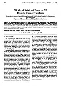
Fig. 1. Two views of the bounding box of the race car model with their associated depth-buffer images.

Our 3D shape retrieval system compares 3D models based on their visual similarity using depth lines extracted from depth images. The process first normalizes and scales 3D model into a bounding box. Then, it computes the set of N × N depth-buffer images associated to the six faces of the bounding box (see Fig. 1). The system then generates 2 × N depth lines per image, considering each depth image as a collection of N horizontal and N vertical depth lines. Finally, each

depth line is represented by a sequence of states using our proposed sequencing method (see Fig. 2). The shape descriptor consists in the set of 6 × 2 × N sequences. The sequence extraction process is described step by step in the following. 2.1. Pose Normalization A 3D object is generally given in arbitrary orientation, scale and position in the 3D space. As most of the 2D/3D shape descriptors do not satisfy the geometrical invariance, pose normalization is then necessary before the 3D object feature extraction. Some of the previous methods employed the Principal Component Analysis (PCA) as normalization step. PCA generates an alignment of a 3D-mesh model into a canonical coordinate system frame by translating, rotating, reflecting, and scaling the set of vertices. We have retained here the “Continuous” PCA [12] (CPCA) because it appears to be more complete and the most stable of all the approaches we have studied.

the visible points or “the attributes of pixels”, but rather considers the first derivative of the sequences. While there are sophisticated methods for estimating derivatives, we use the following estimate for simplicity D = dl(p) - dl(p + 1). This is the slope of the line segment between the depth at p and the depth at its right neighbor. To represent this estimate at each point, we introduce three states, Decreased, Increased and Constant, according to the sign of its derivative (negative or positive or null). We obtain information about the shape by considering the space derivative properties of the depth line.

2.2. Depth Lines Extraction The bounding box is used in rendering algorithms in order to generate depth-buffer images from a model. It is the minimal box, with the faces parallel to the coordinate hyper-planes that completely encompasses a 3D model. Each 3D model is projected perpendicularly on the planes of own bounding box, in order to generate six N × N depth-buffer images vi , i ∈ {1, ..., 6}. The rows and the columns of each image are decomposed into 6 × 2 × N depth lines of size N . 2.3. Sequencing of Depth Line The challenge of the sequencing method lies in the definition of states, which need to be efficient and robust representations of the shape information. It is possible to assimilate depth lines to 2D curves, thus the space points are taken as sequence elements. However, this sequencing technique has some disadvantages. When the depth line has several parts (e.g., contains disconnected background regions), there is a bad resolution in the matching process due to the fact that the dynamic programming algorithm matches empty samples. It is then interesting to discover, analyze and preserve the content of a depth line. The different regions present on a depth line are classified into two categories: Background regions: they represent the background of the projected plane. Sometimes, a 3D model might be rendered into several separated parts and also certain parts might contain holes. When the situation occurs, two types of background points can be rendered: interior points and exterior points. We want to distinguish these two background states in our sequencing. Projected object regions: they contain the projections of the visible points of 3D model. For these regions, we adopt a “derivative” description that does not consider the depths of

(a)

(b)

oooooo / -------- / \ --------- \ oooooo oooooo / -------- / - \ -------- \ oooooo oooooo / ------- // - \ -------- \ oooooo // --- \ / --- \ ccc // - \\ cc / ---- \ / --- \\ // --- \\ ccc / -- \ // - \\ / --- \ cc // --- \\ // --- \\ / \ cccc /// - \\ ccccc /\ // --- \\ // --- \\ cccccc /// - \\\ cccccc // --- \\ // --- \ cc / \ ccc /// - \\\ ccc / \\ c / --- \\ // --- \ ccc /\ cc /// - \\\ cc / \ ccc / --- \\ ooooooooooo / \ /// - \\\ / \ ooooooooooo //// - \\\\ oooooooooooo oooooooooooo oooooooooooo //// - \\\\ oooooooooooo ooooooooooo /// \ --- / \\ oooooooooooo ooooooooooo /// \ --- / \\\ ooooooooooo oooooooooo / -- /// - \\\ -- \ oooooooooo oooooooo / ----- // - \\\ --- \\ oooooooo ooooooo / --- ///// - \\\\\ --- \ ooooooo ooooooo / --- ///// - \\\\\ --- \ ooooooo oooooo / ---- ///// - \\\\\ --- \ ooooooo oooooo / ---- ///// - \\\\\ --- \ ooooooo oooooo / ---- ///// - \\\\\ --- \ ooooooo ooooooo / ---- //// - \\\\ ---- \ ooooooo ooooooo / ---- //// - \\\\ ---- \ ooooooo ooooooo // --- //// - \\\\ --- \\ ooooooo oooooooo // --- /// - \\\ -- \ - \ oooooooo / ---- \\ cc / - / - /// - \\\ - \ - \ cc / ----- \ / ----- \ ccc // -- // - \\ - \ - \ ccc / ----- \ / ----- \ / \ - \ - / - // - \ -- \ - / - / \ / ----- \ / ----- \ ccc / - / -- / - \ -- \ - \ ccc / ----- \ / ----- \ ccc / - / ------- \ - / \ cc / ----- \ / ---- \\ cc / -----------/ \ cc // ---- \ ooooooooo / -----------/ \ ooooooooo

(c)

/ ----- \ ccc / - / -- / - \ -- \ - \ ccc / ----- \ Fig. 2. (a). Depth image, (b). The horizontal sequences computed from the depth lines, (c). Sequencing of a depth line. Each depth line is encoded in a set of N states called sequence of observations. Each such observation is represented by one of the five characters, o, c, /, -, \ , representing the proposed states that compose the sequence: exteriorbackground, interior-background, increased-depth, constantdepth and decreased-depth (see Fig. 2.c). 3. 3D MODEL RETRIEVAL USING DYNAMIC PROGRAMMING For some sequence similarity matching, a very simple measure, such as Hamming distance, will suffice. It is the number of corresponding state positions that differ. However, this metric turned out not to be optimal in our sequence similarity computing. It is essentially due to the fact that two similar sequences often have approximately the same overall component shapes, but these shapes do not line up in X-axis. Thus, it is necessary to find the best alignment between two sequences before computing their similarity. As one can see on Fig. 3, the Hamming distance does not tolerate phase shifting of subsequences of the shape, thus, similar shapes that are not perfectly aligned along the X-axis lead to counter intuitive high distance values. To overcome

the limits of the Hamming metric, we introduce the Dynamic Programming distance to compare the shape descriptors, thus local deformations of objects’ boundaries can be matched. (a)

∆(O1, O2) =

6 X N −1 X X

DP D(S1i,j,k , S2i,j,k ).

(1)

i=1 j=r,c k=0

(b)

where i denotes the index of the rendered images, k the order of lines in the depth image, j indicates if the depth line is a row or a column and DPD is computed as in [15].

Fig. 3. Comparing the distances of two depth sequences by Hamming distance and dynamic programming distance while the sequences have an overall similar shape, but, they are not perfectly aligned along the X-axis. (a) 4 mismatches -·-·-, Hamming distance produces a pessimistic dissimilarity measure. (b) 2 mismatches -·-·-, a nonlinear alignment allows a more intuitive distance measure to be calculated.

3.1. Dynamic Programming In diverse domains, the dynamic programming has been developed to align two signals, two sequences or two series with different dynamics. While there are many algorithms in the literature, Dynamic Time Warping (DTW), NeedlemanWunsch algorithm and Smith-Waterman algorithm account for the majority of the literature. DTW has been well-adopted for curve alignment [13] and 2D shape matching [14]. The Needleman-Wunsch distance has already proven to yield superior performance for the retrieval of sequences, and we show that this is also the case for 3D shape matching. The Needleman-Wunsch algorithm [15], which calculates a “global” similarity distance between two sequences, has been used here. It computes the global alignments between two sequences, which produce the optimal score. Global scores require the alignment to begin at the beginning of each sequence and extend to the end of each sequence. To align two sequences, A = a0 a1 . . . aN −1 and B = b0 b1 . . . bN −1 using dynamic programming, we first construct a N -by-N match matrix M using the match operators (adjacent transposition C and substitution S) where the (ith ,j th ) element of matrix contains the similarity between sequences elements ai and bj . Then, we construct recursively the (N +1)by-(N + 1) matrix H (Fig. 4) using the match matrix M and the gap operators (insertion I or deletion D). When N = 32, the computational cost of the Needleman-Wunsch algorithm is not prohibitive. 3.2. Measuring Similarity between two 3D Models To compare two 3D models O1 and O2, we generate, 12 × N observation sequences S1i,j,k and S2i,j,k from the six rendered images. Then, we compute the dynamic programming distance (DP D) between each sequence of model O1 and the corresponding sequence of model O2. Finally, the dissimilarity between a pair of 3D models, O1 and O2, are computed as the sum of all DP Ds. Therefore, it is defined as follows:

|

-12 -9 -6 -3

0

3

6

\

-11 -8 -5 -2

1

4

7 10 13 16 19 18 17

9 12 15 18 18 20

\

-10 -7 -4 -1

2

5

8 11 14 17 16 15 14

|

-9 -6 -3

0

3

6

9 12 15 14 13 12 11

|

-8 -5 -2

1

4

7 10 13 12 11 10

9

8

|

-7 -4 -1

2

5

8 11 10

9

8

7

6

5

/

-6 -3

0

3

6

9

8

7

6

5

4

3

2

/

-5 -2

1

4

7

6

5

4

3

2

1

0 -1

/

-4 -1

2

5

4

4

3

2

1

0 -1 -2 -3

|

-3

0

3

2

2

1

3

2

1

0 -1 -2 -3

/

-2

1

1

3

2

1

0 -1 -2 -3 -4 -5 -6

/

-1

2

1

0 -1 -2 -3 -4 -5 -6 -7 -8 -9

0 -1 -2 -3 -4 -5 -6 -7 -8 -9-10-11-12 /

-

/

/

/

-

-

-

\

\

\

-

Fig. 4. Matching of the two observation sequences corresponding to the depth lines of Fig. 3 using Needleman-Wunsch algorithm [15].

4. EXPERIMENTAL RESULTS We made our tests on the Test Princeton 3D Shape Benchmark database [2] (907 models categorized within 92 distinct classes). The experimental results presented here were obtained with the following parameters: N = 32 for the different rendered image size; (C, S, I, D) = (−2, 1, 1, 1) for Needleman-Wunsch Algorithm. To compare objectively the retrieval effectiveness of the proposed approaches, we compute Precision-Recall diagrams commonly used in information search (the query is not counted in the answer as in [11]) and four quantitative measures for evaluating query results (see [2] for a description of this measures): (1) The Nearest Neighbor (NN), (2) The First Tier (FT), (3) the Second Tier (ST), (4) The Discounted Cumulative Gain (DCG). In Fig. 5, we compare our approach against the original depth buffer-based approach (DBA [11]) and in Fig. 6 we show some examples. Our method DLA clearly outperforms the DBA. When using the Hamming distance, our method based on the sequencing of depth lines provides more accurate retrieval results than the DBA, and by introducing the dynamic programming distance, the performance gain is increased. Moreover, if we compare these measures with the results listed in table 4 of [2], our approach produces 1%, 1.5%,

1.5% and 1% better than the top ranked Light Field Descriptor (LFD) [6], in term of NN, FT, ST and DCG measures.

[1] J.W.H. Tangelder and R.C. Veltkamp, “A survey of content based 3D shape retrieval methods,” in SMI’04, Genova, Italy, June 2004, pp. 145–156.

Test Princeton Database [907 models] 1

DLA−DPD [66.70 39.49 50.21 65.31] DLA−HD [61.52 35.94 45.63 62.13] DBA [59.21 32.48 41.67 58.88]

0.9 0.8

[2] P. Shilane, P. Min, M. Kazhdan, and T. Funkhouser, “The Princeton shape benchmark,” in SMI’04, Genova, Italy, June 2004, pp. 167–178.

0.7

Precision

6. REFERENCES

[3] T. Zaharia and F. Prˆeteux, “3D versus 2D/3D shape descriptors: A comparative study,” in SPIE Conf. on Image Processing: Algorithms and Systems, San Jose, CA, USA, Jan. 2004, vol. 5298.

0.6 0.5 0.4 0.3

[4] B. Bustos, D. A. Keim, T. Schreck, and D. Vranic, “An experimental comparison of feature-based 3D retrieval methods,” in 3DPVT’04, Thessaloniki, Greece, Sept. 2004.

0.2 0.1 0 0

0.1

0.2

0.3

0.4

0.5

0.6

0.7

0.8

0.9

1

Recall

Fig. 5. Average Precision-recall curves using the proposed depth line-based approach DLA (with dynamic programming distance DPD and Hamming distance HD) and the depth buffer-based approach DBA (with the same bounding box and 6 views). The mean NN, FT, ST and DCG values are given in the legends. 5. CONCLUSION In this paper, we have presented a new 3D descriptor based on depth lines and an associated similarity measure using dynamic programming. We have evaluated its performances on the Princeton Shape Benchmark database. The depth-line approach has proved to be efficient in space and accuracy for 3D retrieval, even if it used with the Hamming distance. Work in progress includes the test of other dynamic programming algorithms and other values of N to obtain an optimal ratio time/accuracy.

[5] A. Del Bimbo and P. Pala, “Content-based retrieval of 3D models,” ACM Trans. Multimedia Comput. Commun. Appl., vol. 2, no. 1, 2006. [6] D.Y. Chen, X.P. Tian, Y.T. Shen, and M. Ouhyoung, “On visual similarity based 3D model retrieval,” Computer graphics forum, vol. 22, no. 3, pp. 223–232, Sept. 2003. [7] T. Filali Ansary, M. Daoudi, and J-P. Vandeborre, “3D model retrieval based on adaptive views clustering,” in ICAPR’05, Bath, UK, Aug. 2005. [8] S. Mahmoudi and M. Daoudi, “3D models retrieval by using characteristic views,” in ICPR’02, Qu´ebec, Canada, Aug. 2002, pp. 11–15. [9] R. Ohbuchi, M. Nakazawa, and T. Takei, “Retrieving 3D shapes based on their appearance,” in MIR’03, Berkeley, CA, USA, Nov. 2003. [10] M. Chaouch and A. Verroust-Blondet, “Enhanced 2D/3D approaches based on relevance index for 3D-shape retrieval,” in SMI’06, Matsushima, Japan, June 2006. [11] D.V. Vranic, 3D Model Retrieval, Ph.D. thesis, U. of Leipzig, 2004. [12] D. Vranic, D. Saupe, and J. Richter, “Tools for 3D-object retrieval: Karhunen-Loeve transform and spherical harmonics,” in 2001 Workshop Multimedia Signal Processing, Cannes, France, Oct. 2001. [13] Kongming Wang and Theo Gasser, “Alignement of curves by dynamic time warping,” The Annals of Statistics, vol. 25, no. 3, pp. 1251–1276, 1997. [14] Eamonn J. Keogh, Li Wei, Xiaopeng Xi, Sang-Hee Lee, and Michail Vlachos, “Lb_ keogh supports exact indexing of shapes under rotation invariance with arbitrary representations and distance measures.,” in VLDB, 2006, pp. 882–893.

Fig. 6. Examples of similarity search. For each query, we show the top 5 objects matched with DLA approach. The similarities between the query models and the retrieved models are given below corresponding images. X and x indicate that the retrieved models belong or don’t belong to the query’s class, respectively.

[15] S. Needleman and C. Wunsch, “A general method applicable to the search for similarities in the amino acid sequence of two proteins,” Journal of Molecular Biology, vol. 48, no. 3, pp. 443–453, 1970.