3D CAD Model Retrieval Based on Multiple Levels of Detail Jiantao Pu Subramaniam Jayanti Suyu Hou Karthik Ramani* PRECISE, School of Mechanical Engineering, Purdue University, U.S.A.
Abstract This paper describes a new 3D model retrieval approach, which represents a 3D shape at three distinct levels of detail: contour level, silhouette level, and drawing level. This 3D-to-2D representation is supported by a 3D pose determination algorithm; to compute the similarity between 2D shapes at these levels, a combination of two different 2D shape descriptors is used to achieve a better performance. In addition, the results from the three levels were combined in five different schemes for obtaining the final ranked retrieval. In the prototype system, users can adjust the weights and interact with the different views and levels to emphasize the search intent more precisely. Based on average precision, the combination of the methods achieved 6-8% improvement over the individual levels. The proposed method which uses only three orthogonal views also performs comparably (avg. precision of 50.24%) with respect to the current best Light Field Descriptor method (50.68%).
1. Introduction In the past decades, a large amount of 3D models have been accumulated in the engineering domain. Reusing and sharing the knowledge embedded in these models is becoming an important way to accelerate the design process, improve product quality, and reduce costs. Generally, the term ‘similar models’ is meant for objects that are globally similar, but still have some differences in specific features. Therefore, a good search strategy for a 3D retrieval system should not only consider the global but also the local shape comparison between 3D models. Meanwhile, efficient query interfaces are also critical for engineering applications. For this purpose, the search engines introduced in [1, 2] support sketch-based user interfaces.
* Corresponding author {
[email protected]}
In our research, we use three orthogonal views (front view, side view and top view) to represent a 3D model. The query can be a 2D sketch, legacy drawing or a 3D model [23, 30, 27]. In a benchmark study that evaluated 13 different shape representation methods, Iyer et al. [33] found that the view-based methods showed better retrieval performance. In a similar study Shilane et al. [22] showed that light field descriptor (LFD), another view-based approach, achieved the best performance. In this study we extend the orthogonal view-based 3D similarity approach presented in [23] by splitting the information in each view into three distinct levels of detail – silhouette, contour and drawing level. We explore an engineering perspective of shape because engineering objects have high genus with several internal details and features, such as through and blind holes, which greatly affect the perceived similarity, as opposed to the global external shape. To the best of our knowledge such a multiple level of detail approach (MLD) has not been explored for similarity search with engineering objects. For comparing the effectiveness of the proposed MLD approach with existing approaches, we selected the 3D Spherical Harmonics (SH) [28], D2 shape distributions [16] and light field descriptor (LFD) [2] methods. In addition, we evaluated different schemes for combining the similarity obtained from the three levels of detail, by combining distances as well as ranks. Further we analyzed the effectiveness of each level and the combinations thereof for selected shape categories. The proposed approach has many advantages: (1) it requires only three orthogonal viewing directions, which is concurrent with engineering view of shape and design; (2) it allows users to sketch queries at any level of detail, thus supporting a coarse-to-fine search as well as searching with legacy 2D drawings; and (3) it has better retrieval performance (i.e., accuracy and efficiency) compared to several shape descriptors and comparable performance to the LFD.
2. Related work Traditionally, there have been several ways such as keyword-based search, encoding approach, and treelike structure navigation for users to perform information retrieval queries and facilitate product data reuse. Although these approaches are simple to implement, they are time-consuming and not sufficient to describe a 3D model. Design ideas can often be inferred from the geometric shape and reuse of existing designs in the form of CAD models provides several advantages for new product development such as reduced costs, quick development and production time and reduction in redundant effort. In the past several years, many methods were proposed to retrieve 3D models by measuring their shape similarity [32], several of which have been used in engineering CAD domain. There are two general approaches of representing 3D shape. The first approach develops shape descriptions directly from the 3D models (3D descriptors), while the second approach characterizes the 3D shapes using 2D views (View-based descriptors). View-based descriptors recognize 3D shapes from multiple 2D views in order to imitate humans’ uncanny ability to recognize objects from single or multiple views. For example, Cyr et al. [21] adopted a concept named aspect graph to represent a 3D object with a minimal set of 2D views. However, it has to determine the view transitions named “visual events” precisely; otherwise, a large number of views are needed. Funkhouser et al. [1] and Chen et al. [2] proposed algorithms in which the similarity between 3D models is converted to the similarity computation between 2D contours of the 3D models. The similarity between sketches and rendered silhouettes obtained from 3D objects is measured by a 2D analog of spherical harmonics representation. However, 13 and 10 thumbnail images from different directions are needed respectively. Also only contours and regions are considered in these methods. Therefore, significant information regarding (concave) shape features that occur frequently in engineering shapes, such as blind holes and cores, is lost. The shape representations for both 3D and 2D viewbased approaches can be further classified into Featurevector based and Topology based methods. (1) Feature-vector based methods. Shapes have been described in literature by several global geometric properties such as moment [9], tensors [10], density [11], symmetry [12], and other high-level shape features such as geons [13]. It is natural to use these features or their combinations to measure the similarity between 3D models since they can be computed
quickly for comparison. However, due to the fact that 3D shapes vary greatly, it is impossible to use limited number of features to describe a 3D shape. Several other methods describe shapes in much more detail using additional properties of the shape such as distributions of inter-point distances and angles [16], distributions of surface normals [7, 15], curvatures [48]. Other methods represent the 3D shape using distributions of distances from centroid or number of voxels along different regions in space (e.g. octants, concentric spheres, or sectors of a sphere) [14, 47]. Compared with several other methods, these statistical methods are not only fast and easy to implement, but also have some desired properties for practical applications, such as robustness and invariance. However, these methods are not sufficient to distinguish similar objects with obvious local differences due to the fact that local shape features are not depicted explicitly. (2) Topology-based methods. Besides the geometric and physical properties, the topology structure is important information for a 3D shape because human shape perception is partly based on structural decomposition [17]. Topology-based methods have many desired properties, such as intuitiveness, invariance, generality, and robustness. Global features and local features are depicted in the form of a skeleton. It is convenient for users to specify the desired part that they would like to match. However, despite the great advances made in the area of 2D and 3D shape decomposition, such as Hilaga et al.’s Multi-resolution Reeb Graphs (MRGs) [18], Siddiqi et al.’s shock graph [19], and Sundar et al.’s skeleton graph [20], it is still difficult to compute the topology in a robust and uniform way. In addition, several schemes for combining different features have been explored for content-based image retrieval [43, 45]. Recently, several methods for automatic feature combination and selection have also been successfully applied to 3D model retrieval [37, 40, 44, and 46].
3. Multiple Levels of Detail representation The multi-view, multiple level of detail approach described in this paper falls among the feature vectorbased methods with 2D views, and was inspired by several factors arising from traditional engineering knowledge and from a well-known fact that the human visual perception of a shape is organized from coarseto-fine details [3, 4-5]. Three orthographic drawings are widely used and have historically played an important role in engineering and technology and have been used for reconstruction and manufacturing 3D objects [35].
From an engineering graphics viewpoint, deciding the best view is an important step in obtaining multiview drawings. Generally in order to get the best views, the object must be positioned within an imaginary glass box such that the surfaces of major features are either perpendicular or parallel to the glass planes. The goal of this step is to create views with a minimum number of hidden lines and to draw the view of an object in its most natural position. Multi-view drawings provide the most accurate description of three-dimensional objects and structures for engineering and manufacturing requirements [39]. In order to produce a new product, it is necessary to know its true dimensions. Since engineering and technology depend on exact size and shape descriptions for designs, the best approach is to use orthographic projections to create views that show only two of the three dimensions (width, height, depth). Significant research has also been conducted in reconstructing 3D models from 2D orthographical views. Although this process is easy for humans with training to perform, several studies [34-36] aimed at automating 3D reconstruction from orthographic views indicate that 2D orthographic drawings contain sufficient shape information to represent the 3D models. In addition, current manufacturing practice still relies on the use of 2D drawings for interpretation and decision-making, making 2D drawings an integral part of the current product development processes. Hence, an orthogonal view-based approach to shape representation lends itself to easy interpretation, understanding, and interaction for engineering applications. To obtain such 2D orthographic views, the following steps were involved: (1) a pose determination method by finding three orthogonal
orientations with the maximum virtual contact area (VCA) [23] and (2) a drawing-like view generation method [23]. Comparison of the pose determination using VCA and PCA are shown in [23]. Along the three orientations, the projected views have a good accordance with the three main views concept (i.e., top view, front view and side view) in engineering graphics.
3.1. MLD Computation Table 1. shows an example of the proposed MLD representation of a 3D shape. The contour level reflects the global shape by which a user can “guess” the true object to some extent. The silhouette level conveys additional shape details using a few more additions to the contour level view. When the detailed shape information is not important, the silhouettes are enough to differentiate two similar objects with a higher confidence than the contour level. The third level contains the complete information, including the visual appearance and the occluded structure, using which a user can determine its shape precisely. Because of the intricate shape of engineering objects, we consider complete details in the third level. At the contour level, there are three different views along the principal axes; at the silhouette level, there are six different views; and at the full level, we use the three traditional drawinglike views along the principal axes to represent the drawing level. Below we will describe the algorithms to generate these views.
Table 1: MLD based Representation 3D Model
Contour Level
Silhouette Level
Drawing Level
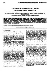
3.1.1. Contour Level. To obtain the shape at the contour level, the 3D model is projected along the intended directions by setting the z-value of each polygon to zero and rendering it in image space. In implementation, this operation can be efficiently completed with the help of any classic algorithm such as Painter’s Algorithm or the Z-buffer Algorithm. 3.1.2. Silhouette Level. A silhouette edge connects two polygons, one of which faces toward the viewer and the other facing away from the viewer. When a 3D object is projected onto a 2D viewing plane, its visual appearance is formed by all its silhouette edges. The efficient extraction of silhouettes has been widely studied in many applications ranging from computer vision to non-photorealistic rendering. Earlier hidden line removal methods [24] have been used to get the silhouette edges. Recent methods render the silhouettes of 3D models in image space include [25, 26]. In our application, we propose a method by which the silhouettes of a 3D model are efficiently generated in object space instead of image space. Figure 1 shows the process of silhouette generation.
Figure 1: Four steps for silhouette generation: (a) an original 3D model; (b) the result after backface culling operation; (c) the result after inside face culling operation; (d) the view without occlusion culling (Drawing Level); and (e) the silhouette view of (a). The first step is culling backward polygons [42]. Our contribution in this step is in improving the efficiency of the second step of discarding the insideedges. The inside-edge has a distinguishing property: it is shared by two polygons. With this definition, we can cull the inside-edges completely by traversing all the triangles with the help of a look-up table. The look-up table is an m×m matrix, where m is the number of remaining vertices after backface culling. The element (i, j ) represents the edge formed by vertices i and j. First, we can code all vertices from 0 to m - 1 . Then by traversing the 3D model after backface culling, we can fill this table according to the connecting relationship of the edges. Finally, the inside-edges are determined by checking whether the element at (i, j ) is filled more than twice. In practice, to save memory, we can use bits to represent the table. Figure 1(c) shows the inside-
edge culled result. The computational complexity of the look-up table method is O(n+m). The third step is projecting the result after the inside-edge culling operation along the respective orientation. In order to render the silhouette the occluded structure is culled by executing a series of fast ray-triangle intersection tests. The final 2D view is obtained by projecting the remaining polygons onto the corresponding projection planes.
3.1.3. Drawing Level. We perform all the steps from silhouette extraction (Section 3.1.2), except occluded edge culling, to obtain the drawing level views, which contain the complete shape information.
3.2. Shape Description While pose determination is the process of registering the viewing direction of similar objects, we still need a shape descriptor with rotation invariance for registering the 2D geometric shapes no matter how they are rotated in object space. After view-generation, the 2D views thus obtained are represented using two different shape descriptors – 2.5D Spherical Harmonics [27] and 2D Shape Histogram [27]. Dissimilarity between a pair of 2D views is obtained as a linear sum of dissimilarities from these two shape descriptors. Given a pair of 3D objects (i.e. two sets of 2D views), the pair of 2D views which provide the best match (i.e. with the least dissimilarity) are the principal matching view pair. The other two matching view pairs are determined likewise from the remaining views. The total dissimilarity between two 3D models is obtained through the summation of dissimilarity between the three sets of matching view pairs. Each view is represented by a feature vector obtained from 2DSH and 2.5DSH methods. For 2DSH method the feature vector is a histogram of pairwise distances, and for 2.5DSH the feature vector is a set of spherical harmonics coefficients as described in [27]. For two feature vectors H1 and H2, the similarity S is given by:
S ( H1 , H 2 ) = Ln ( H1 , H 2 ) =
h
n
∑ ( H (i ) − H 1
2
(i )) n
(1)
i =0
where h is the number of bins in the histogram. Each of these feature vectors are used with the different levels of detail, unlike in [27] where they were used only with the drawing level.
4. Combination of Multiple Levels in MLD Due to the complex nature of “3D shape,” it is difficult to find different methods that can describe a
3D shape in a consistent way. Since the three levels of the MLD representation emphasize different aspects of the shape we expect it to emphasize different aspects of perceived shape similarity. Although, the three levels can be combined in many different ways [40, 45-46], we studied four different ways of combining the levels – Linear Weighted Sum (LWS), Minimum distance (MIN), Average Rank (AR), and Minimum Rank (MR). Note that we combined the distances obtained from the three levels of detail for LWS and MIN, while we use the ranks for AR and MR methods.
4.1. Linear Weighted Sum (LWS) Given a query object Q and a database object D, the final dissimilarity d(Q, D) , using the three levels is expressed as: (2) d(Q,D) = wL1 L1 (Q,D)+ wL2 L2 (Q,D)+ wL3 L3 (Q,D)
譫
譫
譫
where d L1 , d L2 , and d L3 are the dissimilarities (distances) between A and B at the three levels of detail, and wL1 , wL 2 ,and wL3 are the weights values given to the respective levels. Higher weight value means that the corresponding level plays a more important role in the final dissimilarity, d(Q, D) . Weight estimation by brute force: We performed tests to determine the effect of the level weights ( wL1 , wL 2 ,and wL3 ) on the search performance as reflected in the PRCs. Since these weights were normalized to yield a sum of 1.0, there are only two independent weights ( wL1 , wL 2 ), the third weight ( wL3 = 1- wL1 - wL 2 ) being dependent on the values of the first two. The value of the two weights wL1 and wL 2 were systematically changed from 0.0 to 1.0. Weight estimation by heuristic rule: We adopted a heuristic rule to obtain the weights for the individual levels in the MLD. By employing 25% of the database as the training set we obtained the average precision for each level of detail (Pi, i=1...3). The average precision was calculated for a retrieval size of 30. The precision values indicate the confidence level of the different MLD levels. Hence, we used the following rule to obtain weights (wi) for the individual levels: wi = Pi /(P1 + P2 + P3 ) .
4.2. Minimum Distance (MIN) In this approach, for a given query the minimum value among the dissimilarities at the three levels between the query object and the data object is assigned as the final similarity.
d(A,B) = min ( d L1 (A,B),d L2 (A,B),d L3 (A,B))
(3)
4.3. Average Rank (AR) While the LWS and MIN methods combine the levels based on a distance measure, this approach is based on average rank. For each query object Q, we store the results retrieved using the three levels into three sorted lists R1, R2, R3, respectively. For each object D in the database, we calculate the average rank for this object from the three sorted lists. The final result for the query is the list of database objects sorted with respect to this average rank value. In essence, each search criterion (i.e. dL1, dL2 and dL3) votes on the relevance of the database object D with respect to the query Q. The objects with the best average rank are shown in the top results.
4.4 Minimum Rank (MR) The minimum rank criterion is similar to the minimum distance criteria. However, we only consider the best rank obtained from any of the levels and use that for the final results.
5. 3D Model Retrieval In order to test the performance of the MLD method, we used the Engineering Shape Benchmark (ESB) database [33]. This database publicly available (http://www.purdue.edu/shapelab/) has 867 CAD models from various sources including some models from the industry. The benchmark consists of models grouped into 44 classes of similar parts which are available for download. Standard precision recall experiments were conducted by retrieving similar models from the database, using each model as a query. The curves were averaged over all the classes.
5.1. Search Performance The search time for a query in the prototype system is between 1 to 5 seconds depending on the size of the 3D model which ranges from 100 polygons to 100,000 polygons. Note that this time includes the time taken to generate the views for the query object and matching the feature vectors with the views of all the objects indexed in the database. The Precision-Recall (PR) curve is the most common way to evaluate the performance of a retrieval system. The computed precision recall curves for the MLD method were compared against existing shape descriptors, viz., 3D Shape Distributions (SD), Spherical Harmonics (SH)
and LFD. Detailed description of these methods is beyond the scope of this paper. In their recent work Iyer et al. [33] computed precision recall curves for 2.5D Spherical Harmonics (2.5DSH) and 2D Shape Histogram (2DSH) methods on a single level of detail which corresponds to the drawing level. Both these methods demonstrated consistently higher precision recall curves as compared to the other shape representations. Further, the 2.5DSH method performed better than the 2DSH method. Overall Performance 1
LFD MLD (LWS) 2.5DSH 2D SH SH SD
Precision
0.8 0.6 0.4 0.2 0 0
0.2
0.4
0.6
0.8
1
Recall
(a) Overall Performance
LFD Level 1 Level 2 Level 3 MLD (LWS) MLD (MIN) MLD (AR) MLD (MR)
1
Precision
0.8 0.6 0.4 0.2
Section 5.3. For the LFD method, we used the executable code available from (http://3d.csie.ntu.edu.tw). As shown in Figure 2(a), the precision recall curve for the MLD method is consistently higher than the 2.5DSH and 2DSH methods, especially at higher recall values. Figure 2 (b) shows that the performance of four different MLD approaches and also each of the levels of detail to be similar. Interestingly, they are all better than the other individual methods (viz. 2.5DSH and 2DSH) shown in Figure 2(a).
5.2 Results from Combining Multiple Levels From the results in Figure 2 and Table 2 we can see that, in general, the combination methods perform better than individual levels. Note that the 11 point average precision and R-precision values for the LFD and SD methods obtained from our experiments agree with those obtained in ref. [37] for the multimedia database. Figure 2(b) compares the precision recall curves for all combination methods used with MLD. Although different methods perform differently for various groups, certain trends are visible from the PR curves. For the LWS method, we found that the brute force approach yielded an optimal weight combination of (0.33, 0.33, 0.33) and found that it achieves the best performance among all combination methods, as indicated by the average precision and R-precision. It performed between 6-8% above the 2.5D SH and produced 3-4% increase in the average precision above the Level 3. Similarly, the heuristic method resulted in a similar weight combination of (0.33, 0.34, 0.33). This result suggests that the three levels are equally significant for the MLD method when evaluating the performance over the entire database of shapes. Table 2: Precision for different combination schemes
0 0
0.2
0.4
0.6
0.8
1
Recall
(b) Figure 2: Precision Recall curves for the MLD method and existing shape representations.
From our experiments in this study we found that the MLD method performs significantly better than all existing methods except LFD. With respect to LFD the average performance of MLD is similar, although for some classes (e.g. curved housings, nuts, bolt-like parts, T-shaped parts) MLD performs better and for many other classes (e.g. machined plates, L Blocks, Rocker Arms) LFD performs better. Hence, the results are also studied qualitatively for some representative classes in
Method SD SH 2D SH 2.5D SH MLD (Level 1) MLD (Level 2) MLD (Level 3) MIN AR MR LWS (Equal wts) LFD
Average 11 Point Precision Average (@ Ret = 30) Precision (%) (%) 15.79 29.36 26.63 38.59 27.51 40.60 28.94 42.08 31.33 46.57 31.56 46.84 31.31 46.90 32.74 48.10 32.60 49.09 33.24 49.10 35.75 50.24 34.59 50.68
R-Precision (%) 19.24 30.79 31.77 33.29 36.04 36.59 36.03 37.71 37.87 38.93 39.26 41.65
It should be noted that these results are obtained using the aggregated performance over the whole database. For individual classes, other weight combinations yield significantly better retrieval precision. For comparison between different methods we calculated the following performance measures (see Table 2): (a) The 11-point average precision at each point of recall, (b) precision after retrieval size (Ret.=) 30 objects, and (c) precision at retrieval size (Ret.=) R, where R is the relevant documents for the query [31].
objects with similar top view but with subtle difference in the side view are still shown as similar, as opposed to LFD which retrieves dissimilar objects that match with the query in other views.
5.3 Comparison with Light Field Descriptors The two view-based methods described in Section 3.3 were benchmarked against several existing methods by Iyer et al. [33]. These two methods were found to have performed significantly better than several existing 3D shape representations such as D2 Shape Distributions (SD) [16], and Spherical Harmonics (SH) [1, 28]. Note, however, that those two methods (viz., 2.5DSH and 2DSD) used the drawing level alone for comparison. In this paper, we present a comparison of our new MLD method with LFD as it has been shown to provide the best precision among several 3D shape representations evaluated by Shilane et al. [22]. The LFD method obtains 10 views of an object from each camera orientations and represents the views as images. The shape of the 2D views is described using Fourier Descriptors and Zernike moments [2]. When comparing two 3D objects all sets of 10 views obtained with each of the 60 different camera orientations are compared using these 2D shape descriptors. The best set of matching views (i.e. with minimum distance between 10 pairs of views) gives the similarity between the two objects. Hence, the final similarity is based on a several views of an object, compared to three orthogonal views used in our approach. The LFD approach has several advantages, because for many 3D objects such as those found in multimedia, it is difficult to obtain a robust pose, hence matching of several views will likely result in better precision. However, MLD method performs better than the LFD method when applied to several engineering objects possibly because of the 2D shape descriptors used for comparison and the details presented in the Silhouette and Drawing levels of the MLD. As a result, several false positives are introduced in the results for LFD when a large number of 3D objects have a common matching view but are different from other perspectives. For example, the LFD method retrieves only 10 of the 14 relevant objects (other than the query itself) in the top 20, for the query object shown in Figure 3(a), leading to a drop in precision at higher recall. Since the MLD method takes three views, all the
(a) T-shaped parts - LFD
(b) T-shaped parts - MLD (LWS)
(c) Prismatic Stock - LFD
(d) Prismatic Stock - MLD (LWS) Figure 3: Search results for parts from (a)-(b) “Tshaped” and (c)-(d) “Prismatic Stock” categories.
5.4. Results for Individual Shape Classes
Prismatic Stock 1
6. Conclusions and Future Work In this paper, we introduced a multiple level of detail (MLD) approach to 3D model retrieval. The key characteristics of the approach are: (1) a 3D model is
Precision
0.8 0.6
LFD Level 1 Level 2 Level 3 MLD (LWS) MLD (MIN) MLD (AR) MLD (MR)
0.4 0.2 0 0
0.2
0.4
0.6
0.8
1
Recall
(a) Spoked Wheels
LFD Level 1 Level 2 Level 3 MLD (LWS) MLD (MIN) MLD (AR) MLD (MR)
1
Precision
0.8 0.6 0.4 0.2 0 0
0.2
0.4
0.6
0.8
1
0.8
1
Recall
(b) T shaped parts 1 0.8 Precision
In order to gain more insight into the performance of the different levels and their combinations, we plotted the precision recall curves for individual classes from the ESB database. From the PR curves shown in Figure 4 we observe that the LFD method performs better than any level or combination of the MLD approach. For certain classes, the individual levels perform better than the combinations (e.g. Level 3 in Figure 4a and Level 1 in Figure 4b). While for many classes all the tested methods give similar PR curves, we present analysis of three classes where there is a wide variation in performances. 1. For “prismatic stock” category where all models are cubical with no other feature, the search at Drawing Level performs better than those on the other two levels. The reason for this trend is that from the information present in the contour level, there are a number of models where at least two views match, leading to a significant number of false positives. However, by adding more information about the internal structure in Levels 2 and 3, more relevant models are retrieved in the top search results, as seen in Figure 3c. In some cases, Drawing Level achieves better precision than the LFD method. 2. As opposed to its poor performance in “Prismatic Stock” category, the Contour Level (Level 1) achieves much higher precision than the other two levels for “Spoked Wheels” owing to the fact that this category is characterized by the external rim structure connected with spokes, which is encoded in Level 1. However, Levels 2 and 3 include additional detail which is not important for retrieving parts within this class. Note that both Level 1 and LFD perform better than all other methods. 3. Figure 4c shows one of the classes where the MLD method provides consistently higher precision values than the LFD method. At the same time we should note that the performance of the LFD method is comparably much better for this class reaching the ideal PR curves. In a total of 16 classes the LFD method shows better performance than the LFD method while for 10 other classes the MLD method provides consistently higher precision values. Representative results for the two methods on the “T-shaped parts” class in Figure 3a-b.
0.6
LFD Level 1 Level 2 Level 3 MLD (LWS) MLD (MIN) MLD (AR) MLD (MR)
0.4 0.2 0 0
0.2
0.4
0.6 Recall
(c) Figure 4: Precision recall curves for individual classes
represented by a few 2D views along three orthogonal directions; (2) these views are composed of three levels: contour level, silhouette level and drawing level, which represent the object with increasing level of detail; (3) different combinations of the levels provide specific benefits to certain shape classes based on user perception of similarity; and (4) the user is allowed to
combine the different levels based on search requirements. We evaluated different approaches for combining the search results, and found that a linear weighted sum (LWS) of distances achieves the best performance among all methods, as indicated by the average precision. This combination method performed between 6-8% above the individual levels. In spite of taking only three views, the MLD performs as well as the LFD method with 60 views for the engineering shapes considered here. From the 11point average precision values the two methods perform equally with 50.24% and 50.68% precision. The MLD method uses orthogonal views allowing the user to naturally interact with the search system. These results reinforce the fact that for engineering shapes three orthogonal views can be used in similarity search. In order to further improve the MLD approach, it may be desirable to use region-base descriptors such as Zernike moments for the views as done with LFD. In addition, emphasizing some views more than the others may improve the retrieval performance, since similarity can often be determined from a single view. One of the advantages of the MLD method over LFD method lies in the fact that by separating the information into the different views and levels, the user can place importance on different aspects of the shape in order to retrieve the desired results. For example, the user may search only using the Contour Level or the Silhouette level or interact with three views to express the search intent. Alternatively, the user can suggest the importance for the individual views as well.
7. Acknowledgements We like to acknowledge the support of National Science Foundation Grant (11S-0535156) from the information and intelligent systems.
8. References [1] T., Funkhouser, P., Min, M., Kazhdan, J., Chen, A., Halderman, D., Dobkin, and Jacobs, D.,“A Search Engine for 3D Models,” ACM Transactions on Graphics, 2003,22(1): pp.83-105. [2] D.Y., Chen, X.P., Tian, Y.T., Shen, and M., Ouhyoung, “On Visual Similarity Based 3D Model Retrieval,” Computer Graphics Forum (Eurographics’2003), 2003, 22(3): pp.223232. [3] P. G., Schyns. “Diagnostic Recognition: Task Constraints, Object Information, and Their Interactions,” Cognition, 1998, 67: pp.147-179. [4] D. M., Parker, J. R., Lishman, and J., Hughes, “Role of Course and Fine Spatial Information in Face and Object
Processing,” Journal of Experimental Psychology: Human Perception and Performance,1996, 22: pp.1448-1466. [5] T., Sanocki, “Interaction of Scale and Time during Object Identification,” Journal of Experimental Psychology: Human Perception and Performance, 2001, 27: pp.290-302. [6] M., Petrou, and P., Bosdogianni, Image Processing: The Fundamentals, John Wiley, 1999. [7] B., Horn, “Extended Gaussian Images”, Proc. IEEE 72, 12(12), pp.1671-1686. New Orleans, USA, 1984. [8] S.B., Kang, and K., Ikeuchi, “The Complex EGI: A New Representation for 3D Pose Estimation,” IEEE Transactions on Pattern Analysis and Machine Intelligence, 1993, 15(7). [9] M., Tal, A., Elad, and S., Ar, “Content Based Retrieval of VRML Objects: An Iterative and Interactive Approach,” Proc. 6th Eurographics Workshop on Multimedia 2001, Manchester, UK, 2001, pp.107-118. [10] M.T., Suzuki, “A Web-based Retrieval System for 3D Polygonal Models,” Proc. Joint 9th IFSA World Congress and 20th NAFIPS International Conference (IFSA/NAFIPS2001), Vancouver, 2001, pp.2271-2276. [11] C., Zhang, and T., Chen, “Indexing and Retrieval of 3D Models Aided by Active Learning,” Proc. ACM Multimedia 2001, Ottawa, Ontario, Canada, 2001, pp. 615-616. [12] M., Kazhdan, B., Chazelle, D., Dobkin, T., Funkhouser, and S., Rusinkiewicz, “A Reflective Symmetry Descriptor for 3D Models,” Algorithmica, 2003, 38(2): pp.201-225. [13] K., Wu, and Levine, M., “Recovering Parametric Geons from Multiview Range Data,” Proc. CVPR, 1994, pp.159– 166. [14] M., Ankerst, G., Kastenmuller, H.P., Kriegel, and T., Seidl, “3D Shape Histogram for Similarity Search and Classification in Spatial Databases,” Proc. 6th International Symposium on Spatial Databases, Hong Kong, China, 1999, pp.207-228. [15] E., Paquet, and M., Rioux, “Nefertiti: A Tool for 3-D Shape Databases Management,” SAE Transactions: Journal of Aerospace 108, 2000, pp.387–393. [16] R., Osada, T., Funkhouser, B., Chazelle, and D., Dobkin, “Shape Distribution,” ACM Transactions on Graphics, 2002, 21(4): pp.807-832. [17] I., Biederman, “Recognition-by Components: A Theory of Human Image Understanding,” Psychological Review, 1987, 94(2): pp. 115-147. [18] M., Hilaga, Y., Shinaagagawa, T., Kohmura, and T.L., Kunii, “Topology Matching for Fully Automatic Similarity Estimation of 3D Shapes,” Proc. SIGGRAPH 2001, Computer Graphics Proceedings, Annual Conference Series, Los Angeles, USA, 2001,pp.203–212. [19] K., Siddiqi, A., Shokoufandeh, S., Dickinson, and S., Zucker, “Shock Graphs and Shape Matching,” Computer Vision, 1999, 35(1): pp.13-20. [20] H., Sundar, D., Silver, Gagvani, and S., Dickinson, “Skeleton Based Shape Matching and Retrieval,” Shape Modeling International 2003, Seoul, Korea, 2003, pp.130142.
[21] C.M. , Cyr, and B.B., Kimia, “3D Object Recognition Using Shape Similarity-Based Aspect Graph,” Proc. 8th International Conference on Computer Vision, Vancouver, Canada, 2001, pp.254-261. [22 P.,] Shilane, P., Min, M., Kazhdan, and T., Funkhouser, “The Princeton Shape Benchmark,” Proc. Shape Modeling International 2004, Genova ,Italy, 2004, pp.167-178. [23] J.T. , Pu, and K., Ramani, “An Automatic Drawing-like View Generation Method from 3D Models”, Proc. ASME IDETC/CIE Conference, Long Beach, CA, September 24-28, 2005. [24] A., Appel, “The Notion of Quantitative Invisibility and the Machine Rendering of Solids,” Proc. ACM National Conference 1967, Washington D.C., 1967, pp.387-393. [25] L., Markosian, M.A., Kowalski, S.J., Trychin, L.D., Bourdev, D., Goldstein, and J.F., Hughes, “Real-time Nonphotorealistic Rendering,” Proc. SIGGRAPH, 1997, pp.415420. [26] R., Raskar, and M., Cohen, “Image Precision Silhouette Edges,” Proc. of Symposium on Interactive 3D graphics, Atlanta (USA), 1997, pp.415-420. [27] J.T., Pu, and K., Ramani, “On Visual Similarity based 2D Drawing Retrieval”, Computer-Aided Design, 38, 2006, pp. 249–259. [28] M., Kazhdan, T., Funkhouser, and S., Rusinkiewicz, “Rotation Invariant Spherical Harmonic Representation of 3D Shape Descriptors,” In Proceedings of the Eurographics/ACM SIGGRAPH Symposium on Geometry Processing, Aachen, Germany, 2003,pp.156-164. [29] D., Healy, P., Kostelec, S., Moore, “FFTs for the 2Sphere--Improvements and Variations,” Journal of Fourier Analysis and Applications, 2003, 9(4): pp.341–385. [30] J.T., Pu, and K., Ramani, “A 2D Sketch User Interface for 3D CAD Model Retrieval,” Journal of Computer Aided Design and Application, 2005, 2(6):pp.717-727. [31] C. K. van Rijsbergen. Information Retrieval. Butterworths,1975. [32] J. W., Tangelder, and R. C., Veltkamp, “A survey of content based 3D shape retrieval methods.” In Proc. Shape Modeling International, Genoa, Italy, 2004, pp.145-156. [33] N., Iyer, S., Jayanti, and K., Ramani, “An Engineering Shape Benchmark for 3D models,” Proc. of ASME IDETC/CIE 2005, Long Beach, CA, September 24-28, 2005. [34] K.-Z. Chen, and X.-A., Feng, “Solid model reconstruction from engineering paper drawings using Genetic Algorithms”, Computer-Aided Design, 2003, 35(13): pp. 1235-1248. [35] W., Geng, J., Wang, and Y., Zhang, “Embedding visual cognition in 3D reconstruction from multi-view engineering drawings”, Computer-Aided Design, 2002, 34, pp. 321-336 [36] H., Lee, and S., Han, “Reconstruction of 3D interacting solids of revolution from 2D orthographic views,” ComputerAided Design, November 2005, 37(13): pp. 1388-1398. [37] R., Ohbuchi, and Y., Hata, “Combining Multiresolution Shape Descriptors for 3D Model Retrieval,” Proc. WSCG 2006, Plzen, Czech Republic, Jan. 30-Feb. 3, 2006.
[38] S.-H., Guan, M.K, Hsieh, C.C., Yeh, and B.-Y., Chen, “Enhanced 3D Model Retrieval System through Characteristic Views using Orthogonal Visual Hull.” ACM SIGGRAPH 2004 Conference, Los Angeles, California, USA, 2004. [39] G.R., Bertoline, E.N., Wiebe, Fundamentals of Graphics Communications, Fourth Edition, McGraw Hill, 2005, pp 191-220 [40] I., Atmosukarto, W.K., Leow, and Z., Huang, “Feature Combination and Relevance Feedback for 3D Model Retrieval, Proc. 3DPVT. 2005, pp. 334-339. [41] H. Zhang, and K.E., Hoff, “Fast Backface Culling using Normal Masks,” In Proceedings of the 1997 symposium on Interactive 3D graphics, Rhode Island (USA), 1997, pp.103106, [42] N., Iyer, S., Jayanti, K., Lou, Y., Kalyanaraman, and K., Ramani, “Three Dimensional Shape Searching: State-of-theart Review and Future Trends,” Computer-Aided Design, April 2005, Volume 37, Issue 5, 15 pp. 509-530. [43] R.D.S., Torres, A.X., Falcão, B., Zhang, W., Fan, E.A., Fox, M.A., Gonçalves, and P., Calado, “A new framework to combine descriptors for content-based image retrieval.” CIKM 2005: pp. 335-336. [44] B., Bustos, D., Keim, D., Saupe, T., Schreck, and D., Vranić, “Automatic Selection and Combination of descriptors for Effective 3DSimilarity Search,” Proc. IEEE MCBAR'04, pp. 514- 521, (2004). [45] D., Heesch, and S.M., Rüger, “Combining Features for Content-Based Sketch Retrieval - A Comparative Evaluation of Retrieval Performance.” ECIR 2002: pp. 41-52. [46] Leifman, G., Meir, R. and Tal., “A. Semantic-Oriented 3D Shape Retrieval using Relevance Feedback”, The Visual Computer (Pacific Graphics), October 2005, Volume 21, Numbers 8-10, pp.865-875. [47] Vranic, D.V., “An improvement of rotation invariant 3D-shape descriptor based on functions on concentric spheres”, ICIP 2003, 2003, 3, pp. 757-760. [48] Zaharia, T., and Preteux, F., “3D shape-based retrieval within the MPEG-7 framework,” In SPIE Conf. on Nonlinear Image Processing and Pattern Analysis XII, January 2001, Volume 4304, pp 133-145.