from bottom to top, segment fragments of increasing size are detected. These fragments ... on a Pentium III laptop. Our method uses the segmentation by weighted aggre- ... operators for multiscale edge detection [10, 14]. These op- erators are ...
Segmentation and Boundary Detection Using Multiscale Intensity Measurements Eitan Sharon, Achi Brandt�, Ronen Basriy Dept. of Computer Science and Applied Math The Weizmann Inst. of Science Rehovot, 76100, Israel Abstract Image segmentation is difficult because objects may differ from their background by any of a variety of properties that can be observed in some, but often not all scales. A further complication is that coarse measurements, applied to the image for detecting these properties, often average over properties of neighboring segments, making it difficult to separate the segments and to reliably detect their boundaries. Below we present a method for segmentation that generates and combines multiscale measurements of intensity contrast, texture differences, and boundary integrity. The method is based on our former algorithm SWA, which efficiently detects segments that optimize a normalized-cutlike measure by recursively coarsening a graph reflecting similarities between intensities of neighboring pixels. In this process aggregates of pixels of increasing size are gradually collected to form segments. We intervene in this process by computing properties of the aggregates and modifying the graph to reflect these coarse scale measurements. This allows us to detect regions that differ by fine as well as coarse properties, and to accurately locate their boundaries. Furthermore, by combining intensity differences with measures of boundary integrity across neighboring aggregates we can detect regions separated by weak, yet consistent edges.
1 Introduction Image segmentation methods divide the image into regions of coherent properties in an attempt to identify objects and their parts without the use of a model of the objects. In spite of many thoughtful attempts, finding a method that can produce satisfactory segments in a large variety of natural images has remained difficult. In part, this may be due to the complexity of images. Regions of interest may differ from surrounding regions by any of a variety of properties, and these differences can be observed in some, but often not in all scales. In this paper we take a step toward a better seg� Research supported in part by the Carl F. Gauss Minerva Center for Scientific Computation at the Weizmann Institute of Science. y Research was supported in part by the Minerva Grant, by the Israeli Ministry of Science, Grant No. 2104, and by the European Commission Project IST-2000-26001 VIBES.
mentation algorithm. Our method is based on the segmentation algorithm presented in [22]. It uses the multiscale structure built by this algorithm to measure and incorporate various properties such as intensity contrast, isotropic texture, and boundary integrity. This results in an efficient algorithm that detects useful segments in a large variety of natural images. We demonstrate the quality of our segmentations by comparing them to segmentations obtained with other state-of-the-art algorithms [23, 22]. Segments that differ by coarse scale properties introduce a specific difficulty to the segmentation process. Since initially we do not know the division of the image into segments, any coarse measurement must rely on an arbitrarily chosen set of pixels (“support”) that may often include pixels from two or more segments, particularly near the boundaries of segments. This may lead to significant oversmoothing of the measured properties and to blurring the contrast between segments, inevitably leading to inaccuracies in the segmentation process. On the other hand, since segments often differ only by coarse scale properties, such segments cannot be detected unless coarse measurements are made. Our method attempts to solve this “chicken and egg problem.” It does so by building a pyramid structure over the image. The structure of the pyramid is determined by the content of the image. As the pyramid is constructed from bottom to top, segment fragments of increasing size are detected. These fragments are used as a support area for measuring coarse scale properties. The new properties are then used to further influence the construction of larger fragments (and eventually whole segments). By measuring properties over fragments we avoid the over-smoothing of coarse measurements (as can be seen in Figure 1), and so segments that differ in coarse scale properties usually stand out. Our experiments demonstrate a considerable improvement over existing approaches. The process is very efficient. The runtime complexity of the algorithm is linear in the size of the image. Our implementation (whose runtime may still be significantly reduced) applied to an image of 200 � 200 pixels takes about 5 seconds on a Pentium III laptop. Our method uses the segmentation by weighted aggre-
ISBN 0-7695-1272-0/01 $10.00 (C) 2001 IEEE
gation (SWA) due to [22] as a framework for the process. This algorithm uses techniques from algebraic multigrid to find the segments in the image. Like other recent segmentation algorithms [26, 23, 8, 25] the method optimizes a global measure, a normalized-cut type function, to evaluate the saliency of a segment. To optimize the measure, the algorithm builds an irregular pyramid structure over the image. The pyramids maintains fuzzy relations between nodes in successive levels. These fuzzy relations allow the algorithm to avoid local decisions and detect segments based on a global saliency measure. Pyramids constructed over the image have been used for solving many problems in computer vision (e.g., [3, 6, 24]). Typically, the image is sampled at various scales and a bank of filters is applied to each sampling. Segmentation is generally obtained by going down the pyramid and performing split operations. Subsequent merge operations are applied to reduce the effect of over-segmentation (e.g., [12, 17, 1, 2, 19]). Over-smoothing introduces a serious challenge to these methods. A different kind of pyramid structure is built by agglomerative processes (see [9, 7]). These processes, however, are subject to local, premature decisions. Other approaches that attempt to reduce the problem of over-smoothing include the use of directional smoothing operators for multiscale edge detection [10, 14]. These operators are local and require an additional process for inferring global segments. Also of relevance are methods for smoothing using unisotropic diffusion [4, 18, 20]. These methods avoid over-smoothing, but typically involve a slow, iterative process that is usually performed in a single scale. In Section 2 we briefly review the SWA algorithm. Later, in Section 3 we describe how to involve integral measures over a segment in the segmentation process. We demonstrate this with two measures, the average intensity of a segment and its variance across scale. In Section 4 we discuss how to introduce and use boundaries in the segmentation process. Finally, we show experiments in Section 5.
2 Overview of the SWA Algorithm [22] introduced an efficient multiscale algorithm for image segmentation. In this algorithm a 4-connected graph G = (V; E; W ) is constructed from the image, where each node vi 2 V represents a pixel, every edge eij 2 E connects a pair of neighboring pixels, and a weight wij is associated with each edge reflecting the contrast in the corresponding location in the image. The algorithm detects the segments by finding the cuts that approximately minimize a normalized-cut-like measure. This is achieved through a recursive process of weighted aggregation, which induces a pyramid structure over the image. This pyramid structure is used in this paper to define geometric support for coarse scale measurements, which are then used to facilitate the
segmentation process. In this section we briefly describe the SWA algorithm. We note that we make two slight modifications relative to its original implementation. First, we change the normalization term in the optimization measure. We normalize the cost of a cut by the sum of the internal weights of a segment rather than by its area. Thus, our measure is related to that used in [23]. Secondly, we initialize the graph with weights that directly reflect the intensity difference between neighboring pixels, rather than using the “edgeness measure” defined in [22]. Specifically, we use wij = e �jIi Ij j , where Ii and Ij denote the intensities in two neighboring pixels i and j , and � > 0 is some constant. The SWA algorithm proceeds as follows. With every segment S = fs1 ; s2 ; :::; sm g � V we associate a state vector u = (u1 ; u2 ; :::; un ) (n = kV k), where
ui =
�
1 0
if if
i2S i 2= S:
(1)
The cut associated with S is defined to be
E (S ) =
X i6=j
wij (ui uj )2 ;
(2)
and the internal weights are defined by
N (S ) =
X
wij ui uj :
(3)
The segments that yield small (and locally minimal) values for the functional
(S ) = E (S )=N (S );
(4)
for some predetermined constant > 0, and whose volume is less than half the size of the image, are considered salient. The objective of the algorithm is to find the salient segments. To this end a fast transformation for coarsening the graph was introduced. This transformation produces a coarser graph with about half the number of nodes (variables), and such that salient segments in the coarse graph can be used to compute salient segments in the fine graph using local processing only. This coarsening process is repeated recursively to produce a full pyramid structure. The salient segments emerge in this process as they are represented by single nodes at some level in the pyramid. The support of each segment can then be deduced by projecting the state vector of the segment to the finest level. This segmentation process is run in time that is linear in the number of pixels in the image. The coarsening procedure proceeds recursively as follows. We begin with G[0] = G. (The superscript denotes the level of scale.) Given a graph G[s 1] , a set of coarse representative nodes C � V [s 1] = f1; 2; :::; ng is chosen, so that every node in V [s 1] nC is strongly connected
ISBN 0-7695-1272-0/01 $10.00 (C) 2001 IEEE
to C . A node is considered strongly connected to C if the sum of its weights to nodes in C is a significant proportion of its weights to nodes outside C . (Similar to coarsening criteria in many other fields: see [5].) Assume, without loss of generality, that C = f1; 2; :::; N g. A coarser state [s] [s] [s] vector u[s] = (u1 ; u2 ; :::; uN ) is now associated with C , [s] so that uk denotes the state of the node k . Because the original graph is local, and because every node is strongly connected to C , there exists a sparse interpolation matrix P P [s 1;s], with k p[iks 1;s] = 1 for every i, that satisfies the following condition. Given u[s] for any salient segment S , the state vector u[s 1] associated with that segment is approximated well by the inter-scale interpolation
u[s 1] � = P [s 1;s] u[s] :
(5)
fp[iks
1;s]gN are chosen to be proportional to fw[s 1] gN k=1 k=1 ik for any i 2 = C , and p[iis 1;s] = 1 for i 2 C . Every node k 2 C can be thought of as representing an aggregate of pixels. For s = 1, for example, a pixel i [0;1] belongs to the k ’th aggregate with weight pik . Hence, we
obtain a decomposition of the image into aggregates. Note that by the definition of P [s 1;s] aggregates will generally not include pixels from both sides of a sharp transition in the intensity. In the absence of such a sharp transition a pixel i will typically belong to several surrounding aggregates with weights proportional to its coupling to the representative of each aggregate. Equation (5) is used to generate a coarse graph G[s] = [ (V s] ; E [s] ; W [s] ), which is associated with the state vector u[s] , where V [s] corresponds to the set of aggregates (1; 2; :::; N ), and the weights in W [s] are given by the ”weighted aggregation” relation
[s] = wkl
X [s 1;s] [s 1] [s 1;s] X pik wij pjl + Ækl p[iks 1] wii[s 1] ; i6=j
i
(6) where Ækl is the Kronecker delta. (The second term in this expression influences only the computation of the internal weight of an aggregate, and its role is to recursively accumulate those weights.) Finally, we define an edge [s] 6= 0. e[kls] 2 E [s] if and only if k 6= l and wkl We can now seek to partition the coarse graph G[s] according to relations like (1)-(4) applied to the coarse state vector u[s] , except that the internal weight (3) should now take into account also the internal weights of the aggregates; so that wkk is generally not zero, and its value can be computed recursively using (6). [22] showed that salient segments of G[s] approximate salient segments of G via the relations in (5). At the end of this process a full pyramid has been constructed. Every salient segment appears as an aggregate in some level of the pyramid. We therefore evaluate the
saliency of every node, and then apply a top-down process to determine the location in the image of the salient ones. This is achieved for every segment by interpolating u[s] from the level at which the segment was detected downward to the finest, pixel level using (5). Sharpening sweeps are applied after interpolation at each level to determine the boundaries of the segment more accurately (similar to the process in Section 4.1 below).
3 Aggregate Properties Our objective now is to use the pyramidal structure created by the SWA algorithm in order to define the support regions for coarse measurements and to use these measurements to affect the constructed pyramid. There are two versions to this algorithm. In one version the coarse measurements affect only the construction of yet coarser levels in the pyramid. In the second version we also use the coarse measurements to affect lower levels of the pyramid. We defer the discussion of such top-down processing to Section 4. Without top-down processing the algorithm proceeds as follows. At each step we construct a new level in the pyramid according to the process described in Section 2. For every node in this new level we then compute properties of the aggregate it represents. Finally, for every edge in this graph we update the weights to account for the properties measured in this level. This will affect the construction of the pyramid in the next levels. Certain useful properties of regions are expressed through integrals over the regions. Such are, for example, statistics over the regions. Such properties are also easy to handle with our algorithm, since they can be computed recursively with the construction of the pyramid. With such measurements the overall linear complexity of the segmentation process is maintained. Below we give examples of two such measures. The first measure is the average intensity of the regions. The average intensity allows us to segment regions whose boundaries are characterized by a gradual transition of the intensity level. This measure was also used in [22]. The second, more elaborate measure is the variances of regions. We collect the variance of regions in every scale and compare the set of variances obtained for neighboring aggregates. This allows us to account for isotropic textures characterized by their second order statistics. As we shall see in the experiments, this already allows us to handle pictures that include textured segments. The full future treatment of texture will require additional measurements that are sensitive to directional texture and perhaps to higher order statistics of segments. Below we describe the two measurements and their use in the segmentation process. We begin with some notation. The matrix sY1 P [t;s] = P [q;q+1] (7) q=t
ISBN 0-7695-1272-0/01 $10.00 (C) 2001 IEEE
describes the interpolation relations between a scale t and a [t;s] scale s, 0 � t < s. Thus, pik measures the degree that the aggregate i of scale t belongs to the aggregate k of scale s. [t] Suppose Ql is an integral of a function over the aggregate l at scale t. Then, we can recursively compute the integral of that function over an aggregate k in any scale s > t by X Q[kt;s] = p[lkt;s] Q[lt]: (8) l Using (7) we can compute this integral level by level by [t;s] setting t = s 1 in (8). The average of Qk over the aggregate k can also be computed by
Q� [kt;s] = Q[kt;s] =p[kt;s]; (9) [t;s] P [t;s] where pk = l plk , the volume of the aggregate k at scale s given in units of aggregates at scale t, can also be [0;s] computed recursively. In particular, pk is the volume of the aggregate k at scale s in pixels. 3.1 Multiscale Average Intensity Measuring the average intensity of a region is useful for detecting regions whose intensity falls off gradually near the [s] boundary, or when the boundary is noisy. Let �k denote the average intensity of the aggregate k at scale s. We can use [s] [0] (8-9) to compute recursively �k starting with Qi = Ii . [s] In the construction of a new level s the weights wkl are generated according to (6) using the fine-scale weights. We [s] modify wkl to account also for intensity contrast between [s] [s] the aggregates k and l by multiplying it by e �s j�k �l j .
�s is a parameter that can be tuned to prefer certain scales
over others, say, according to prior knowledge of the ime for some fixed age. In our implementation we set �s � � �e > 0. As a result of this modification, the subsequent construction of the coarser levels of the pyramid is affected by the contrast at level s and at all finer scales. This enables us to detect significant intensity transitions seen at any level of scale. 3.2 Multiscale Intensity Variance The variance of image patches is a common statistical measure used to measure texture [11]. Variance is useful in characterizing isotropic surface elements. Additional statistics are often used to characterize more elaborate textures. In our implementation we used the average variances at all finer scales to relate between aggregates. Other statistics can be incorporated in a similar way. To compute the variance of an aggregate we accumulate the average squared intensity of any aggregate k at any scale [s] s. Denote this by I 2 k . This too is done recursively starting [0] with Qi = Ii2 . The variance of an aggregate k at a scale s [s] [s] is then given by �k = I 2 k (�[ks] )2 :
By itself, the variance of an aggregate measured with respect to its pixels provides only little information about texture. Additional information characterizing the texture in an aggregate can be obtained by measuring the average [t;s] variance of its sub aggregates. Denote by ��k the averages [t] of �l over all the sub-aggregates of k of scale t (t < s), [t;s] we can compute ��k recursively, beginning at scale t by [t] [t] setting Ql = �l in (8). The multiscale variance associated with an aggregate k in scale s, then, is described by the [s] � [1;s] ; ��[2;s] ; :::; ��[s 1;s] ; � [s] ): vector ~�k = (� k k k k In the construction of a level s in the pyramid we use the multiscale variance vector to modify the weights in the graph G[s] . For every pair of connected nodes k and l in [s] by e sDkl[s] , where D[s] is the MahaV [s] we multiply wkl kl [s] [s] lanobis distance between ~�k and ~�l , which can be set so as to prefer certain scales over others. In general, we perform these modifications only from a certain scale T and up. This enables us to accumulate aggregates of sufficient size that contain rich textures. The multiscale variance of an aggregate can detect isotropic texture. To account for non-isotropic texture we may aggregate recursively the covariance matrix of each aggregate, and use it to infer its principle axis indicating its direction and oblongness. By computing statistics of the direction and oblongness of sub aggregates at every finer scale we can obtain a multiscale description of the texture pattern in the aggregate. We expect to include such measurements in future implementations of our algorithm.
4 Boundaries Smooth continuation of boundaries is a strong cue that often indicates the presence of a single object on one side of the boundary. In this section we show how we can use this cue to facilitate the segmentation process (for other methods see, e.g., [13]). The process proceeds as follows. During the construction of the pyramid, for every aggregate we identify sharp (as opposed to blurry) sections of its boundary. We then compare every two neighboring aggregates and determine whether they can be connected with a smooth curve. If a clear smooth continuation is found we increase the weight between the aggregates. Consequently, such two aggregates are more likely to be merged in the next level of the pyramid even when there is variation in their intensities. Identifying the boundaries of an aggregate requires topdown processing of the pyramid. At each level of the pyramid, for every aggregate in that level, we determine the sharp sections of its boundary by looking at its subaggregates several levels down the pyramid. In general, we will go down a constant number of levels keeping the resolution of the boundaries proportional to the size of the aggregate. This will somewhat increase the total runtime of the algorithm, but the asymptotic complexity will remain
ISBN 0-7695-1272-0/01 $10.00 (C) 2001 IEEE
linear. (We may alternatively determine the boundaries of an aggregate at the finest, pixel level. This will increase the asymptotic complexity to O(n log n).) The effort is worth the extra cost, since boundary cues can help avoiding the over-fragmentation of images, which is a common problem in many segmentation algorithms. The fact that we only consider boundary completion between neighboring aggregates allows us to consider only candidates that are likely to produce segment boundaries and cuts down the combinatorics that stalls perceptual grouping algorithms. This has two important consequences. First, it keeps the overall complexity of the segmentation process low. Secondly, it eliminates candidates that may produce smooth continuations, but otherwise are inconsistent with the segments in the image. This simplifies the decisions made by the segmentation process and generally leads to more accurate segmentation. We should note however that our boundary process is intended to facilitate the segmentation process and not to deal with pictures that contain long subjective contours as most perceptual grouping algorithms do. Before we turn to explaining the details of how we use boundaries in the segmentation process we explain one, important step in the extraction of boundaries. This is a topdown step whose purpose is to make the boundaries of an aggregate in the pyramid sharper. 4.1 Top-Down Sharpening Every time we construct a new level in the pyramid we also perform a process of top-down sharpening of the boundaries of aggregates. In this process we readjust the weights two levels down and then update the higher levels according to these adjustments. The reason for this process is as follows. Recall that every level of the pyramid is constructed by choosing representative nodes from the previous levels. Thus, every aggregate in a level s is identified with a single sub-aggregate in the preceding level s 1. This sub-aggregate belongs to the coarser aggregate with interpolation weight 1 (see (5)). By recursion, this means that the aggregate of level s is identified with a single pixel in the image. As we coarsen the pyramid, this may introduce a bias since pixels in the aggregate that are far from the representative pixels may be weakly related to the aggregate merely because of their distance from the representative pixel. To remedy this, a top-down sharpening procedure is performed in which for every aggregate we identify nodes in the lower levels that clearly belong to the aggregate. We then increase the interpolation weight for such nodes considerably. This results in extending the number of pixels that are fully identified with the segment, and as a consequence in restricting the fuzzy transitions to the boundaries of a segment. The process of sharpening is performed as follows. Con-
sider an aggregate k at scale s. We can associate the aggregate with the state vector u[s] by assigning 1 at its k ’th position and 0 elsewhere. Eq. (5) tells us how each node of scale s 1 depends on k . Considering the obtained state vector u[s 1] , we will define a modified vector u ~[s 1] by
8 1 Æ2 Æ1 � ui � 1 Æ2 ui < Æ1 :
(10)
for some choice of 0 � Æ1 ; Æ2 � 1 (we use Æ1 = Æ2 = 0:2). We can repeat this process recursively using u ~[s 1] until we reach some scale t (typically we use t = s 2). Once we reach t we look at the obtained state vector u ~[t]. For every [ t ] ~i = u~[jt] = 1 we pair of nodes i and j at scale t for which u double the weight between the nodes. This will make those nodes belong to the aggregate much more strongly than the rest of the nodes. We repeat this process for every aggregate at scale s obtaining a new weight matrix W [t] . Using the new weight matrix W [t] , we rebuild the pyramid from levels t + 1 and up. This in effect will modify the interpolation matrices and the weights at the coarser levels. As a result we obtain a sharper distinction between the aggregates, where coarse level measurements affect our interpretation of the image in finer scales. A similar mechanism was used in [22] as a postprocessing stage to determine the boundaries of salient segments in the image. Here we apply this procedure throughout the bottom-up pyramid construction. As a consequence coarse measurements influence the detection of segments already at fine scales. 4.2 Incorporating boundaries We next turn to explaining how we let boundaries facilitate the segmentation process. Given an aggregate k at scale s (denoted by S ), we begin again with the characteristic state vector u[s] by assigning 1 to u[s] at the k ’th position and 0 elsewhere. We repeat the process described in Section 4.1 a constant number of levels l down the pyramid to obtain the corresponding state vector u ~[s l]. Since every [ s l ] is associated with a pixel in the image (cf. variable ui Section 4.1), this vector tells us which of the corresponding pixels belong to S and by what degree. Hence, we have a (non-uniform) sampling of image pixels u ~[s l] , with their degree of belonging to S . The scale s l determines the density of the sampling. The lower this scale is (larger l), the smaller are the corresponding aggregates and, hence, the denser are the corresponding pixels in the image. We treat the state vector as an image, with values assigned only to ~[s l] . Pixels with high values in u~[s l] belong the pixels u to S , whereas pixels with low value belong outside S . We then seek sharp boundaries in this image, at the resolution ~[s l], by looking for imposed by the density of the pixels u sharp transitions in the values of these pixels.
ISBN 0-7695-1272-0/01 $10.00 (C) 2001 IEEE
To locate the boundaries we measure for each pixel in
u~[s l] its difference from the average value of its neighbors ~[s l] ). We then threshold the resulting values to (also in u obtain edge pixels. We follow this by a process of edge tracing in which we best fit line segments (in the l2 -norm sense) to the edge pixels. Finally we produce a polygonal approximation of the aggregate boundary. The line segments obtained in this process are in fact oriented vectors; we maintain a clockwise orientation by keeping track of the direction to the inside of the aggregate. The size of the aggregate determines the density of the edge pixels. Note that the edges obtained may be fragmented; gaps may still be filled in at a coarser scale. The total complexity of the algorithm remains linear because during the process of boundary extraction we only descent a constant number of levels and the number of pixels we access falls down exponentially as we climb higher in the pyramid. After we determine the boundaries of each aggregate in the level s we examine every two neighboring aggregates to determine whether their boundaries form a smooth continuation. To this end we first sort the vectors obtained for each aggregate according to their orientation. Then, for every two aggregates we can quickly identify pairs of vectors of similar orientation by merging the two lists of sorted vectors. We then match two vectors if they satisfy three conditions: (1) they form a good continuation, (2) the two corresponding aggregates have relatively similar properties (e.g., intensity and variance), and (3) no other vector of the same aggregate forms a better continuation. The last condition is used to eliminate accidental continuations that appear as Y-junctions. To evaluate whether two vectors form a good continuation we use the measure proposed in [21]. If we find a pair of vectors that forms a good continuation according to this measure we increase the weight between the two aggregates to become equal to their highest weight to any other node. This way we encourage the system to merge the two aggregates in the next level of the pyramid. One can of course consider to moderate this intervention in the process to balance differently between boundary integrity and other properties. As with the variances (Section 3.2) we apply this process from some level T and up, so that the aggregates are large enough to form significantly long boundaries. The process of boundary completion can be extended to detect a-modal completions. To this end remote aggregates may be compared and the weights between them be increased if (1) after completion their boundaries can be connected smoothly, and (2) they are separated by a salient (foreground) segment. We refer to this operation as “topological subtraction of detected foreground segments.”
Figure 1: Top: average intensities of 10 � 10 pixel squares (left) and their bilinear interpolation (right). Bottom: average intensities of 73 pixel aggregates (left) and their interpolations (right). Original image is shown in Figure 2 (top left).
Figure 2: Top: the input image (left). Our algorithm (right). Bottom: SWA (left). Normalized cuts (right).
5 Experiments We have implemented our method and tested it on various natural images. Due to space limitation we only show a few examples. To get a sense of the advantages of the new method we applied two other algorithms to the same images. We first tested the SWA algorithm of [22] to demonstrate the improvements achieved by incorporating additional coarse measurements to the process. This implementation incorporates only coarse scale average-intensity measures, in a manner similar to Section 3.1. In addition, we tested an implementation of the normalized cuts algorithm [16, 23, 15, 13]. This implementation uses a graph in which every node is connected to nodes up to a radius of 30 pixels. The algorithm combines intensity, texture and contour measurements. In both cases we used original software written by the authors. Due to the large number of param-
ISBN 0-7695-1272-0/01 $10.00 (C) 2001 IEEE
Figure 5: Left: the input image. Middle: our algorithm. Right: normalized cuts.
Figure 3: Top: the input image (left). Our algorithm (right). Bottom: SWA (left). Normalized cuts (right).
Figure 4: Top: the input image (left). Our algorithm (right). Bottom: SWA (left). Normalized cuts (right). eters, we were unable to carefully test the methods with a large variety of settings. We feel however that the results we obtain in all cases are fairly typical to the performance that can be obtained with the algorithms. Figure 1 contrasts the effect of averaging over aggregates with the effect of “geometric” averaging that ignores the regions in the image. In the middle row the image is tiled with 10 � 10 pixel squares, and each pixel is assigned with the average intensity of the square to which it belongs (left image). In the bottom row every pixel is assigned with the average intensity of the aggregate it belongs to (left image). To construct this image we used aggregates of level 6. All together there were 414 aggregates of approximately 73 pixels each. The right images show “reconstructions” of the original image through interpolation. Notice that averaging over squares leads to a blurry image, whereas our method preserves the discontinuities in the image. In particular notice how with the geometric averaging the horse’s belly blends smoothly into the grass, whereas with our method it is sep-
arated from the grass by a clear edge. Figures 2-5 show four images of animals in various backgrounds. The figures show the results of running the three algorithms on these image. Segmentation results are shown as color overlays on top of the original gray scale images. In all four figures our algorithm manages to detect the animal as a salient region. In Figure 4 in particular the method manages to separate the tiger from the background although it does not use any measure of oriented texture. In addition, the method separates the bush from the water. The SWA algorithm fails to find the horse in Figure 2, and has some “bleeding” problems with the tiger. This is probably because the algorithm does not incorporate a texture measure in the segmentation process. The normalized cuts algorithm yields significant over-fragmentation of the animals, and parts of the animals often merge with the background. This is typical in many existing segmentation algorithms. Another example is shown in Figures 6. Notice that the village, the mountain, and the lake are separated. We conclude our experiments with two famous examples of camouflage images. Figure 7 shows a squirrel climbing a tree. Our algorithm finds the squirrel and its tail as the two most salient segments. The tree trunk is over-segmented, possibly due to the lack of use of oriented texture cues. The normalized cuts algorithm, for comparison, shows significant amounts of “bleeding.” Finally, in Figure 8 our algorithm extracts the head and belly of the dalmatian dog, and most of its body is detected with some “bleeding.” Such a segmentation can perhaps be used as a precursor for attention in this particularly challenging image. The normalized cuts was significantly slower than the other methods, SWA and ours. Running the normalized cuts method on a 200 � 200 pixel image using a dual processor Pentium III 1000MHz took 10-15 minutes. The implementation of our method applied to an image of the same size took about 5 seconds on a Pentium III 750MHz laptop. Running the SWA algorithm took about the same as ours.
6 Conclusions We have introduced a segmentation algorithm that incorporates different properties at different levels of scale. The algorithm avoids the over-averaging of coarse measurements, which is typical in many multiscale methods, by measuring properties simultaneously with the segmentation process. For this process it uses the irregular pyramid
ISBN 0-7695-1272-0/01 $10.00 (C) 2001 IEEE
[2] S. Baronti, A. Casini, F. Lotti, L. Favaro, and V. Roberto, “Variable pyramid structure for image segmentation,” CVGIP, 49: 346–356, 1990. [3] G. Bongiovanni, L. Cinque, S. Levialdi and A. Rosenfeld, “Image Segmentation by a Multiresolution Approach,” PR, 26(12):1845– 1854, 1993. [4] M. J. Black, G. Sapiro, D. H. Marimont and D. Heeger, “Robust Anisotropic Diffusion,” IP, 7(3):421–432, 1998.
Figure 6: Left: the input image. Right: our algorithm.
[5] A. Brandt, Multiscale scientific computation: Review 2001, T. Barth, R. Haimes and T. Chan (eds.): Multiscale and Multiresolution Methods, Sprienger-Verlag, 2001. [6] P. J. Burt and E. H. Adelson, “The Laplacian Pyramid as a Compact Image Code,” Commun, 31(4):532–540, 1983. [7] K. Cho and P. Meer, “Image segmentation from consensus information,” CVIU, 68(1): 72–89, 1997. [8] I. J. Cox, S. B. Rao and Y. Zhong, “Ratio Regions: A Technique for Image Segmentation,” Proc. Int. Conf. on Pattern Recognition, B:557–564, August 1996. [9] R. O. Duda and P. E. Hart, Pattern classification and scene analysis. John Wiley and Sons, 1973.
Figure 7: Left: the input image. Middle: our algorithm. Right: normalized cuts.
[10] J. H. Elder and S. W. Zucker, “Local scale control for edge detection and blur estimation,” PAMI, 20(7):699–716, 1998. [11] R. M. Haralick and L. G. Shapiro, Computer and Robot Vision, Addison-Wesley, Reading, Massachusetts, Vol. 1, 1992, Vol. 2, 1993. [12] S. L. Horowitz and T. Pavlidis, “Picture Segmentation by a Tree Traversal Algorithm,” JACM, 23(2):368–388, 1976. [13] T. Leung and J. Malik, “Contour continuity in region based image segmentation,” ECCV, 1998. [14] T. Lindeberg, “Edge detection and ridge detection with automatic scale selection,” IJCV,30(2):117–154, 1998. [15] J. Malik, S. Belongie, J. Shi and T. Leung, “Textons, Contours and Regions: Cue Integration in Image Segmentation,” ICCV, 1999.
Figure 8: Left: the input image. Right: our algorithm.
[16] J. Malik, S. Belongie, T. Leung and J. Shi “Contour and texture analysis for image segmentation,” IJCV, 43(1):7–27, 2001.
proposed by [22] to approximate graph-cut algorithms. The process of building the pyramid is efficient, and the measurement of properties at different scales integrates with the process with almost no additional cost. We demonstrated the algorithm by applying it to several natural images and comparing it to other, state-of-the-art algorithms. Our experiments show that our algorithm achieves dramatic improvement in the quality of the segmentation relative to the tested methods. The algorithm can further be improved by incorporating additional measures, e.g., of oriented texture. Moreover, we believe that the multiscale representation of the image obtained with the pyramid can be used to facilitate high level processes such as object recognition.
[17] T. Pavlidis and Y. Liow, “Integrating region growing and edge detection,” PAMI, 12:255–233, 1990.
Acknowledgement We thank Jianbo Shi and Eran Borenstein for the test images, Lihi Zelnik-Manor and Chen Brestel for their help with the implementation, and Doron Tal for the Normalized Cuts software available at http://www.cs.berkeley.edu/ � doron [16].
References [1] H. J. Antonisse, “Image Segmentation in Pyramids,” CGIP, 19(4):367–383, 1982.
[18] P. Perona, J. Malik, “Scale-Space and Edge Detection Using Anisotropic Diffusion,” PAMI, 12(7):629–639, 1990. [19] M. Pietikainen, A. Rosenfeld and I. Walter, “Split-and-Link Algorithms for Image Segmentation,” PR, 15 (4):287–298, 1982. [20] B. M. ter haar Romeny, ed., Geometry-Driven Diffusion in Computer Vision, Kluwer Academic Pubs., 1994. [21] E. Sharon, A. Brandt, and R. Basri, “Completion energies and scale,” PAMI, 22(10):1117–1131, 2000. [22] E. Sharon, A. Brandt, and R. Basri, “Fast multiscale image segmentation,” CVPR, I:70–77, South Carolina, 2000. [23] J. Shi and J. Malik, “Normalized Cuts and Image Segmentation,” PAMI, 22(8):888–905, 2000. [24] S.L. Tanimoto and A. Klinger, “Structured Computer Vision,” Machine Perception through Hierarchical Computational Structures. Academinc Press, New York, 1980. [25] O. Veksler, “Image Segmentation by Nested Cuts,” CVPR, I:339– 344, 2000. [26] Z. Wu and R. Leahy, “An optimal graph theoretic approach to data clustering: theory and its application to image segmentation,” PAMI, 15:1101–1113, 1993.
ISBN 0-7695-1272-0/01 $10.00 (C) 2001 IEEE